In this section, we design and implement the real-time evaluation algorithm based on semi-supervised learning (RESL). We verify the advantages of this algorithm in reducing evaluation time and improving evaluation accuracy through comparative experiments.
2.1. Algorithm Design and Implementation
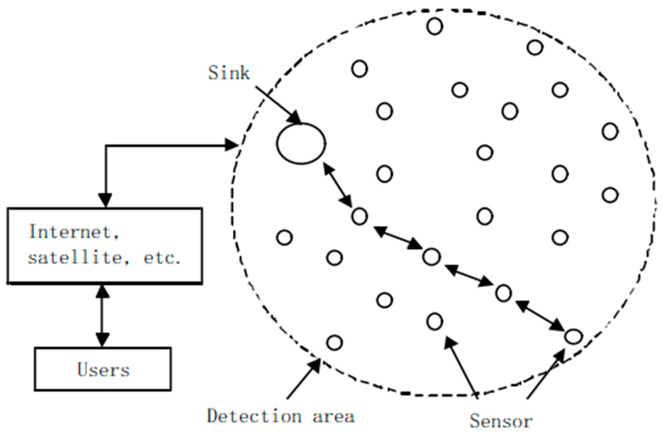
In order to improve the applicability of the evaluation algorithm (applicable to single-path transmission and multi-path transmission), this section considers converting the routing scheme into a single piece of data and performs real-time evaluation. When a node generates a routing scheme, routing scheme is converted into a single piece of data before transmitting data according to the scheme. To determine whether the data is abnormal is to evaluate in real time whether the routing scheme is feasible.
To improve evaluation accuracy and further reduce evaluation time, we employ machine learning algorithms to evaluate the routing scheme.
Unlabeled samples are more readily available than labeled samples. Since supervised learning requires all training data to be labeled, we chose semi-supervised learning with only a few labeled samples. Since there are only two types of labels, abnormal and non-anomalous, we chose a semi-supervised learning algorithm suitable for binary classification problems. Here, we chose the Semi-Supervised Support Vector Machine (S3VM). This type of algorithm has the following advantages: (1) There are less restrictions on the form of input data, which is conducive to reuse and training data generation. (2) The storage overhead is low, which is beneficial for us to process large-scale data. (3) It is simple and effective. Compared with other semi-supervised learning algorithms, the latency is relatively low, which can properly compensate for the timeliness shortcomings of evaluation methods.
The classic algorithm in the semi-supervised support vector machine is the Transduction Support Vector Machine (TSVM) [
11].
Assumption: Given a labeled sample set
and an unlabeled sample set
. (1 means abnormal, −1 means not abnormal),
.
The goal of TSVM is to predict the label of
(that is
) such that it satisfies Equation (1).
In Equation (1), is the relaxation vector; and are user-defined parameters for balancing the importance of labeled samples and unlabeled samples; determines a dividing hyperplane. TSVM continuously tries to assign labels to unlabeled samples, and the goal is to determine the partitioning hyperplane that maximizes the separation over all samples.
The flow of TSVM is shown in Algorithm 1. Algorithm 1 obtains the predicted labels for unlabeled samples and a final SVM model (hereinafter referred to as the TSVM model), which can be used to predict new samples.
| Algorithm 1: TSVM |
| 1: Input: labeled sample set , |
| 2: unlabeled sample set , |
| 3: parameters and |
| 4: Initialize and , ; |
| 5: Train an initial model SVM0 with ; |
| 6: Predict the label of with SVM0, obtain ; |
| 7: While |
| 8: Knowing , , , and , obtain and according to formula 1; |
| 9: While |
| 10: = −; |
| 11: = −; |
| 12: Knowing , , , and , obtain and according to formula 1; |
| 13: End while |
| 14: ; |
| 15: End while |
| 16: Output: , TSVM = SVMfinal |
We generate the initial multi-path routing scheme according to the wireless sensor network multi-path routing algorithm proposed in reference [
4]. The scheme includes p paths sorted according to the selection probability from large to small, and each path must have a node with the smallest remaining energy. The unlabeled samples in this paper contain the energy consumption and remaining energy of these p nodes.
Due to the different training data sets (including labeled samples and unlabeled samples) corresponding to different p and the high cost of manually obtaining training data, it is difficult for us to obtain enough training data for all possible p. To ensure efficient operation of TSVM and avoid overfitting, we need to ensure that there is enough training data. Therefore, we employ data augmentation to improve TSVM in an attempt to effectively augment the training data.
Supervised data augmentation is to expand more labeled data from the original labeled data through some transformation method, and then use the original data and augmented data to jointly train the model. The current general method is to fit the real sample distribution by adding sample points to continuous discrete sample points. We build on this idea for data augmentation in semi-supervised tasks.
We expand positive labeled samples, negative labeled samples and unlabeled samples, respectively. We leave the markup the same and expand in the same way. The expansion method is to insert a sample point
into the two discrete sample points
and
, and the calculation method of the interpolation is as shown in Equation (2).
In Equation (2), and are user-defined parameters, which are generally set to 0.5.
The flow of data enhancement for TSVM is shown in Algorithm 2.
| Algorithm 2: Data Enhancement for TSVM |
| 1: Read the training data set according to the number of paths p involved in the routing scheme; |
| 2: Input: labeled sample set , |
| 3: unlabeled sample set , |
| 4: parameters and |
| 5: Initialize and , ; |
| 6: // Expand labeled samples |
| 7: Train an initial model SVM0 with ; |
| 8: Split into and according to the positive or negative of y, and the number of samples are recorded as n+ and n− |
| 9: Perform high-dimensional clustering on the de-labeled sample sets of and ; |
| 10: FOR |
| 11: Randomly select a pair of samples from the largest cluster of ; |
| 12: Generate according to Equation (2); |
| 13: Predict the label of with SVM0, obtain ; |
| 14: IF |
| 15: Merge into ; |
| 16: END IF |
| 17: END FOR |
| 18: FOR |
| 19: Randomly select a pair of samples from the largest cluster of ; |
| 20: Generate according to Equation (2); |
| 21: Predict the label of with SVM0, obtain ; |
| 22: IF |
| 23: Merge into ; |
| 24: END IF |
| 25: END FOR |
| 26: // Expand unlabeled samples |
| 27: Train a model TSVM0 with , , , ; |
| 28: Perform high-dimensional clustering on ; |
| 29: FOR |
| 30: Randomly select a pair of samples from the largest cluster of ; |
| 31: Generate according to Equation (2); |
| 32: END FOR |
| 33: Train a model TSVM1 with , ; |
| 34: FOR |
| 35: Predict the label of with TSVM0 and TSVM1, obtain and ; |
| 36: IF |
| 37: Merge into ; |
| 38: END IF |
| 39: END FOR |
| 40: Output: Expanded and |
It is assumed that the routing scheme involves p paths in total, and each path has a minimum residual energy node, so the scheme includes p minimum residual energy nodes. The energy consumption of the i-th node is
, and the remaining energy is
. The scheme to be checked is
. The label y equal to 1 indicates that x is abnormal. The equation for determining the label is Equation (3). When the load ratio of a node exceeds a predetermined threshold (which may cause the node to fail) or the variance of the load of all nodes exceeds a predetermined threshold (indicating that the energy distribution is unreasonable, which may eventually lead to node failure), the logical value of Equation (3) is 1, that is, x is abnormal.
Combining Algorithms 1 and 2, we design and implement the real-time evaluation algorithm based on semi-supervised learning (RESL), whose flow is as in Algorithm 3.
| Algorithm 3: Real-time evaluation algorithm based on semi-supervised learning (RESL) |
1: Read the training data set according to the number of paths p involved in the
routing scheme; |
| 2: Input: labeled sample set , |
| 3: unlabeled sample set , |
| 4: the scheme to be checked |
| 5: IF |
| 6: Determine whether x is abnormal according to Equation (3), obtain y; |
| 7: ELSE |
| 8: IF |
| 9: Perform Algorithm 2; |
| 10: Perform Algorithm 1, obtain TSVM; |
| 11: Predict x with TSVM, obtain y; |
| 12: ELSE |
| 13: Perform Algorithm 1; |
| 14: Predict x with TSVM, obtain y; |
| 15: END IF |
| 16: END IF |
| 17: Output: y |
When the training data is not enough to train an effective model, use formula (3) to obtain the label; when the training data is enough to train the model but not enough to train a better model, the label is obtained after the data is enhanced; when the training data is enough to train a good model, the label is obtained directly.
2.2. Comparative Experiment
Taking time and accuracy as evaluation indicators, we compared the evaluation algorithm (RESL) proposed in this paper with the evaluation algorithm proposed in references [
9,
10]. The fuzzy evaluation algorithm (FEA) proposed in reference [
9] has a very low evaluation time, but the evaluation accuracy is not high; the adaptive evaluation algorithm (AEA) proposed in reference [
10] has a high evaluation accuracy, but the evaluation time is not low.
We measured and recorded the evaluation time and evaluation accuracy of the three algorithms for the same multi-path routing scheme.
We conducted a total of 500 trials and the results are shown in
Table 1. We used three algorithms to measure each of the 50 sets of data corresponding to p = 1~10 and recorded the evaluation accuracy.
If the path is selected more than twice (that is, the top two paths are not feasible), the actual result of the routing scheme is abnormal. We converted the routing plan to the corresponding data to be checked and used three evaluation algorithms to evaluate the data to be checked to obtain the judgment result (whether it is abnormal). If the judgment result is the same as the actual result, the evaluation is regarded as accurate. Since FEA and AEA both evaluate the multi-path routing scheme multiple times, if at least one abnormality occurs in the multiple evaluations, the judgment result is abnormal.
Plot
Table 1 as
Figure 2. It can be seen from
Figure 2 that the evaluation accuracy of RESL is much higher than that of FEA and slightly higher than that of AEA.
- 2.
Evaluation time
We conducted a total of 150 trials and the results are shown in
Table 2. We used three algorithms to measure each of the 50 sets of data corresponding to p = 1~10 and recorded the running time of the evaluation algorithm.
Since both FEA and AEA are single-path evaluations, they need to perform multiple evaluations for the multi-path solution, so their evaluation time counts the total time of multiple evaluations.
Plot
Table 2 as
Figure 3. It can be seen from
Figure 3 that the algorithm running time of RESL is lower than AEA but higher than FEA.
Although FEA has a great advantage in algorithm running time, its evaluation accuracy is not high. The time cost of evaluating errors introduced (rerouting time, etc.) is much higher than the running time of evaluating algorithms. Therefore, the overall evaluation time of using FEA in an evaluation-based routing algorithm is unstable and extremely time-consuming.
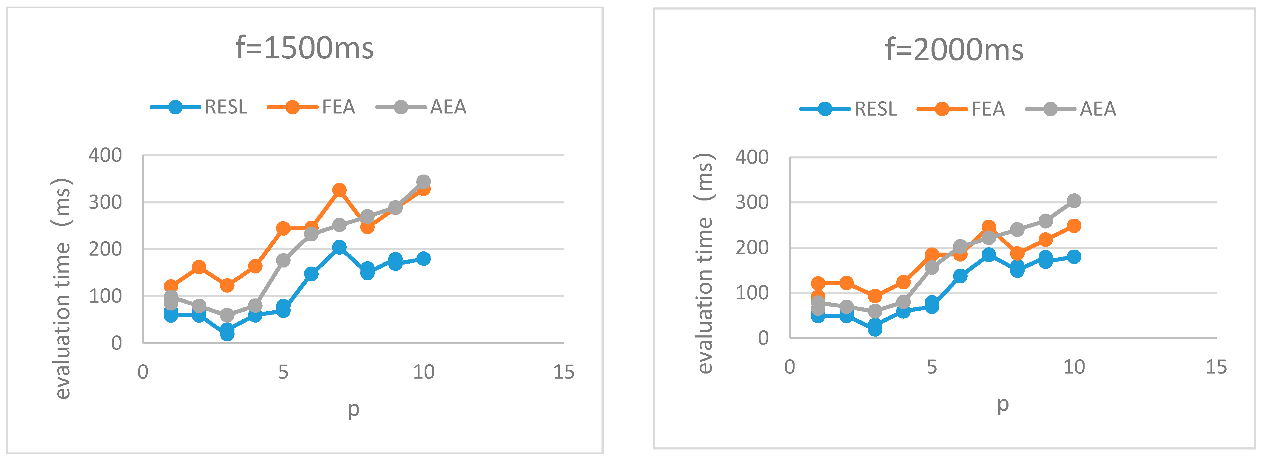
Assumption 1: Given that the running time of the algorithm is t, the evaluation accuracy is c and the time introduced by the evaluation error is f.
The evaluation time T for evaluating the routing scheme is defined as Equation (4).
Given different f, we combine
Table 1 and
Table 2 to obtain the evaluation time of the three algorithms, as shown in
Figure 4.
It can be seen from
Figure 4 that the evaluation time of RESL is lower than that of FEA and AEA.
In conclusion, RESL outperforms the two comparison algorithms in evaluation time and evaluation accuracy. (1) Compared with FEA with extremely low algorithm running time, the evaluation accuracy of RESL is much higher than that of FEA. Although the algorithm running time of RESL is higher than that of FEA, the evaluation time is lower than that of FEA. (2) Compared with AEA, which has a higher evaluation accuracy, the evaluation accuracy of RESL is slightly higher than that of AEA and the evaluation time is lower than that of AEA.


