
The Use of Drone Photo Material to Classify the Purity of Photovoltaic Panels Based on Statistical Classifiers

Abstract
:1. Introduction
- –
- Positive correlation between the intensity of sunlight and the daily demand for electricity,
- –
- Increased generation in the summer period correlated with the demand for cold, and
- –
- It enables the use of brownfield sites and poor-quality land, as well as building roofs [9].
- –
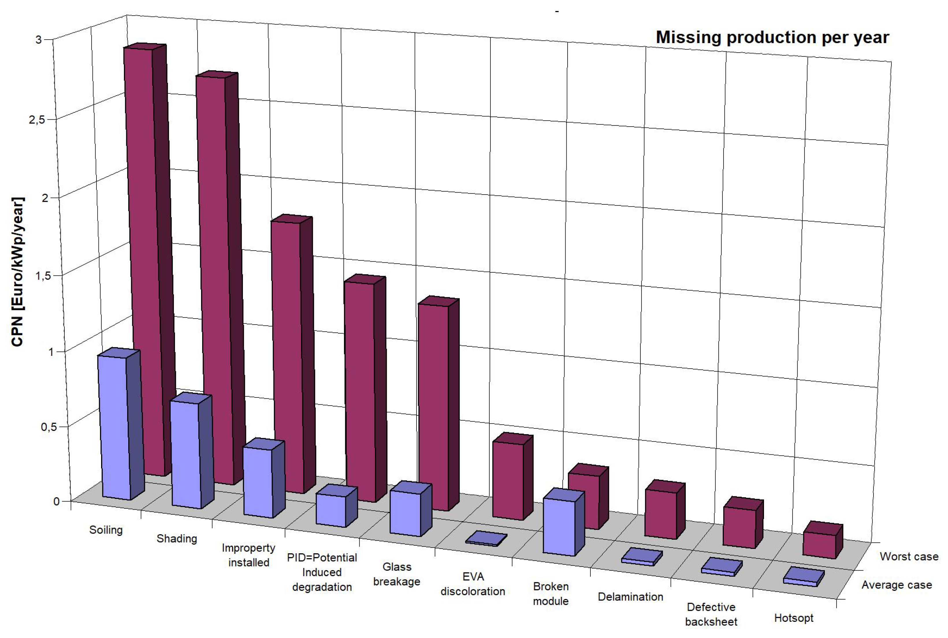
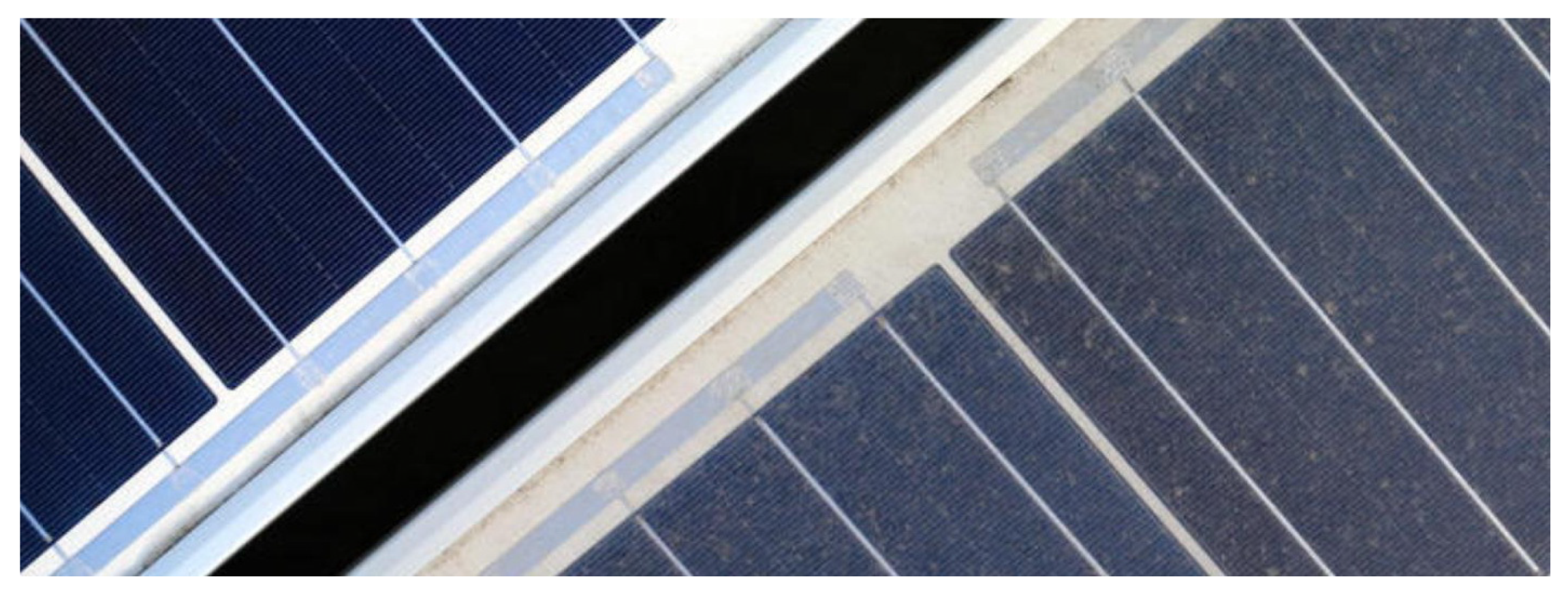
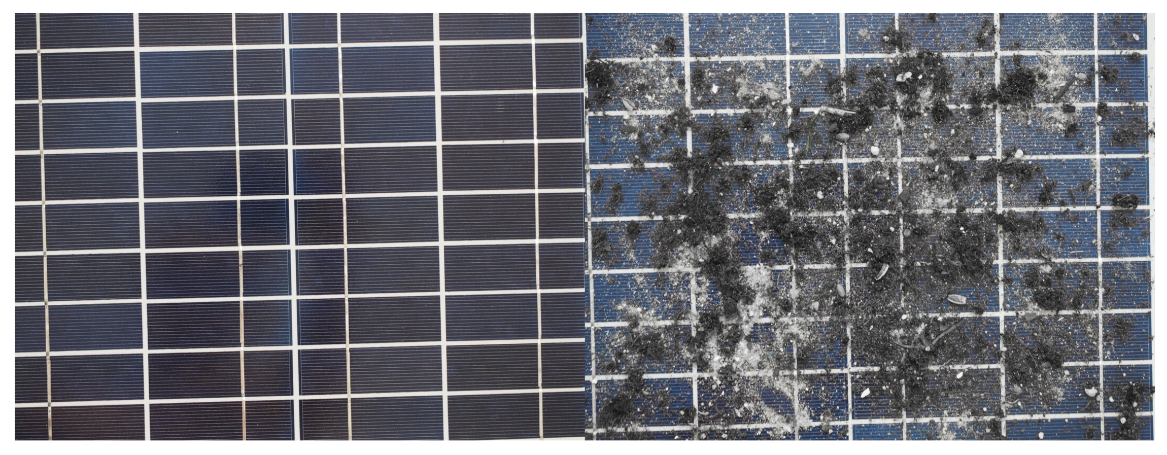
- Dirt on PV panels,
- –
- Incorrect installation,
- –
- Shading,
- –
- Discoloration of EVA foil,
- –
- Glass breakage,
- –
- Degradation by induced voltage,
- –
- Path snails,
- –
- Defective protective foil,
- –
- Spot heating of panels [10].
2. Requirements
- –
- Clean,
- –
- Dirty.
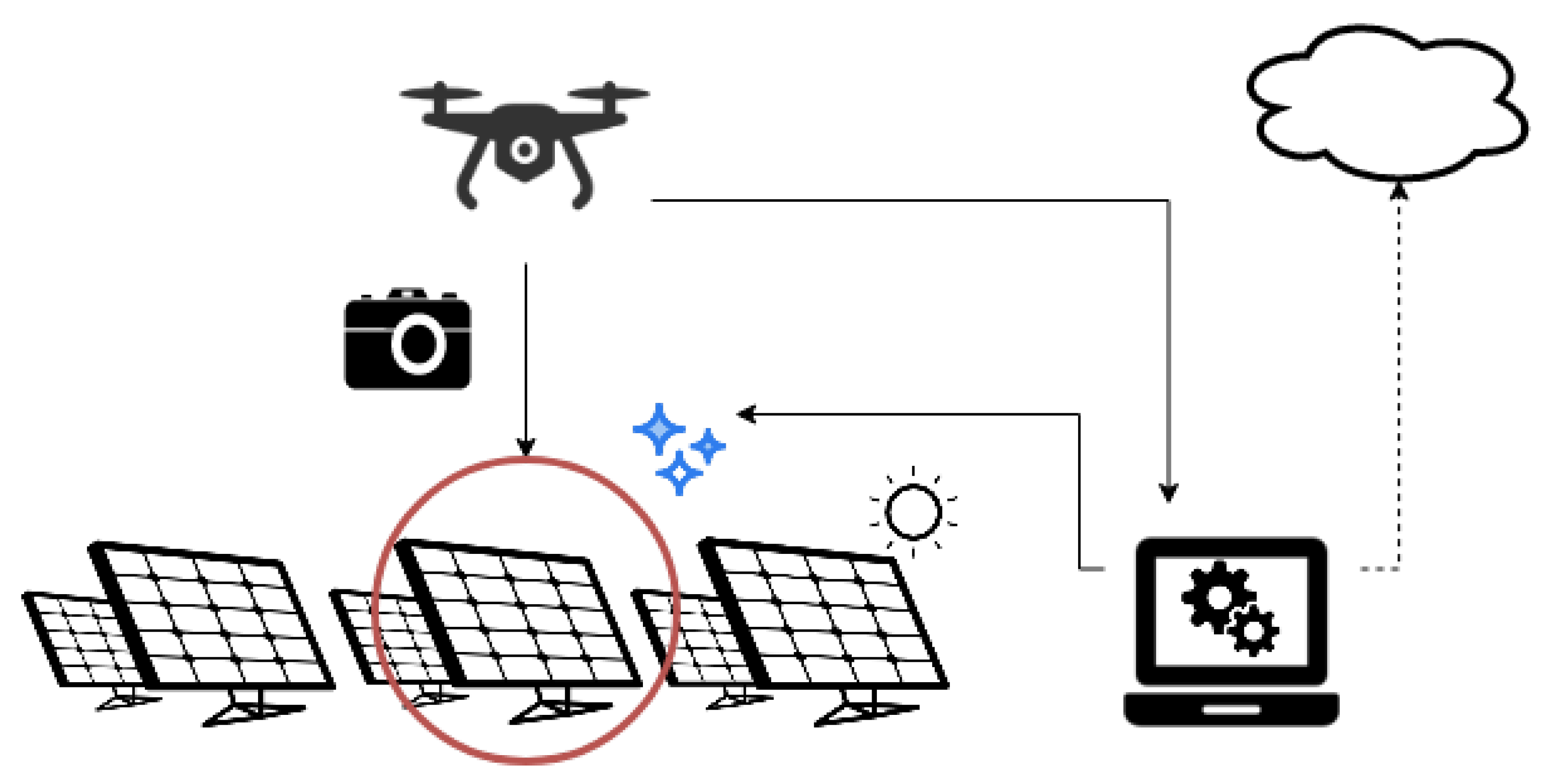
2.1. Drone Photo Sourcing
2.2. The Research Material
- –
- 60 photos containing one panel,
- –
- 4 photos containing two panels,
- –
- 4 photos containing three panels,
- –
- 2 photos contain four panels.
- –
- With adequate sunlight. The images were taken during the day with a minimum solar radiation intensity of 500 W/, because below this value the PV panels are insufficiently illuminated, which means that the contrast of the photo is too low to extract the information that is important to us. The project does not assume artificial lighting of PV panels.
- –
- Under appropriate weather conditions. Pictures cannot be taken during rainfall, as they introduce unwanted artifacts into the picture, making subsequent analysis difficult.
- –
- At a minimum angle of 45 to the panel surface. Smaller values may make it impossible to extract the panel from the photo.
- –
- At different times of the year. This approach will enable the use of classifiers throughout the year.
3. Statistical Classifiers to Classify Photovoltaic Panels
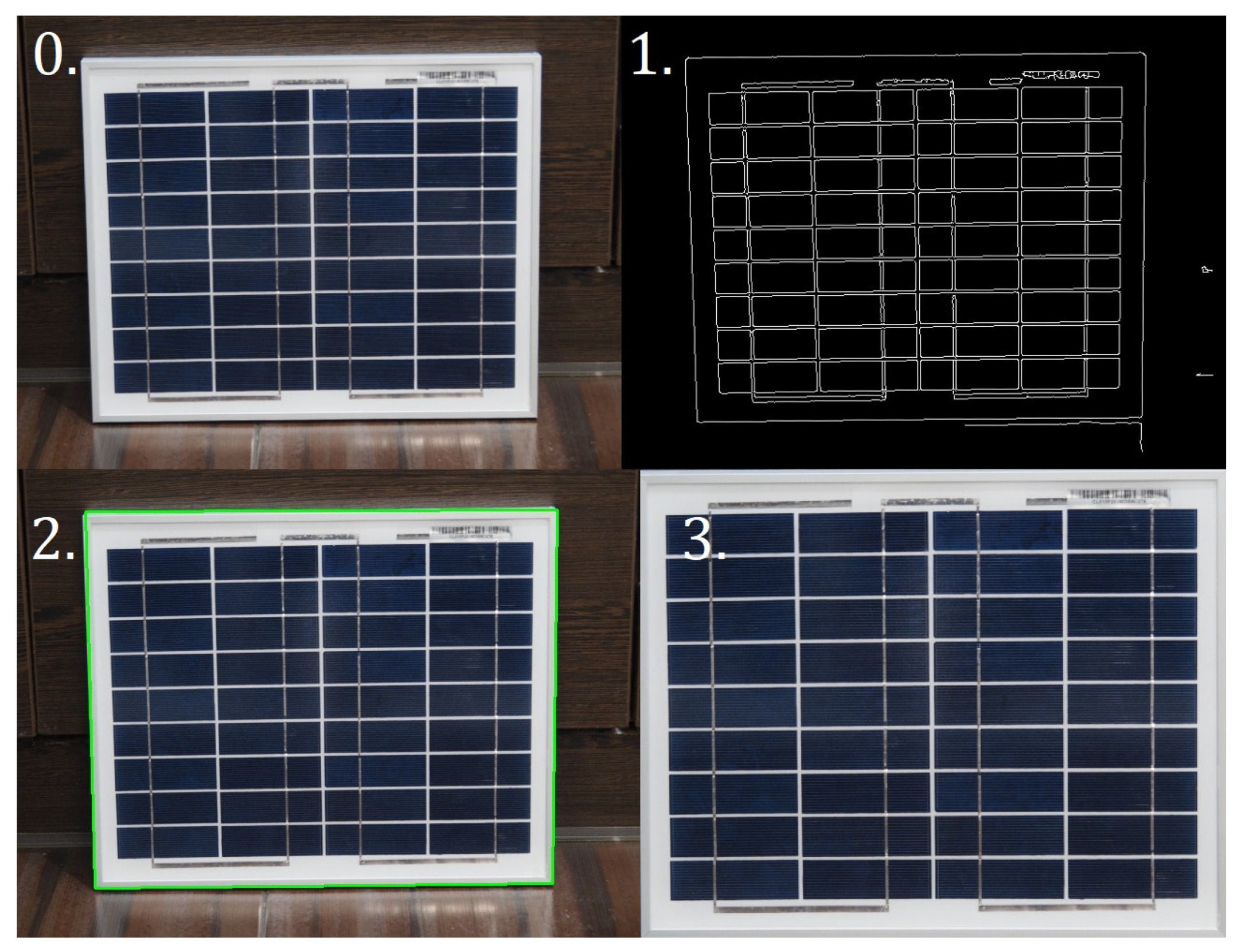
3.1. Extracting a Panel from a Photo
- –
- Detection of all edges in the photo,
- –
- Finding the edge of the PV panel,
- –
- Application of a forward-looking transformation [25].
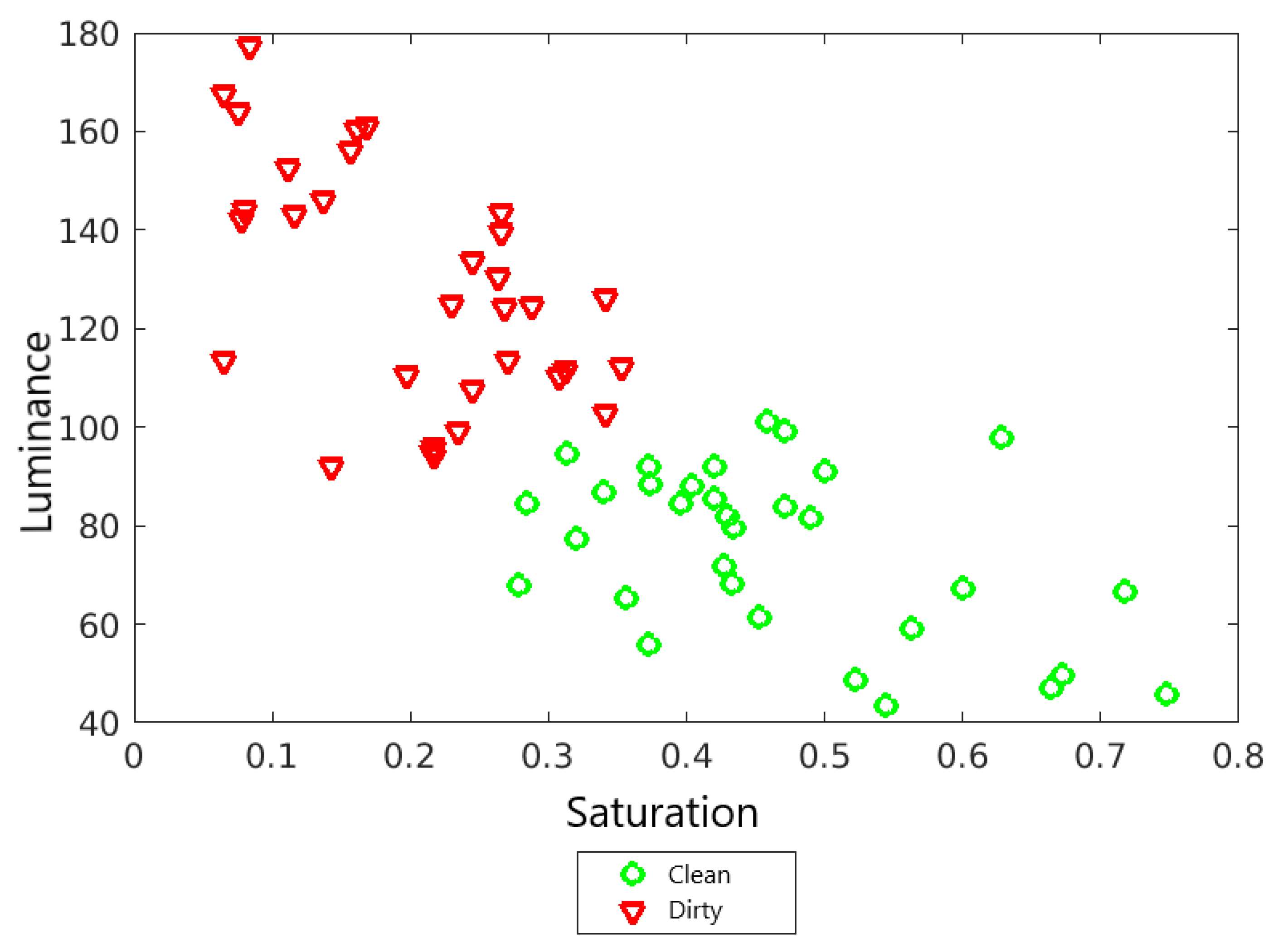
3.2. Observation
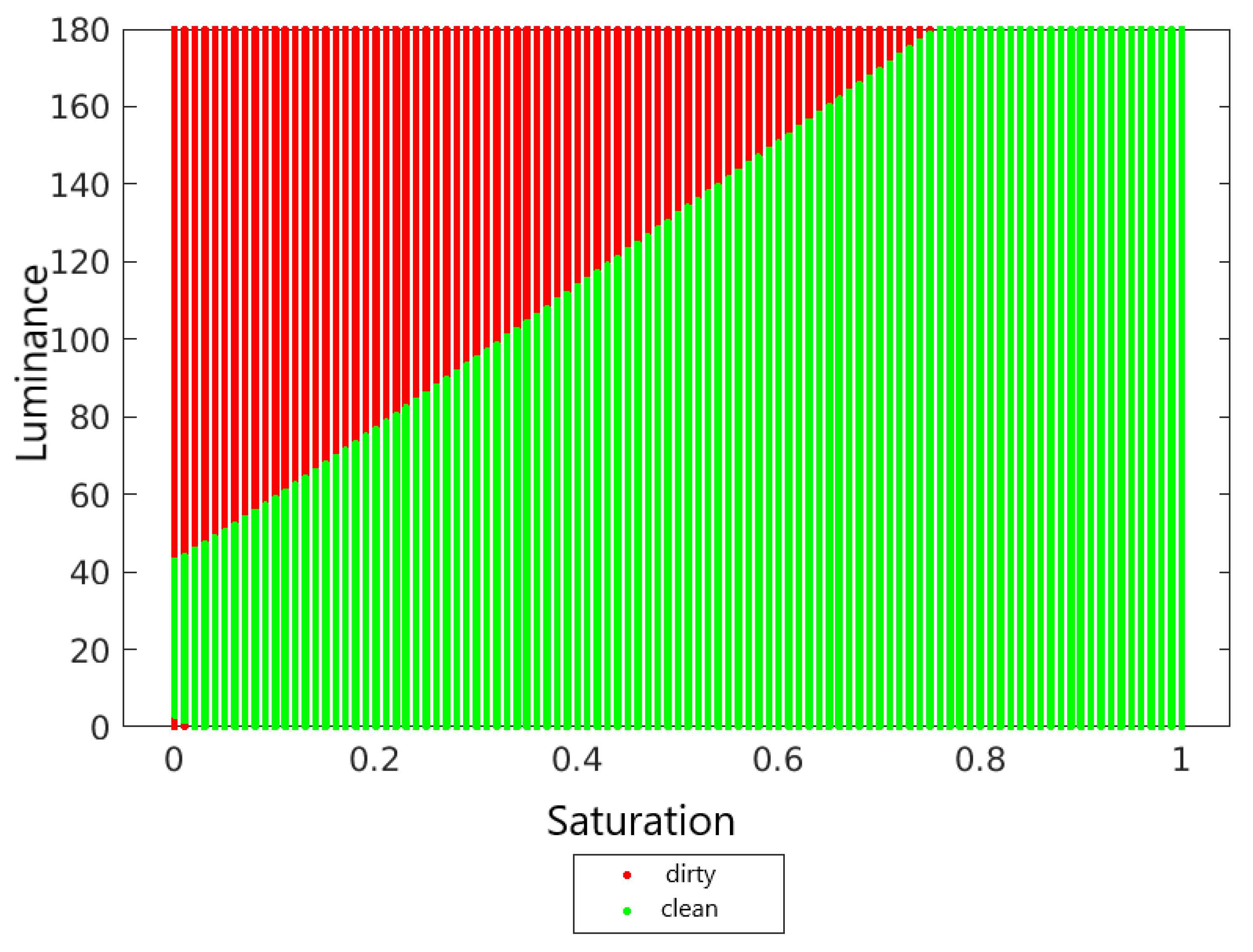
3.3. The Classifier of the k Nearest Neighbors
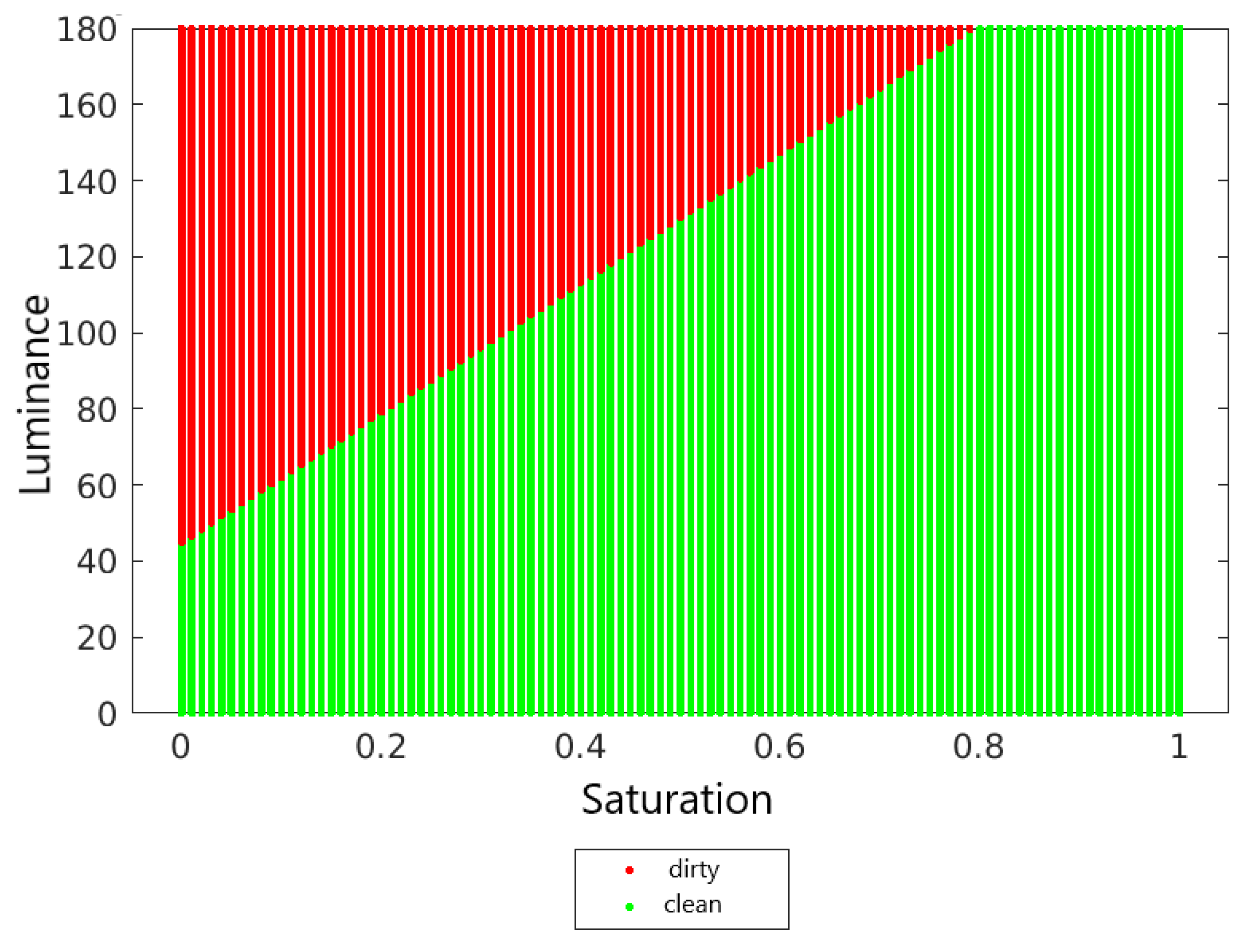
3.4. Naive Bayesian Classifier
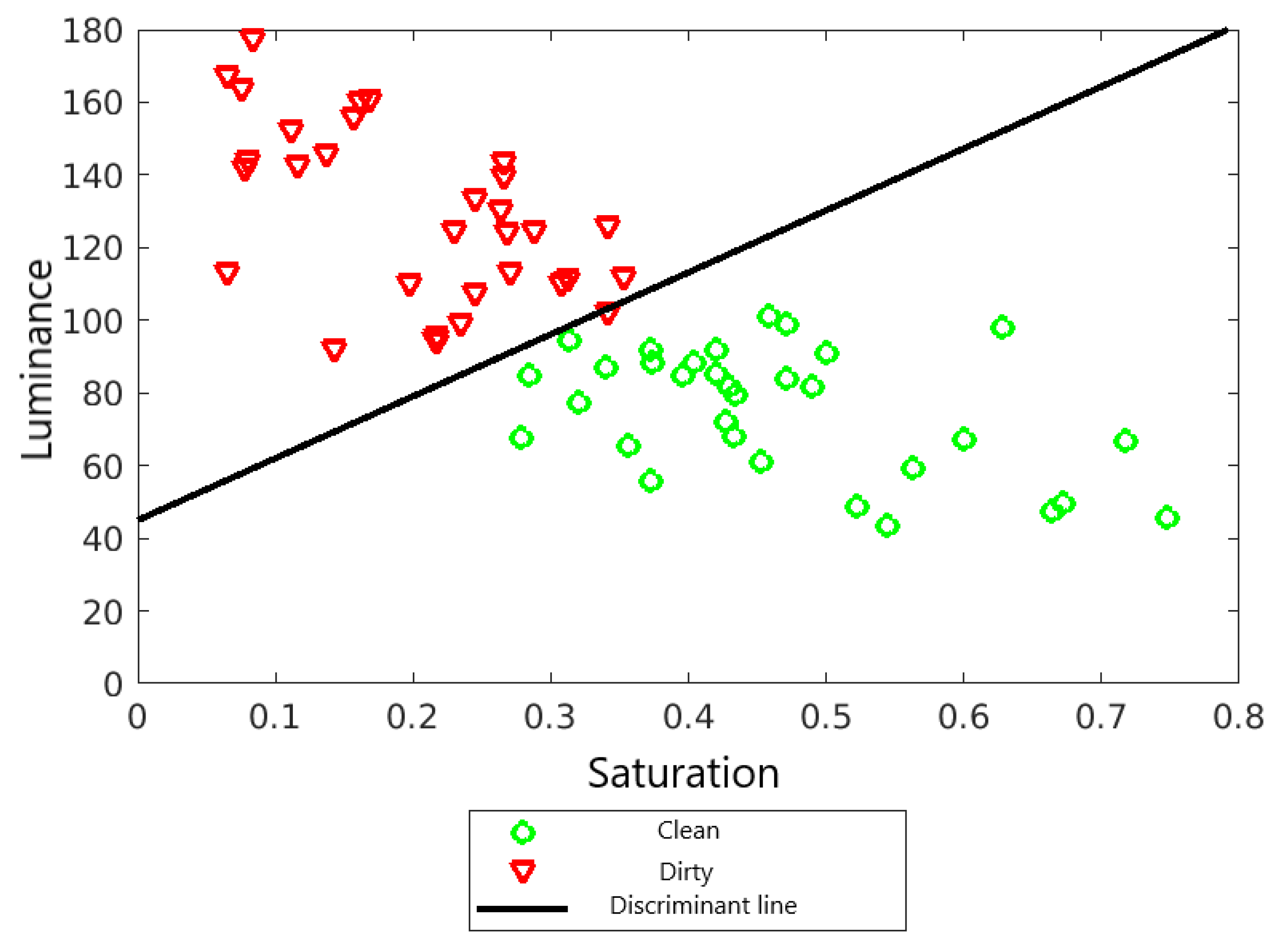
3.5. Fisher’s Linear Discriminator
find the direction a, hat best separates the learning subgroups, and as a measure of class separation along a given direction a take the square of the distance between the arithmetic means of the subgroups along this direction, taking into account the variability of the intra-group observation.
4. Analysis and Research
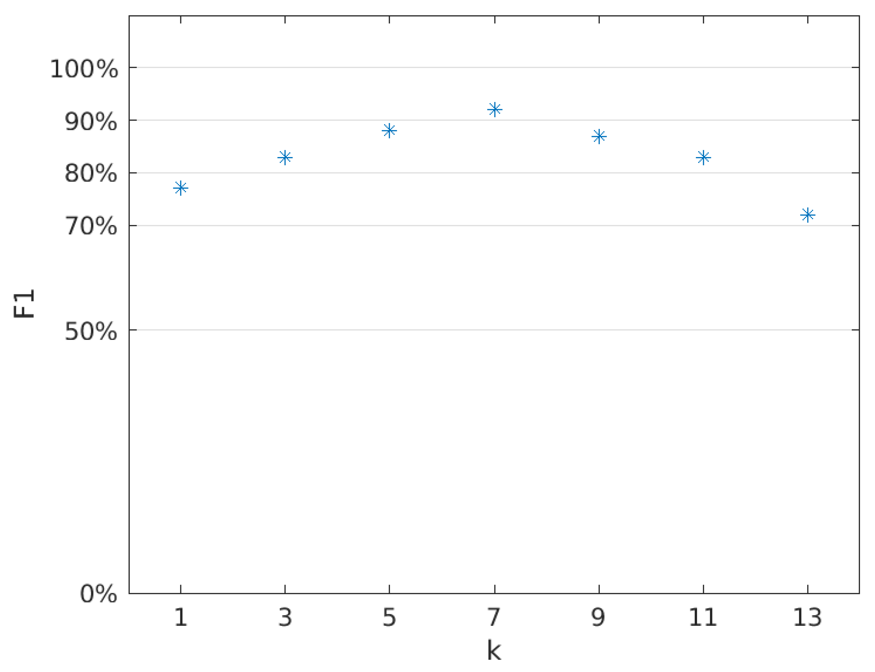
4.1. kNN Classifier
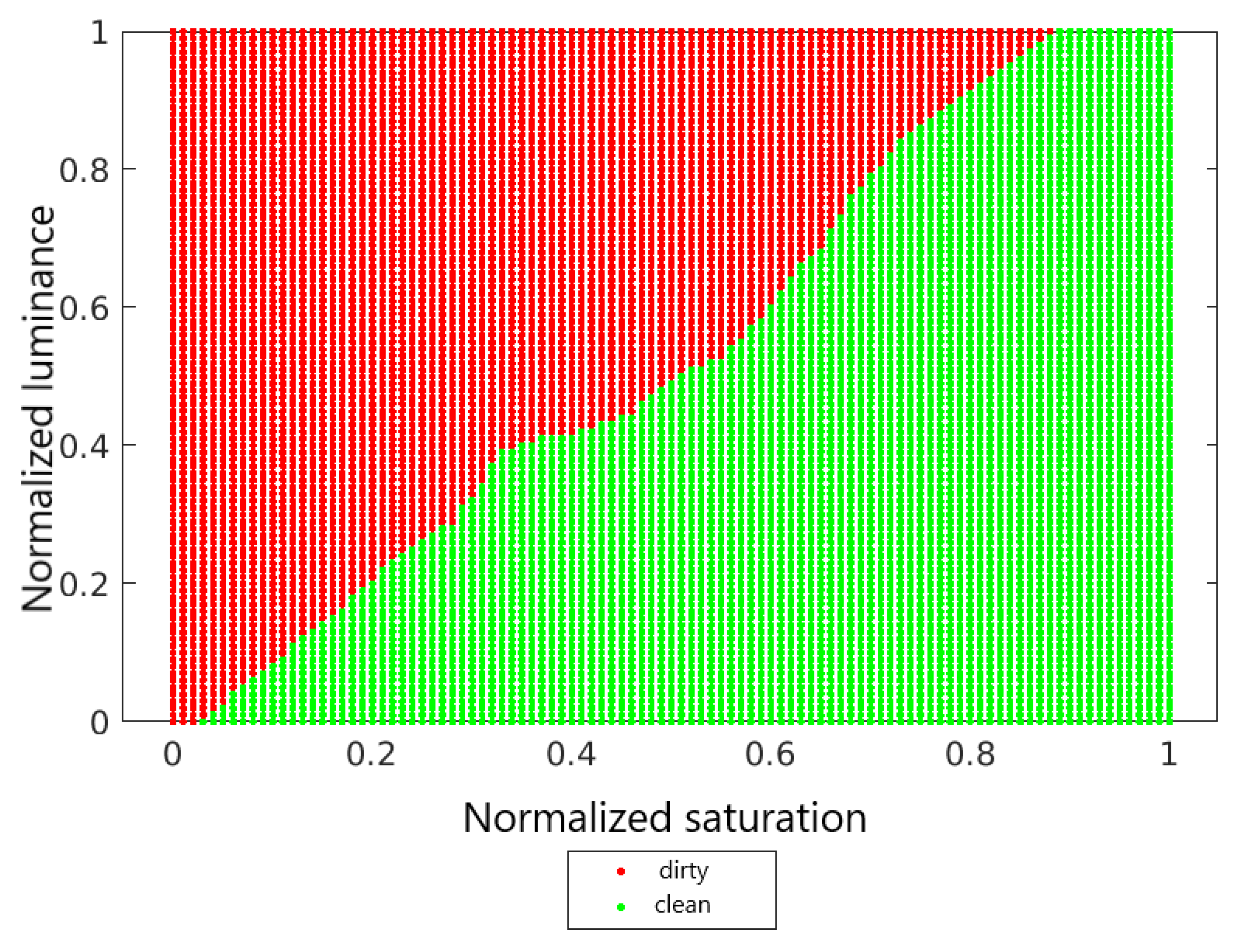
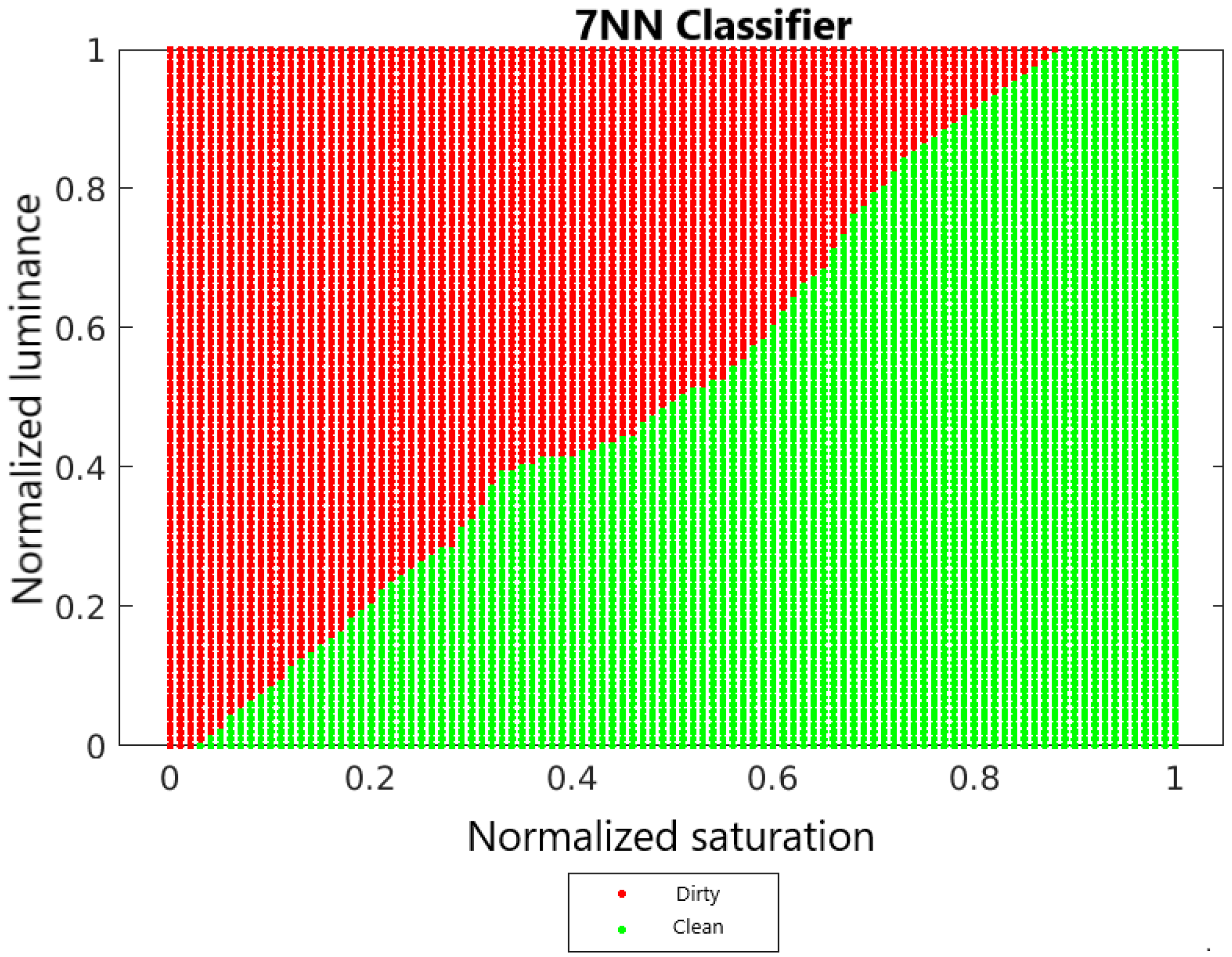
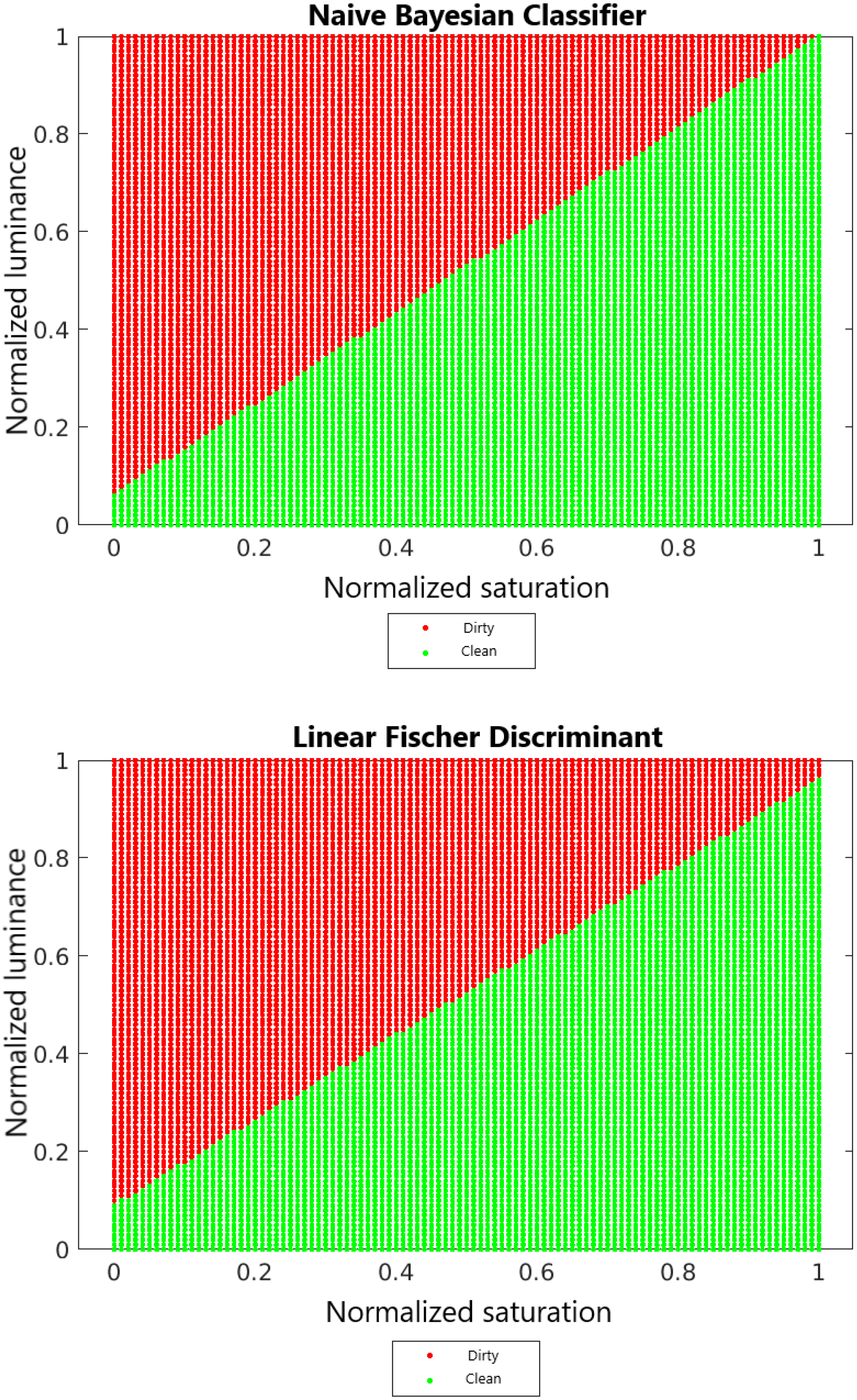
4.2. Decision Surfaces
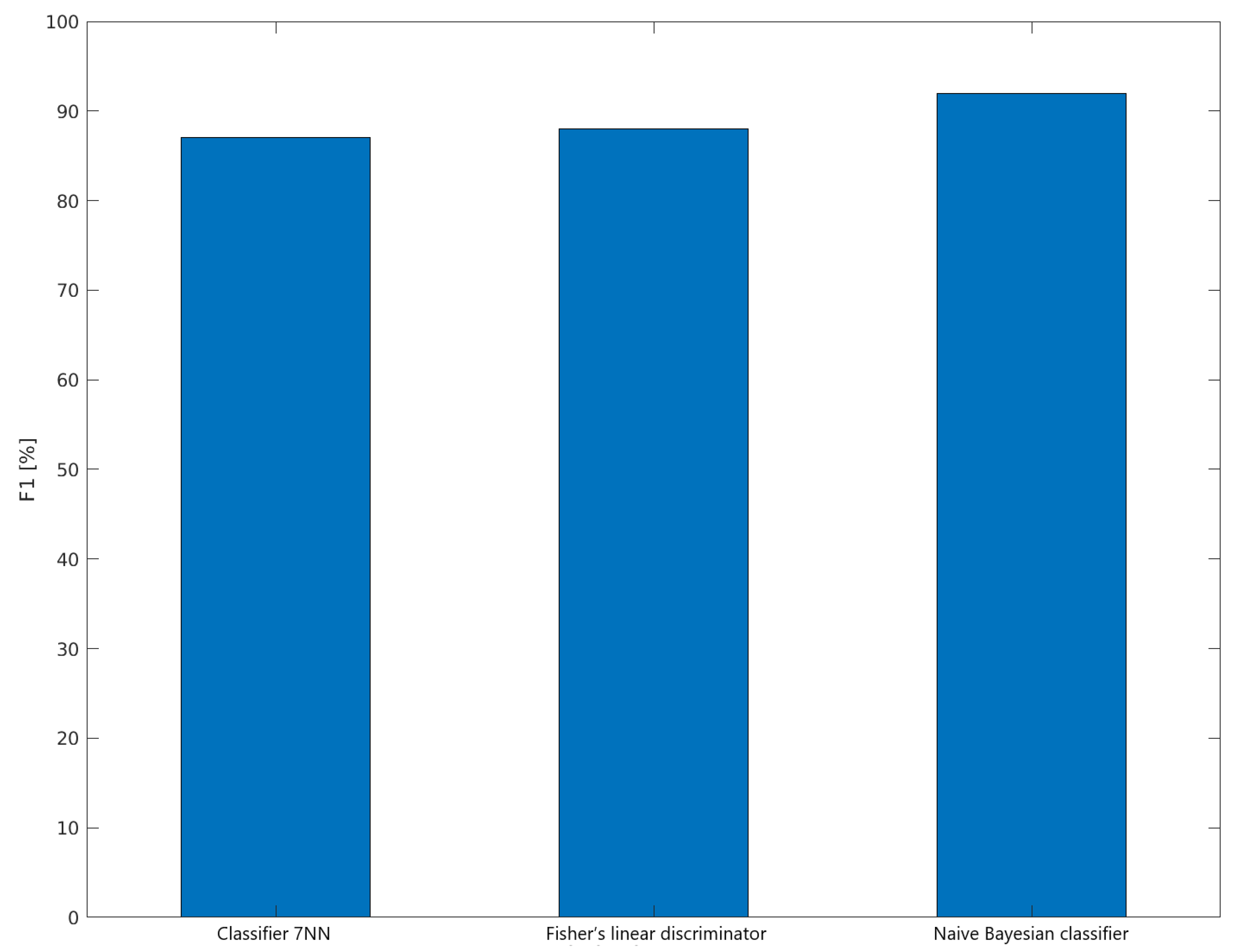
4.3. Metrics and Results
5. Summary
Author Contributions
Funding
Institutional Review Board Statement
Informed Consent Statement
Data Availability Statement
Conflicts of Interest
Abbreviations
| PV | photovoltaics |
| EVA | ethylene-vinyl acetate |
| TPR | true positive rate |
| TNR | true negative rate |
| PPV | positive predictive value |
| NPV | negative predictive value |
| P | positive |
| N | negative |
| TP | true positive |
| TN | true negative |
| FP | false positive |
| FN | false negative |
| RES | renewable energy sources |
| EU | European Union |
References
- GISTEMP Team. GISS Surface Temperature Analysis (GISTEMP), Version 4. NASA Goddard Institute for Space Studies. 2021. Available online: https://data.giss.nasa.gov/gistemp/ (accessed on 8 May 2012).
- Lenssen, N.; Schmidt, G.; Hansen, J.; Menne, M.; Persin, A.; Ruedy, R.; Zyss, D. Improvements in the GISTEMP uncertainty model. J. Geophys. Res. Atmos. 2019, 124, 6307–6326. [Google Scholar] [CrossRef]
- IPCC. Global Warming of 1.5 °C. An IPCC Special Report on the Impacts of Global Warming of 1.5 °C above Pre-Industrial Levels and Related Global Greenhouse Gas Emission Pathways, in the Context of Strengthening the Global Response to the Threat of Climate Change, Sustainable Development, and Efforts to Eradicate Poverty; Masson-Delmotte, V., Zhai, P., Pörtner, H.O., Roberts, D., Skea, J., Shukla, P.R., Pirani, A., Moufouma-Okia, W., Péan, C., Pidcock, R., Eds.; IPCC, 2019; In Press; Available online: https://www.ipcc.ch/site/assets/uploads/sites/2/2019/05/SR15_SPM_version_report_LR.pdf (accessed on 8 May 2012).
- Communication from the Commission to the European Parliament, the European Council, the Council, the European Economic and Social Committee and the Committee of the Regions the European Green Deal, Brussels. 11 December 2019, COM/2019/640 Final. Available online: https://www.eumonitor.eu/9353000/1/j4nvke1fm2yd1u0_j9vvik7m1c3gyxp/vl4cn7a3nez7/v=s7z/f=/com(2019)640_en.pdf (accessed on 8 May 2012).
- Proposal for a Regulation of the European Parliament and of the Council Establishing the Framework for Achieving Climate Neutrality and Amending REGULATION (EU) 2018/1999 (European Climate Law), Brussels, 4 March 2020. COM/2020/80 Final. Available online: https://ec.europa.eu/info/sites/default/files/commission-proposal-regulation-european-climate-lawmarch-2020_en.pdf (accessed on 8 May 2012).
- Amended Proposal for a Regulation of the European Parliament and of the Council on Establishing the Framework for Achieving Climate Neutrality and Amending REGULATION (EU) 2018/1999 (European Climate Law, Brussels, 17 September 2020. COM(2020) 563 Final, 2020/0036 (COD). Available online: https://eur-lex.europa.eu/legal-content/EN/TXT/PDF/?uri=CELEX:52020PC0563&rid=9 (accessed on 8 May 2012).
- What Is Green Power? Available online: https://19january2017snapshot.epa.gov/greenpower/what-green-power_.html (accessed on 8 May 2012).
- Moser, D.; Del Buono, M.; Jahn, U.; Herz, M.; Richter, M.; De Brabandere, K. Identification of technical risks in the photovoltaic value chain and quantification of the economic impact: Economic impact of technical risks in photovoltaic plants. Prog. Photovoltaics Res. Appl. 2017, 25, 592–604. [Google Scholar] [CrossRef]
- Ministry of National Assets. Poland’s National Energy and Climate Plan for the Years 2021–2030; Version 4.1; Ministry of National Assets, 2019. Available online: https://www.gov.pl/attachment/e64830c9-440f-4f17-b3e7-8abd7667d406 (accessed on 8 May 2012).
- David Moser, Giorgio Belluardo, Matteo Del Buono, Walter Bresciani, Elisa Veronese (EURAC) Ulrike Jahn, Magnus Herz, Eckart Janknecht, Erin Ndrio (TUV-RH) Karel de Brabandere, Mauricio Richter (3E); 1/3/2016. Available online: https://www.tuv.com/content-media-files/master-content/services/products/p06-solar/solar-downloadpage/solar-bankability_d1.1_d2.1_technical-risks-in-pv-projects.pdf (accessed on 8 May 2012).
- John, J.J.; Tatapudi, S.; Tamizhmani, G. Influence of soiling layer on quantum efficiency and spectral reflectance on crystalline silicon PV modules. In Proceedings of the 2014 IEEE 40th Photovoltaic Specialist Conference (PVSC), Denver, Co, USA, 8–13 June 2014; pp. 2595–2599. [Google Scholar] [CrossRef]
- Maghami, M.R.; Hizam, H.; Gomes, C.; Radzi, M.A.; Rezadad, M.I.; Hajighorbani, S. Power loss due to soiling on solar panel: A review. Renew. Sustain. Energy Rev. 2016, 59, 1307–1316. [Google Scholar] [CrossRef] [Green Version]
- Cai, S.; Bao, G.; Ma, X.; Wu, W.; Bian, G.B.; Rodrigues, J.J.; de Albuquerque, V.H.C. Parameters optimization of the dust absorbing structure for photovoltaic panel cleaning robot based on orthogonal experiment method. J. Clean. Prod. 2019, 217, 724–731. [Google Scholar] [CrossRef]
- Bessa, J.G.; Micheli, L.; Almonacid, F.; Fernández, E.F. Monitoring photovoltaic soiling: Assessment, challenges, and perspectives of current and potential strategies. Iscience 2021, 24, 102165. [Google Scholar] [CrossRef] [PubMed]
- Deb, D.; Brahmbhatt, N.L. Review of yield increase of solar panels through soiling prevention, and a proposed water-free automated cleaning solution. Renew. Sustain. Energy Rev. 2018, 82 Pt 3, 3306–3313. [Google Scholar] [CrossRef]
- Jiang, Y.; Lu, L.; Ferro, A.R.; Ahmadi, G. Analyzing wind cleaning process on the accumulated dust on solar photovoltaic (PV) modules on flat surfaces. Sol. Energy 2018, 159, 1031–1036. [Google Scholar] [CrossRef]
- Chanchangi, Y.N.; Ghosh, A.; Sundaram, S.; Mallick, T.K. An analytical indoor experimental study on the effect of soiling on PV, focusing on dust properties and PV surface material. Sol. Energy 2020, 203, 46–48. [Google Scholar] [CrossRef]
- Kim, D.; Youn, J.; Kim, C. Automatic Photovoltaic Panel Area Extraction from UAV Thermal Infrared Images. J. Korean Soc. Surv. Geod. Photogramm. Cartogr. 2016, 34, 559–568. [Google Scholar] [CrossRef] [Green Version]
- Ilse, K.; Micheli, L.; Figgis, B.W.; Lange, K.; Daßler, D.; Hanifi, H.; Wolfertstetter, F.; Naumann, V.; Hagendorf, C.; Gottschalg, R.; et al. Techno-Economic Assessment of Soiling Losses and Mitigation Strategies for Solar Power Generation. Joule 2019, 3, 2303–2321. [Google Scholar] [CrossRef] [Green Version]
- Sovetkin, E.; Steland, A. Automatic processing and solar cell detection in photovoltaic electroluminescence images. Integr. Comput.-Aided Eng. 2018, 26, 1–15. [Google Scholar] [CrossRef] [Green Version]
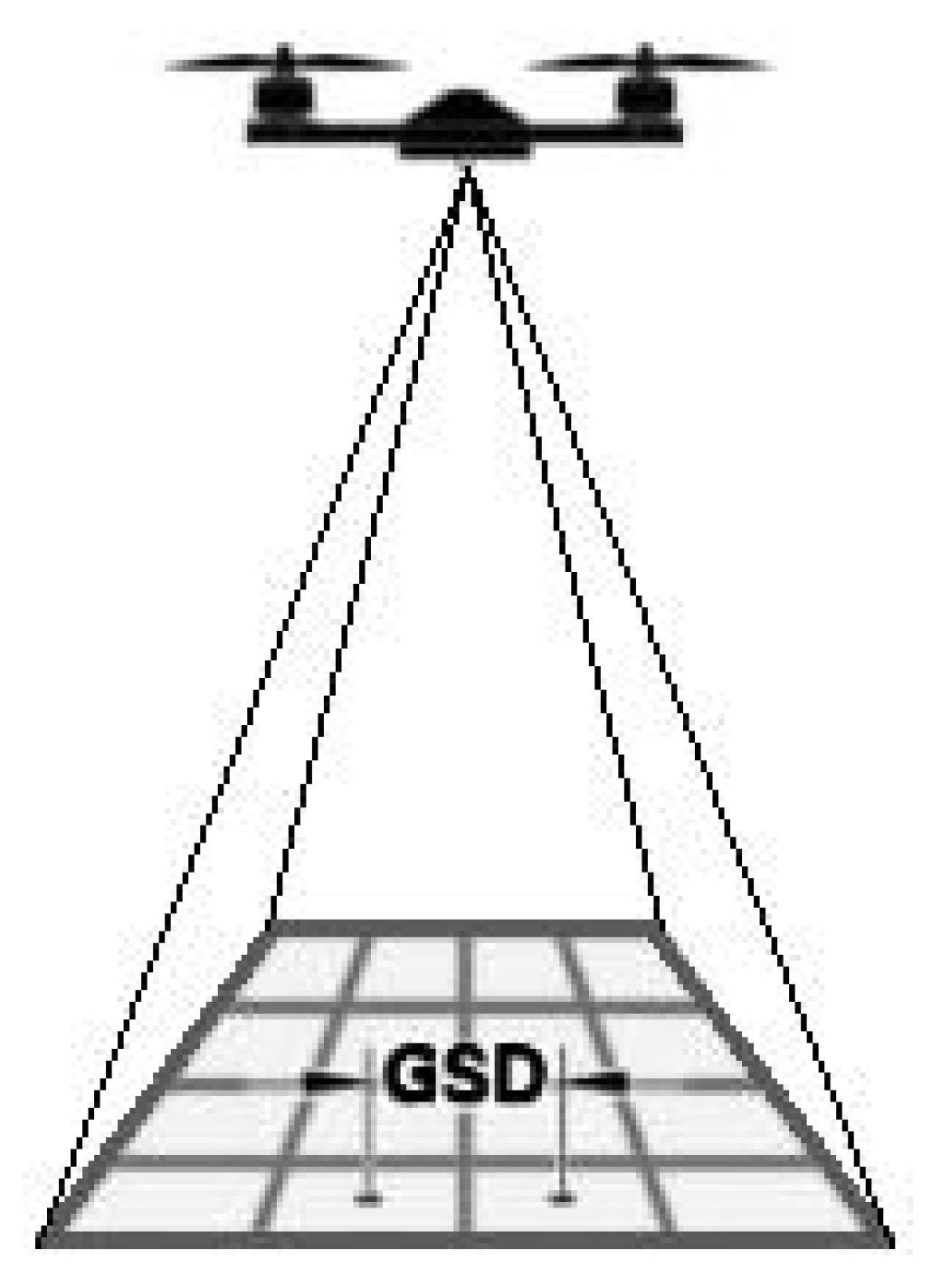
- Felipe-García, B.; Hernández-López, D.; Lerma, J.L. Analysis of the ground sample distance on large photogrammetric surveys. Appl. Geomat. 2012, 4, 231–244. [Google Scholar] [CrossRef]
- Seifert, E.; Seifert, S.; Vogt, H.; Drew, D.; Van Aardt, J.; Kunneke, A.; Seifert, T. Influence of Drone Altitude, Image Overlap, and Optical Sensor Resolution on Multi-View Reconstruction of Forest Images. Remote Sens. 2019, 11, 1252. [Google Scholar] [CrossRef] [Green Version]
- Jiang, H.; Yao, L.; Lu, N.; Qin, J.; Liu, T.; Liu, Y.; Zhou, C. Multi-resolution dataset for photovoltaic panel segmentation from satellite and aerial imagery. Earth Syst. Sci. Data 2021, 13, 5389–5401. [Google Scholar] [CrossRef]
- Hwang, Y.S.; Schlüter, S.; Park, S.I.; Um, J.S. Comparative Evaluation of Mapping Accuracy between UAV Video versus Photo Mosaic for the Scattered Urban Photovoltaic Panel. Remote Sens. 2021, 13, 2745. [Google Scholar] [CrossRef]
- Dharampal, V.M. Methods of Image Edge Detection: A Review. J. Electr. Electron. Syst. 2015, 4, 2. [Google Scholar] [CrossRef] [Green Version]
- Cao, D.H.; Stoumpos, C.C.; Farha, O.K.; Hupp, J.T.; Kanatzidis, M.G. 2D Homologous Perovskites as Light-Absorbing Materials for Solar Cell Applications. J. Am. Chem. Soc. 2015, 137, 7843–7850. [Google Scholar] [CrossRef] [PubMed]
- BT.601: Studio Encoding Parameters of Digital Television for Standard 4:3 and Wide Screen 16:9 Aspect Ratios. Available online: https://www.itu.int/rec/R-REC-BT.601 (accessed on 12 October 2021).
- Cheko, B. Introduction to Scene Text and Object Detection and Recognition Understanding A Scene Image; Scholars’ Press: Chisinau, Moldova, 2020; ISSN 978-613-8-93317-5. [Google Scholar]
- Cunningham, P.; Delany, S. k-Nearest neighbour classifiers. Mult. Classif. Syst. 2007, 54. [Google Scholar] [CrossRef]
- Bayindir, R.; Yesilbudak, M.; Colak, M.; Genc, N. A Novel Application of Naive Bayes Classifier in Photovoltaic Energy Prediction. In Proceedings of the 2017 16th IEEE International Conference on Machine Learning and Applications (ICMLA), Cancun, Mexico, 18–21 December 2017; pp. 523–527. [Google Scholar] [CrossRef]
- Mello, R.F. Moacir Antonelli Ponti, Machine Learning: A Practical Approach on the Statistical Learning Theory, 1st ed; Springer: Berlin/Heidelberg, Germany, 2018; ISBN 978-3319949888. [Google Scholar]
- Kohl, M. Performance Measures in Binary Classification. Int. J. Stat. Med. Res. 2012, 1, 79–81. [Google Scholar] [CrossRef]
- Canbek, G.; Temizel, T.T.; Sagiroglu, S.; Baykal, N. Binary Classification Performance Measures/Metrics: A Comprehensive Visualized Roadmap to Gain New Insights. In Proceedings of the 2017 International Conference on Computer Science and Engineering (UBMK), Antalya, Turkey, 5–8 October 2017; pp. 821–826. [Google Scholar] [CrossRef]
- Haeberlin, H.; Schaerf, P. Long-term Behaviour of Grid-Connected PV Systems over more than 15 Years. In Proceedings of the 5th European Photovoltaic Solar Energy Conference/5th World Conference on Photovoltaic Energy Conversion, Valencia, Spain, 6–10 September 2010; Available online: http://www.pvtest.ch/Dokumente/Publikationen/144_LZPV4-Valencia-K_F_02.pdf (accessed on 8 May 2012).


| Clean | Dirty | |
|---|---|---|
| Saturation | 0.4707 | 0.0891 |
| Luminance | 84.3143 | 143.0543 |
| k | P | N | TP | TN | FP | FN |
|---|---|---|---|---|---|---|
| 1 | 12 | 12 | 10 | 8 | 4 | 2 |
| 3 | 12 | 12 | 10 | 10 | 2 | 2 |
| 5 | 12 | 12 | 11 | 10 | 2 | 1 |
| 7 | 12 | 12 | 11 | 11 | 1 | 1 |
| 9 | 12 | 12 | 10 | 11 | 1 | 2 |
| 11 | 12 | 12 | 10 | 10 | 2 | 2 |
| 13 | 12 | 12 | 9 | 8 | 3 | 2 |
| k | TPR | TNR | PPV | NPV | F1 |
|---|---|---|---|---|---|
| 1 | 83% | 67% | 71% | 80% | 77% |
| 3 | 83% | 83% | 83% | 83% | 83% |
| 5 | 92% | 83% | 85% | 91% | 88% |
| 7 | 92% | 92% | 92% | 92% | 92% |
| 9 | 83% | 92% | 91% | 85% | 87% |
| 11 | 83% | 83% | 83% | 83% | 83% |
| 13 | 75% | 67% | 69% | 73% | 72% |
| Classifier | P | N | TP | TN | FP | FN |
|---|---|---|---|---|---|---|
| The classifier of the k nearest neighbors | 12 | 12 | 10 | 11 | 1 | 2 |
| Naive Bayesian classifier | 12 | 12 | 11 | 11 | 1 | 1 |
| Fisher’s linear discriminator | 12 | 12 | 11 | 10 | 2 | 1 |
| Classifier | TPR | TNR | PPV | NPV | F1 |
|---|---|---|---|---|---|
| Classifier 7NN | 83% | 92% | 91% | 85% | 87% |
| Naive Bayesian classifier | 92% | 92% | 92% | 92% | 92% |
| Fisher’s linear discriminator | 92% | 83% | 85% | 91% | 88% |
Publisher’s Note: MDPI stays neutral with regard to jurisdictional claims in published maps and institutional affiliations. |
© 2022 by the authors. Licensee MDPI, Basel, Switzerland. This article is an open access article distributed under the terms and conditions of the Creative Commons Attribution (CC BY) license (https://creativecommons.org/licenses/by/4.0/).
Share and Cite
Czarnecki, T.; Bloch, K. The Use of Drone Photo Material to Classify the Purity of Photovoltaic Panels Based on Statistical Classifiers. Sensors 2022, 22, 483. https://doi.org/10.3390/s22020483
Czarnecki T, Bloch K. The Use of Drone Photo Material to Classify the Purity of Photovoltaic Panels Based on Statistical Classifiers. Sensors. 2022; 22(2):483. https://doi.org/10.3390/s22020483
Chicago/Turabian StyleCzarnecki, Tomasz, and Kacper Bloch. 2022. "The Use of Drone Photo Material to Classify the Purity of Photovoltaic Panels Based on Statistical Classifiers" Sensors 22, no. 2: 483. https://doi.org/10.3390/s22020483
APA StyleCzarnecki, T., & Bloch, K. (2022). The Use of Drone Photo Material to Classify the Purity of Photovoltaic Panels Based on Statistical Classifiers. Sensors, 22(2), 483. https://doi.org/10.3390/s22020483