


Deep Learning-Based Synthesized View Quality Enhancement with DIBR Distortion Mask Prediction Using Synthetic Images


Abstract
1. Introduction
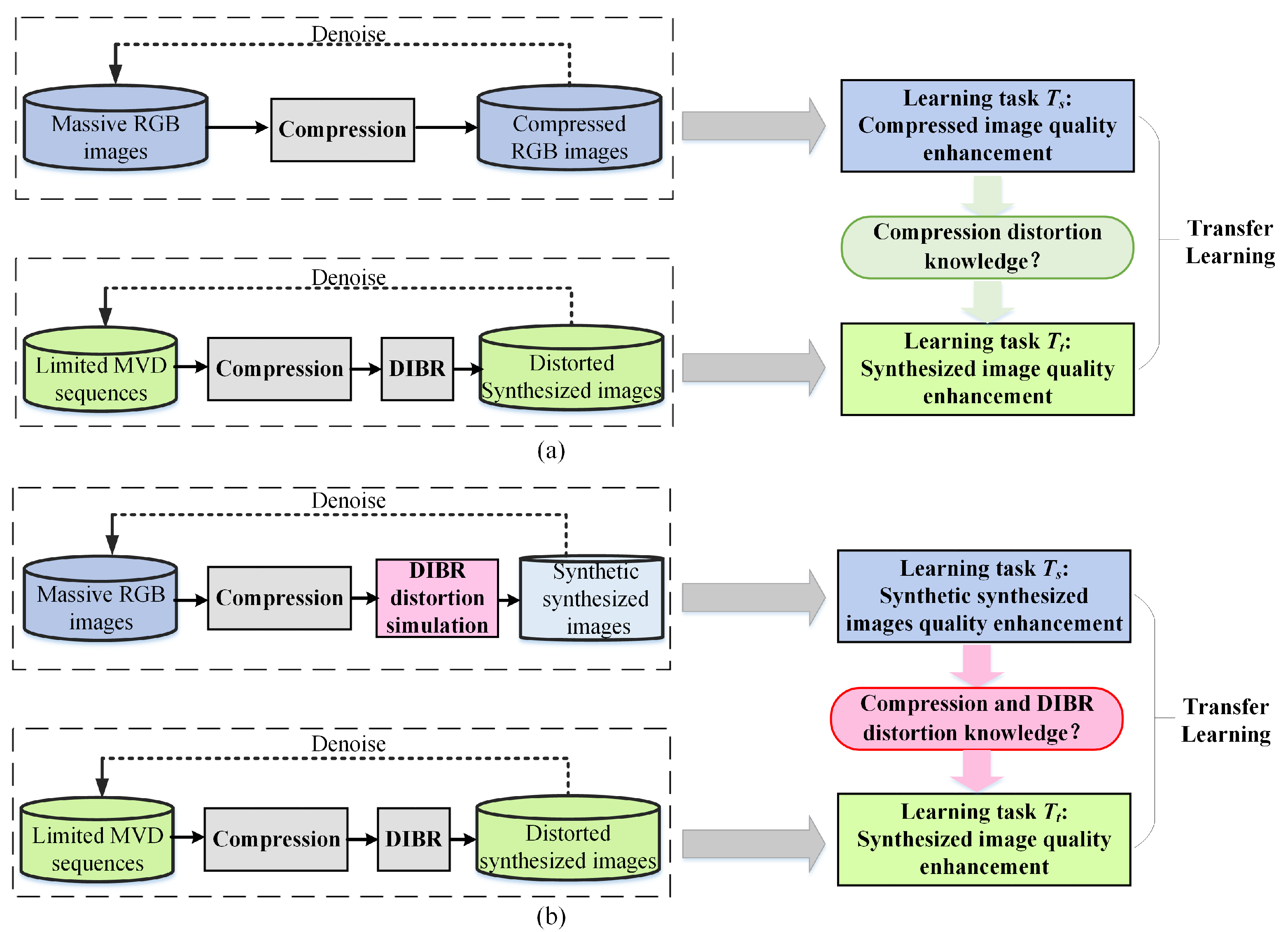
- A transfer learning-based scheme for the SVQE task is proposed, in which the SVQE model is first pre-trained on a synthetic synthesized view database, then fine-tuned on the MVD database;
- A synthetic synthesized view database is constructed in which a specific data synthesis method based on the random irregular polygon generation method simulating the special characteristics of SVI distortion is proposed, which has been validated on well-known state-of-the-art denoising or SVQE models on public RGB/RGBD databases;
- A sub-network is employed to predict the DIBR distortion mask and embedded with SVQE models using synthetic SVIs. The attempt of explicitly introducing the DIBR distortion position information is proved to be effective in elevating the performance of SVQE models.
2. Related Work
2.1. SVQE Models

| Methods | Hand-Crafted | CNN-Based | Transformer-Based | General 2D Images | Synthesized Views | Main Noise Types |
|---|---|---|---|---|---|---|
| NLM [7], BM3D [8] | ✔ | ✔ | Gaussian noise | |||
| DnCNN [2], FFDNet [9], CBDNet [3], RDN [4], NAFNet [10] | ✔ | ✔ | Gaussian noise, blur, real image noise, low resolution | |||
| Restormer [11], SwinIR [12] | ✔ | ✔ | ||||
| VRCNN [13], Zhu et al. [16], TSAN [5], RDEN [6], SynVD-Net [1] | ✔ | ✔ | Compression distortion, DIBR distortion |
2.2. Image Data Augmentation and Data Synthesis
2.3. Distortion Mask Prediction
3. Method
3.1. Motivation
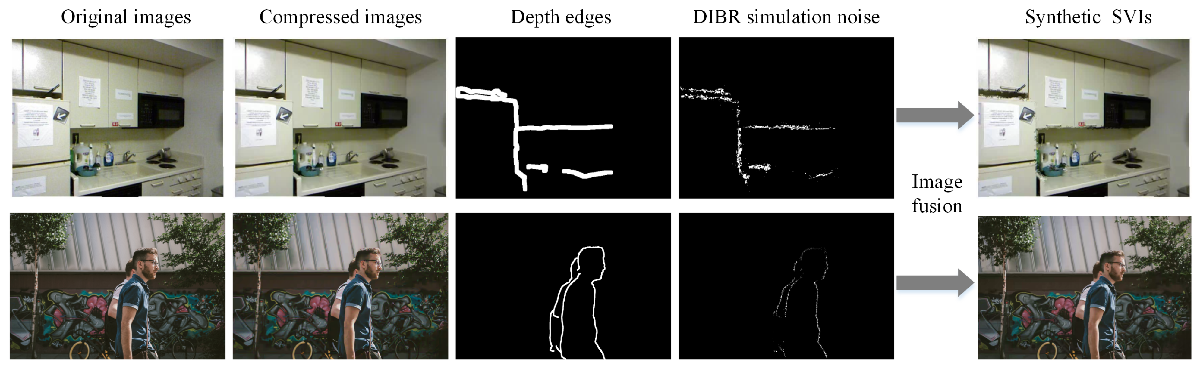
3.2. DIBR Distortion Simulation
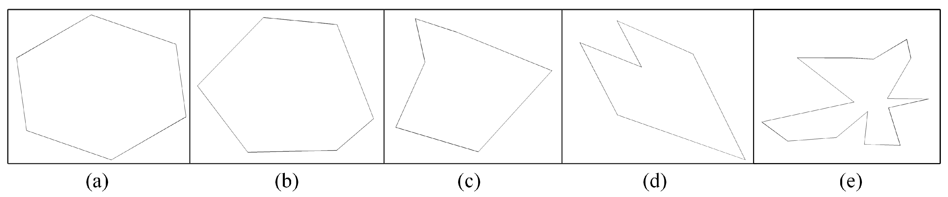
3.3. Different Local Noise Comparison and Proposed Random Irregular Polygon-Based DIBR Distortion Generation
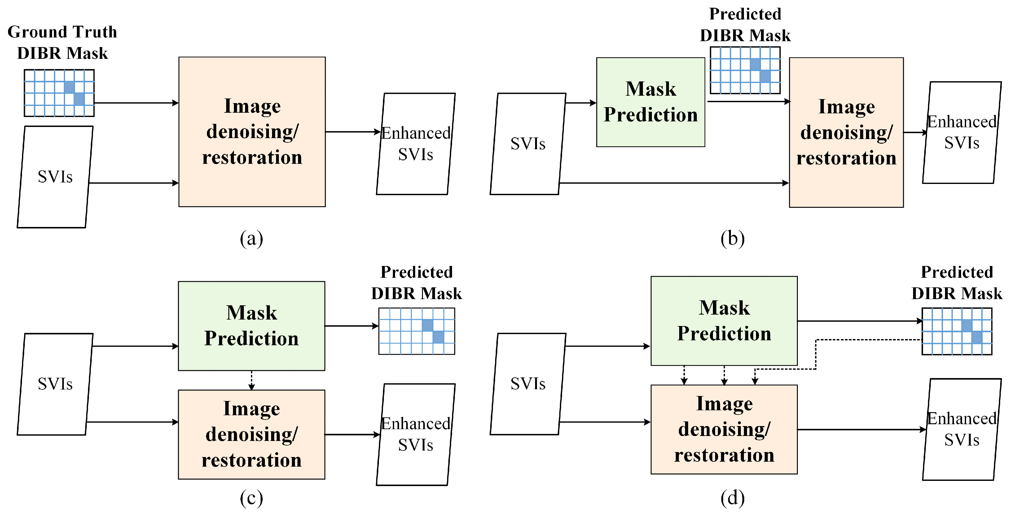
3.4. DIBR Distortion Mask Prediction Network Embedding
4. Datasets Preparation
5. Experimental Results and Analysis
5.1. Experimental Configuration
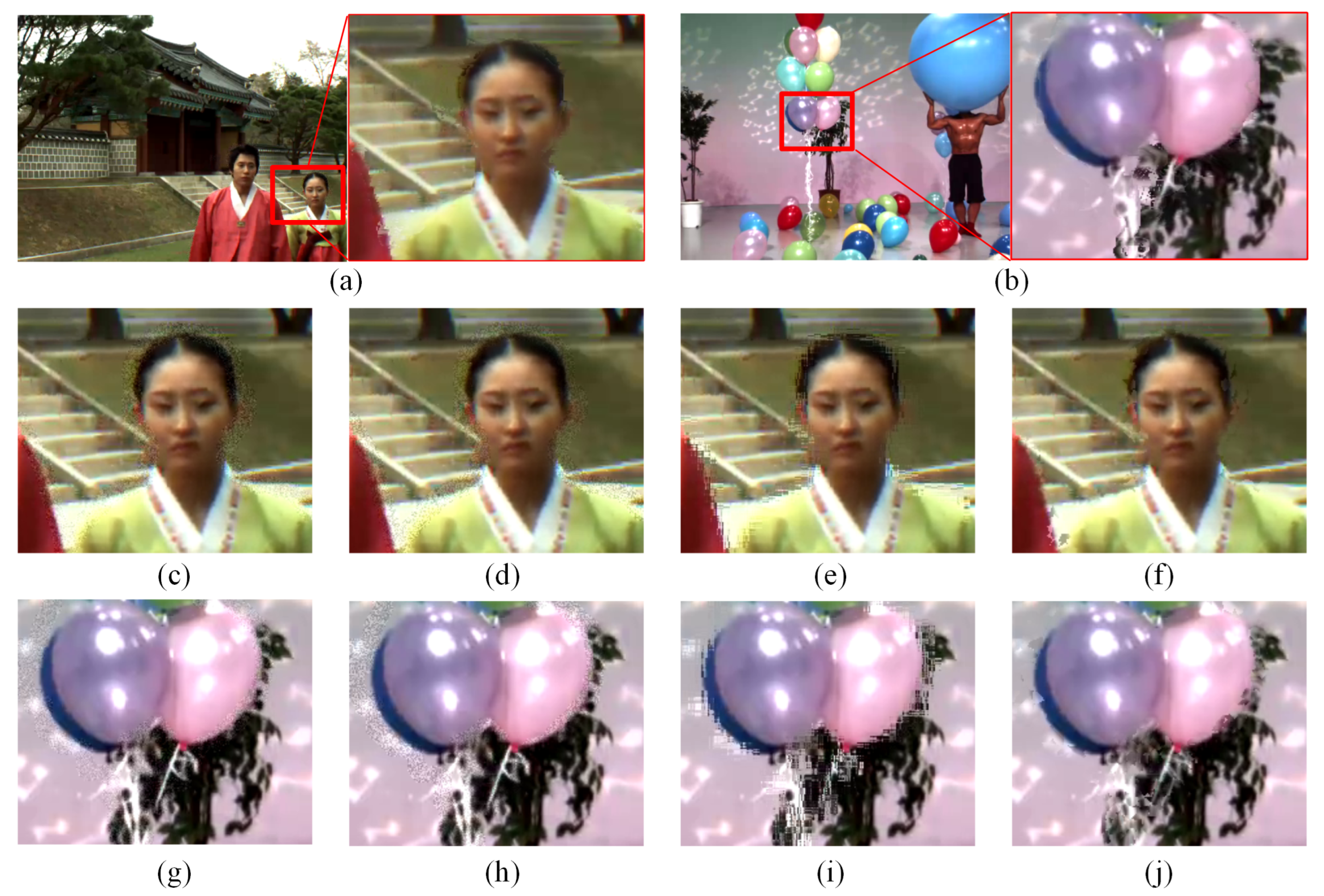
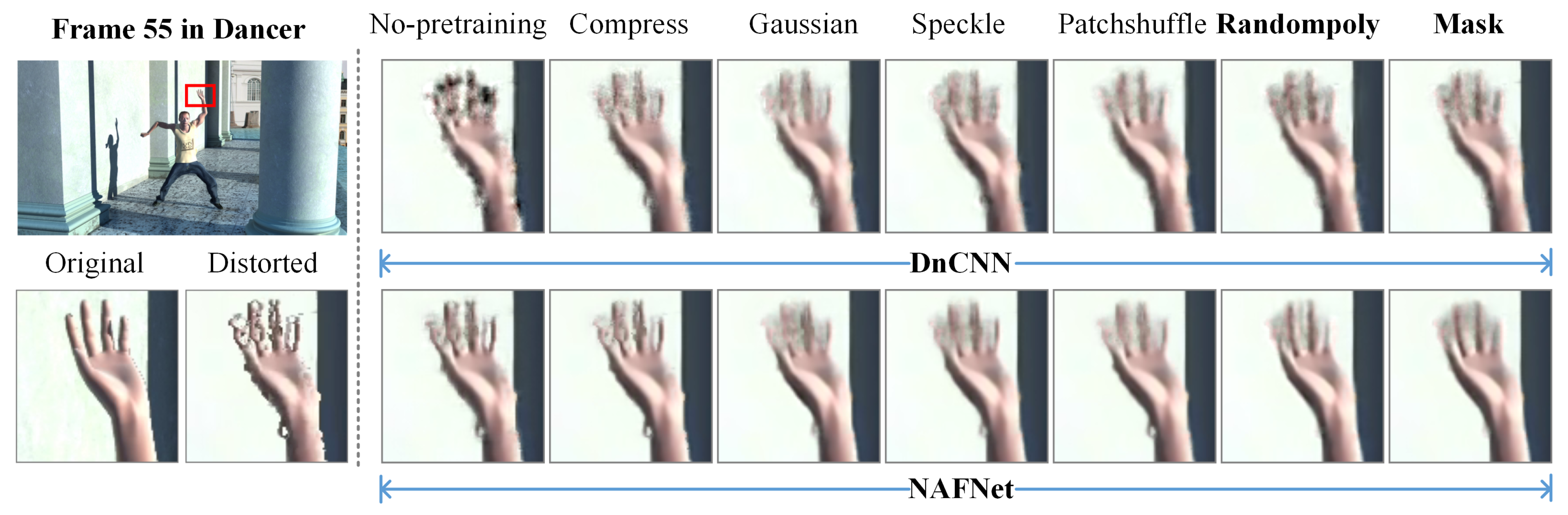
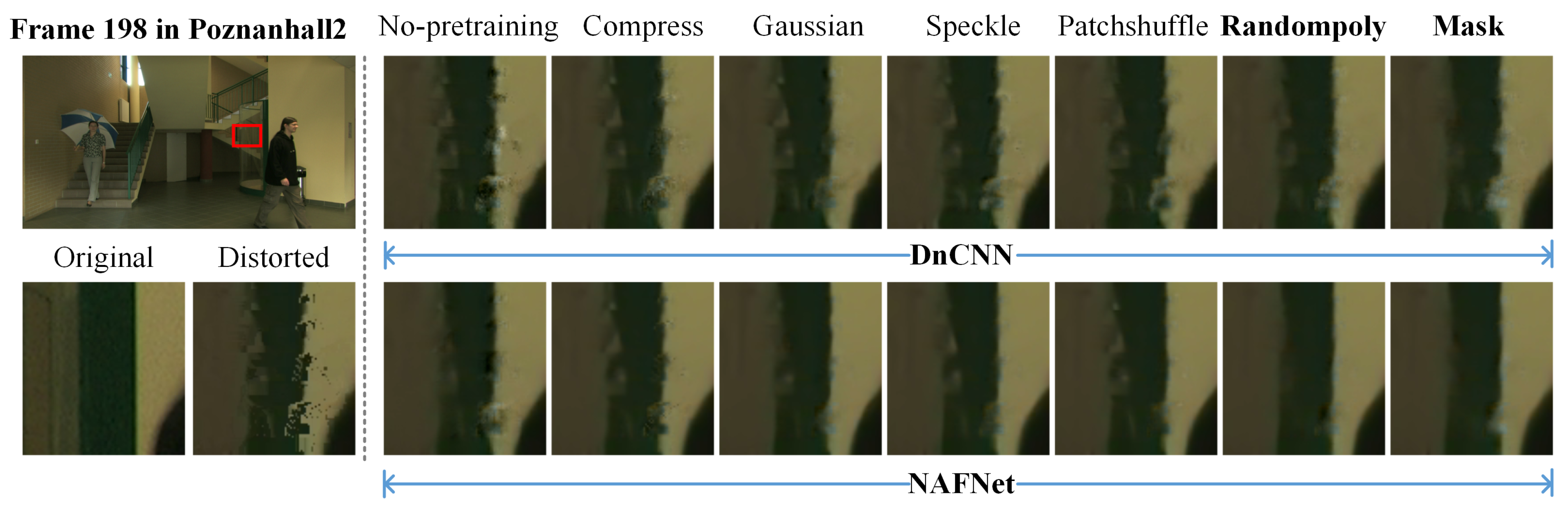
5.2. Verification of Proposed Random Polygon-Based Noise for DIBR Distortion Simulation
5.3. Quantitative Comparisons among SVQE Models Pre-Trained with Synthetic Synthesized Image Database
5.4. Effectiveness of Integrating DIBR Distortion Mask Prediction Sub-Network
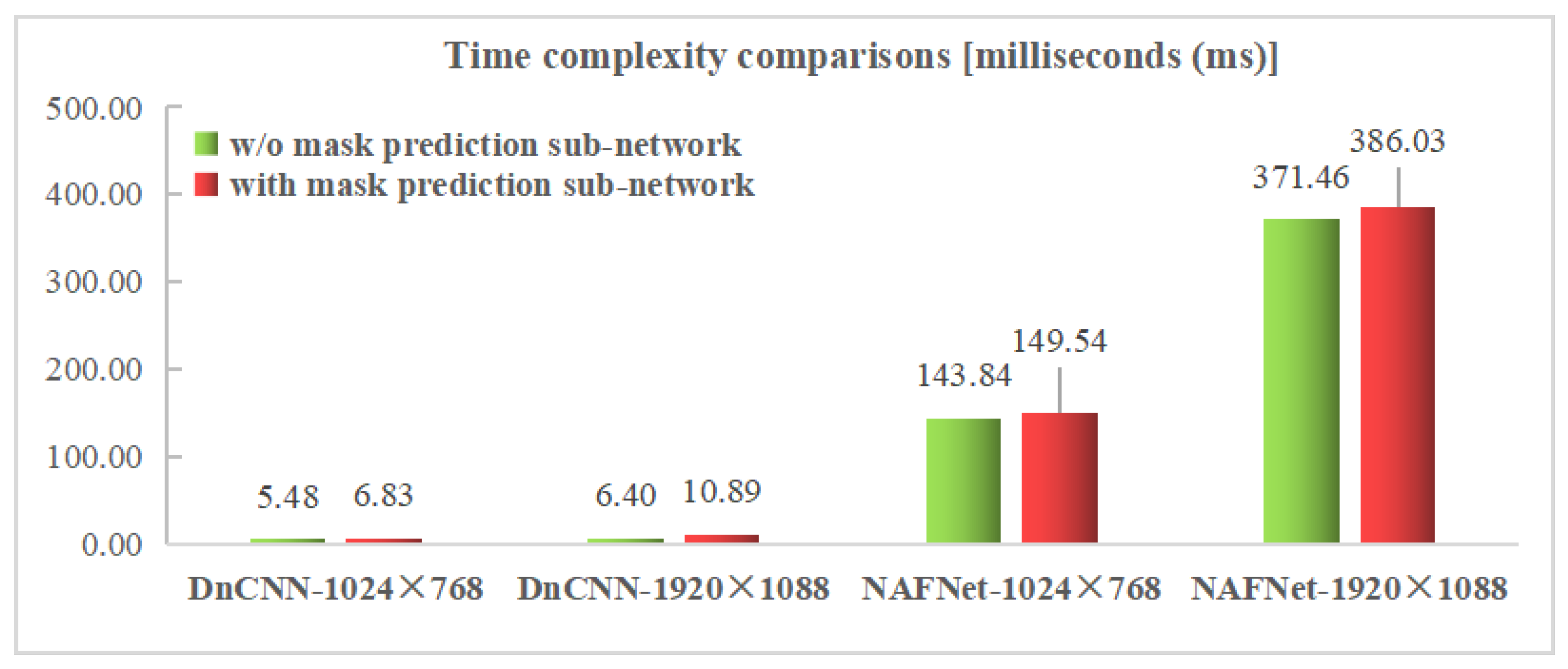
5.5. Computational Complexity Analysis
5.6. Discussion
6. Conclusions
Author Contributions
Funding
Institutional Review Board Statement
Informed Consent Statement
Data Availability Statement
Conflicts of Interest
References
- Zhang, H.; Zhang, Y.; Zhu, L.; Lin, W. Deep learning-based perceptual video quality enhancement for 3D synthesized view. IEEE Trans. Circuits Syst. Video Technol. 2022, 32, 5080–5094. [Google Scholar] [CrossRef]
- Zhang, K.; Zuo, W.; Chen, Y.; Meng, D.; Zhang, L. Beyond a gaussian denoiser: Residual learning of deep CNN for image denoising. IEEE Trans. Image Process. 2017, 26, 3142–3155. [Google Scholar] [CrossRef] [PubMed]
- Guo, S.; Yan, Z.; Zhang, K.; Zuo, W.; Zhang, L. Toward convolutional blind denoising of real photographs. In Proceedings of the 2019 IEEE Conference on Computer Vision and Pattern Recognition (CVPR), Long Beach, CA, USA, 16–20 June 2019; pp. 1712–1722. [Google Scholar] [CrossRef]
- Zhang, Y.; Tian, Y.; Kong, Y.; Zhong, B.; Fu, Y. Residual dense network for image restoration. IEEE Trans. Pattern Anal. Mach. Intell. 2021, 43, 2480–2495. [Google Scholar] [CrossRef] [PubMed]
- Pan, Z.; Yu, W.; Lei, J.; Ling, N.; Kwong, S. TSAN: Synthesized view quality enhancement via two-stream attention network for 3D-HEVC. IEEE Trans. Circuits Syst. Video Technol. 2022, 32, 345–358. [Google Scholar] [CrossRef]
- Pan, Z.; Yuan, F.; Yu, W.; Lei, J.; Ling, N.; Kwong, S. RDEN: Residual distillation enhanced network-guided lightweight synthesized view quality enhancement for 3D-HEVC. IEEE Trans. Circuits Syst. Video Technol. 2022, 32, 6347–6359. [Google Scholar] [CrossRef]
- Buades, A.; Coll, B.; Morel, J. A non-local algorithm for image denoising. In Proceedings of the 2005 IEEE Conference on Computer Vision and Pattern Recognition (CVPR), San Diego, CA, USA, 20–26 June 2005; pp. 60–65. [Google Scholar] [CrossRef]
- Dabov, K.; Foi, A.; Katkovnik, V.; Egiazarian, K. Image denoising by sparse 3-D transformdomain collaborative filtering. IEEE Trans. Image Process. 2007, 16, 2080–2095. [Google Scholar] [CrossRef]
- Zhang, K.; Zuo, W.; Zhang, L. FFDNet: Toward a fast and flexible solution for CNN-based image denoising. IEEE Trans. Image Process. 2018, 27, 4608–4622. [Google Scholar] [CrossRef]
- Chen, L.; Chu, X.; Zhang, X.; Sun, J. Simple baselines for image restoration. arXiv 2022, arXiv:2204.04676. [Google Scholar]
- Zamir, S.W.; Arora, A.; Khan, S.; Hayat, M.; Khan, F.S.; Yang, M. Restormer: Efficient transformer for high-resolution image restoration. In Proceedings of the 2022 IEEE/CVF Conference on Computer Vision and Pattern Recognition (CVPR), New Orleans, LA, USA, 18–24 June 2022; pp. 5718–5729. [Google Scholar] [CrossRef]
- Liang, J.; Cao, J.; Sun, G.; Zhang, K.; Gool, L.V.; Timofte, R. SwinIR: Image restoration using swin transformer. In Proceedings of the 2021 IEEE/CVF International Conference on Computer Vision Workshops, ICCVW, Montreal, BC, Canada, 11–17 October 2021; pp. 1833–1844. [Google Scholar] [CrossRef]
- Dai, Y.; Liu, D.; Wu, F. A convolutional neural network approach for post-processing in HEVC intra coding. In Proceedings of the 23rd International Conference on MultiMedia Modeling (MMM), Reykjavik, Iceland, 4–6 January 2017; pp. 28–39. [Google Scholar] [CrossRef]
- Liu, J.; Zhou, M.; Xiao, M. Deformable convolution dense network for compressed video quality enhancement. In Proceedings of the 2022 IEEE International Conference on Acoustics, Speech and Signal Processing (ICASSP), Singapore, 23–27 May 2022; pp. 1930–1934. [Google Scholar] [CrossRef]
- Yang, R.; Sun, X.; Xu, M.; Zeng, W. Quality-gated convolutional LSTM for enhancing compressed video. In Proceedings of the 2019 IEEE International Conference on Multimedia and Expo (ICME), Shanghai, China, 8–12 July 2019; pp. 532–537. [Google Scholar] [CrossRef]
- Zhu, L.; Zhang, Y.; Wang, S.; Yuan, H.; Kwong, S.; Ip, H.H.S. Convolutional neural network-based synthesized view quality enhancement for 3D video coding. IEEE Trans. Image Process. 2018, 27, 5365–5377. [Google Scholar] [CrossRef]
- Krizhevsky, A.; Sutskever, I.; Hinton, G.E. ImageNet classification with deep convolutional neural networks. In Proceedings of the 26th Annual Conference on Neural Information Processing Systems 2012, Lake Tahoe, NV, USA, 3–6 December 2012; pp. 1106–1114. [Google Scholar]
- Takahashi, R.; Matsubara, T.; Uehara, K. Data augmentation using random image cropping and patches for deep CNNs. IEEE Trans. Circuits Syst. Video Technol. 2020, 30, 2917–2931. [Google Scholar] [CrossRef]
- Summers, C.; Dinneen, M.J. Improved mixed-example data augmentation. In Proceedings of the 2019 IEEE Winter Conference on Applications of Computer Vision (WACV), Waikoloa Village, HI, USA, 7–11 January 2019; pp. 1262–1270. [Google Scholar] [CrossRef]
- Liang, D.; Yang, F.; Zhang, T.; Yang, P. Understanding mixup training methods. IEEE Access 2018, 6, 58774–58783. [Google Scholar] [CrossRef]
- Sixt, L.; Wild, B.; Landgraf, T. RenderGAN: Generating realistic labeled data. In Proceedings of the 5th International Conference on Learning Representations (ICLR), Workshop Track Proceedings, Toulon, France, 24–26 April 2017. [Google Scholar]
- Zhu, J.; Park, T.; Isola, P.; Efros, A.A. Unpaired image-to-image translation using cycle-consistent adversarial networks. In Proceedings of the 2017 IEEE International Conference on Computer Vision (ICCV), Venice, Italy, 22–29 October 2017; pp. 2242–2251. [Google Scholar] [CrossRef]
- Shrivastava, A.; Pfister, T.; Tuzel, O.; Susskind, J.; Wang, W.; Webb, R. Learning from simulated and unsupervised images through adversarial training. In Proceedings of the 2017 IEEE Conference on Computer Vision and Pattern Recognition (CVPR), Honolulu, HI, USA, 21–26 July 2017; pp. 2242–2251. [Google Scholar] [CrossRef]
- Wang, X.; Man, Z.; You, M.; Shen, C. Adversarial generation of training examples: Applications to moving vehicle license plate recognition. arXiv 2017, arXiv:1707.03124. [Google Scholar]
- Chen, P.; Li, L.; Wu, J.; Dong, W.; Shi, G. Contrastive self-supervised pre-training for video quality assessment. IEEE Trans. Image Process. 2022, 31, 458–471. [Google Scholar] [CrossRef] [PubMed]
- Liu, T.; Xu, M.; Wang, Z. Removing rain in videos: A large-scale database and a two-stream ConvLSTM approach. In Proceedings of the 2019 IEEE International Conference on Multimedia and Expo (ICME), Shanghai, China, 8–12 July 2019; pp. 664–669. [Google Scholar] [CrossRef]
- Inoue, N.; Yamasaki, T. Learning from synthetic shadows for shadow detection and removal. IEEE Trans. Circuits Syst. Video Technol. 2021, 31, 4187–4197. [Google Scholar] [CrossRef]
- Cun, X.; Pun, C.; Shi, C. Towards ghost-free shadow removal via dual hierarchical aggregation network and shadow matting GAN. In Proceedings of the 34th AAAI Conference on Artificial Intelligence (AAAI), New York, NY, USA, 7–12 February 2020; pp. 10680–10687. [Google Scholar]
- Madhusudana, P.C.; Birkbeck, N.; Wang, Y.; Adsumilli, B.; Bovik, A.C. Image quality assessment using synthetic images. In Proceedings of the 2022 IEEE/CVF Winter Conference on Applications of Computer Vision Workshops (WACVW), Waikoloa, HI, USA, 4–8 January 2022; pp. 93–102. [Google Scholar] [CrossRef]
- Gupta, A.; Vedaldi, A.; Zisserman, A. Synthetic data for text localisation in natural images. In Proceedings of the 2016 IEEE Conference on Computer Vision and Pattern Recognition (CVPR), Las Vegas, NV, USA, 27–30 June 2016; pp. 2315–2324. [Google Scholar] [CrossRef]
- Li, L.; Huang, Y.; Wu, J.; Gu, K.; Fang, Y. Predicting the quality of view synthesis with color-depth image fusion. IEEE Trans. Circuits Syst. Video Technol. 2021, 31, 2509–2521. [Google Scholar] [CrossRef]
- Ling, S.; Li, J.; Che, Z.; Zhou, W.; Wang, J.; Le Callet, P. Re-visiting discriminator for blind free-viewpoint image quality assessment. IEEE Trans. Multimed. 2021, 23, 4245–4258. [Google Scholar] [CrossRef]
- Zhang, H.; Patel, V.M. Density-aware single image de-raining using a multi-stream dense network. In Proceedings of the 2018 IEEE Conference on Computer Vision and Pattern Recognition (CVPR), Salt Lake City, UT, USA, 18–22 June 2018; pp. 695–704. [Google Scholar] [CrossRef]
- Purohit, K.; Suin, M.; Rajagopalan, A.N.; Boddeti, V.N. Spatially-adaptive image restoration using distortion-guided networks. In Proceedings of the 2021 IEEE/CVF International Conference on Computer Vision (ICCV), Montreal, QC, Canada, 10–17 October 2021; pp. 2289–2299. [Google Scholar] [CrossRef]
- Pan, S.J.; Yang, Q. A survey on transfer learning. IEEE Trans. Knowl. Data Eng. 2010, 22, 1345–1359. [Google Scholar] [CrossRef]
- Silberman, N.; Hoiem, D.; Kohli, P.; Fergus, R. Indoor indoor segmentation and support inference from RGBD images. In Proceedings of the 12th European Conference on Computer Vision (ECCV), Florence, Italy, 7–13 October 2012; pp. 746–760. [Google Scholar]
- Timofte, R.; Gu, S.; Wu, J.; Van Gool, L.; Zhang, L.; Yang, M.H.; Haris, M.; Shakhnarovich, G.; Ukita, N.; Hu, S.; et al. NTIRE 2018 challenge on single image super-resolution: Methods and results. In Proceedings of the 2018 IEEE/CVF Conference on Computer Vision and Pattern Recognition Workshops (CVPRW), Salt Lake City, UT, USA, 18–22 June 2018; pp. 852–863. [Google Scholar] [CrossRef]
- Ranftl, R.; Lasinger, K.; Hafner, D.; Schindler, K.; Koltun, V. Towards robust monocular depth estimation: Mixing datasets for zero-shot cross-dataset transfer. IEEE Trans. Pattern Anal. Mach. Intell. 2022, 44, 1623–1637. [Google Scholar] [CrossRef]
- Shih, M.L.; Su, S.Y.; Kopf, J.; Huang, J.B. 3D photography using context-aware layered depth inpainting. In Proceedings of the 2020 IEEE/CVF Conference on Computer Vision and Pattern Recognition (CVPR), Seattle, WA, USA, 13–19 June 2020; pp. 8025–8035. [Google Scholar] [CrossRef]
- Kang, G.; Dong, X.; Zheng, L.; Yang, Y. Patchshuffle regularization. arXiv 2017, arXiv:1707.07103. [Google Scholar]
- Hada, P.S. Approaches for Generating 2D Shapes. Master’s Dissertation, Department of Computer Science, University of Nevada, Las Vegas, NV, USA, 2014. [Google Scholar]
- Random Polygon Generation. Available online: https://stackoverflow.com/questions/8997099/algorithm-to-generate-random-2d-polygon (accessed on 19 October 2022).
- Li, L.; Zhou, Y.; Gu, K.; Lin, W.; Wang, S. Quality assessment of DIBR-synthesized images by measuring local geometric distortions and global sharpness. IEEE Trans. Multimed. 2018, 20, 914–926. [Google Scholar] [CrossRef]
- Wang, G.; Wang, Z.; Gu, K.; Xia, Z. Blind quality assessment for 3D-synthesized images by measuring geometric distortions and image complexity. In Proceedings of the 2019 IEEE International Conference on Acoustics, Speech and Signal Processing (ICASSP), Brighton, UK, 12–17 May 2019; pp. 4040–4044. [Google Scholar] [CrossRef]
- Wan, Z.; Zhang, B.; Chen, D.; Zhang, P.; Chen, D.; Liao, J.; Wen, F. Bringing old photos back to life. In Proceedings of the 2020 IEEE/CVF Conference on Computer Vision and Pattern Recognition (CVPR), Seattle, WA, USA, 13–19 June 2020; pp. 2744–2754. [Google Scholar] [CrossRef]
- Liu, X.; Zhang, Y.; Hu, S.; Kwong, S.; Kuo, C.C.J.; Peng, Q. Subjective and objective video quality assessment of 3D synthesized views with texture/depth compression distortion. IEEE Trans. Image Process. 2015, 24, 4847–4861. [Google Scholar] [CrossRef] [PubMed]
- Reference Software for 3D-AVC: 3DV-ATM V10.0. Available online: https://hevc.hhi.fraunhofer.de/svn/svn_3DVCSoftware/ (accessed on 19 October 2022).
- VSRS-1D-Fast. Available online: https://hevc.hhi.fraunhofer.de/svn/svn_3DVCSoftware (accessed on 19 October 2022).
- Loshchilov, I.; Hutter, F. SGDR: Stochastic gradient descent with warm restarts. In Proceedings of the 5th International Conference on Learning Representations (ICLR),Workshop Track Proceedings, Toulon, France, 24–26 April 2017. [Google Scholar]
- Wang, Z.; Li, Q. Information content weighting for perceptual image quality assessment. IEEE Trans. Image Process. 2011, 20, 1185–1198. [Google Scholar] [CrossRef] [PubMed]
- Sandić-Stanković, D.; Kukolj, D.; Le Callet, P. Multi–scale synthesized view assessment based on morphological pyramids. Eur. J. Electr. Eng. 2016, 67, 3–11. [Google Scholar] [CrossRef]
- Tian, S.; Zhang, L.; Morin, L.; Déforges, O. SC-IQA: Shift compensation based image quality assessment for DIBR-synthesized views. In Proceedings of the 2018 IEEE Visual Communications and Image Processing (VCIP), Taichung, Taiwan, 9–12 December 2018; pp. 1–4. [Google Scholar] [CrossRef]


| Variables | Descriptions |
|---|---|
| /, , / | The source/target domain, feature space, and source/target learning task, respectively |
| Data samples set, which | |
| Ground truth/distorted image pairs for source/target learning tasks | |
| I, , , | A captured view image, I added with random noise, I added with synthetic geometric distortion generated by the proposed random polygon method, and synthetic synthesized image, respectively |
| M | Mask indicating whether the area in I corresponds to strong depth edges |
| , , n, R | The angle, the radius between the i-th point and assumed center point, and the number of vertices, the average value of radius of the generated random polygon, respectively. |
| , | Random variables indicating the irregularity and spikiness of the generated random polygon, respectively |
| MVD, SVQE, SVI, IQA | Acronyms for Multi-view Video plus Depth, synthesized view quality enhancement, synthesized view image, and image quality assessment, respectively |
| Datasets | Origins/Benchmark | Resolution | Contained Noise | Training | Testing |
|---|---|---|---|---|---|
| Synthetic SVI datasets (for pre-training) | NYU Depth Dataset V2 [36] | 640 × 480 | Compression and synthetic DIBR distortion | 1449 images | / |
| DIV2K [37] | 2K 1 | 750 images | / | ||
| Real MVD dataset | SIAT Database [46] | 1920 × 1088 /1024 × 768 | Compression and DIBR distortion | 94 images | 1200 images |
| Metrics | Models | Kendo | Newspaper | Lovebird1 | Poznanhall2 | Dancer | Outdoor | Poznancarpark | Average |
|---|---|---|---|---|---|---|---|---|---|
| PSNR | w/o pre-train | 33.58 | 29.79 | 31.98 | 34.94 | 30.90 | 33.15 | 30.96 | 32.19 |
| Compress | 34.05 | 29.93 | 32.15 | 35.31 | 31.89 | 33.73 | 31.50 | 32.65 | |
| Gaussian | 34.12 | 29.96 | 32.21 | 35.31 | 31.97 | 33.64 | 31.51 | 32.67 | |
| Speckle | 34.09 | 29.94 | 32.21 | 35.26 | 31.94 | 33.66 | 31.47 | 32.65 | |
| Patch shuffle | 34.19 | 29.88 | 32.16 | 35.31 | 32.16 | 33.75 | 31.50 | 32.71 | |
| Randompoly | 34.09 | 29.93 | 32.18 | 35.29 | 32.17 | 33.73 | 31.49 | 32.70 | |
| IW-SSIM | w/o pre-train | 0.9318 | 0.9095 | 0.9402 | 0.9067 | 0.9332 | 0.9642 | 0.9215 | 0.9296 |
| Compress | 0.9365 | 0.9124 | 0.9420 | 0.9108 | 0.9421 | 0.9679 | 0.9253 | 0.9338 | |
| Gaussian | 0.9355 | 0.9132 | 0.9424 | 0.9098 | 0.9433 | 0.9671 | 0.9249 | 0.9338 | |
| Speckle | 0.9351 | 0.9136 | 0.9427 | 0.9087 | 0.9430 | 0.9675 | 0.9252 | 0.9337 | |
| Patch shuffle | 0.9351 | 0.9136 | 0.9419 | 0.9094 | 0.9448 | 0.9675 | 0.9252 | 0.9339 | |
| Randompoly | 0.9357 | 0.9132 | 0.9425 | 0.9100 | 0.9447 | 0.9678 | 0.9252 | 0.9342 | |
| MPPSNRr | w/o pre-train | 36.62 | 31.53 | 36.05 | 37.73 | 29.40 | 34.42 | 34.27 | 34.29 |
| Compress | 36.98 | 31.98 | 36.58 | 37.82 | 31.99 | 35.10 | 34.79 | 35.03 | |
| Gaussian | 37.05 | 32.07 | 36.58 | 37.71 | 32.38 | 35.02 | 34.79 | 35.09 | |
| Speckle | 37.03 | 32.13 | 36.54 | 37.77 | 32.21 | 34.91 | 34.78 | 35.05 | |
| Patch shuffle | 37.04 | 32.17 | 36.58 | 37.87 | 32.67 | 35.09 | 34.81 | 35.18 | |
| Randompoly | 37.13 | 32.10 | 36.57 | 37.91 | 32.66 | 34.88 | 34.79 | 35.15 | |
| SC-IQA | w/o pre-train | 19.77 | 17.06 | 19.32 | 20.32 | 15.66 | 21.86 | 16.56 | 18.65 |
| Compress | 20.22 | 17.55 | 19.76 | 20.45 | 18.01 | 24.48 | 17.39 | 19.70 | |
| Gaussian | 20.26 | 17.55 | 19.88 | 20.49 | 18.06 | 23.96 | 17.46 | 19.67 | |
| Speckle | 20.17 | 17.49 | 20.06 | 20.43 | 18.20 | 24.07 | 17.37 | 19.68 | |
| Patch shuffle | 20.29 | 17.55 | 19.70 | 20.49 | 18.46 | 24.78 | 17.43 | 19.81 | |
| Randompoly | 20.28 | 17.57 | 19.97 | 20.51 | 18.19 | 24.39 | 17.38 | 19.75 |
| Metrics | Models | Kendo | Newspaper | Lovebird1 | Poznanhall2 | Dancer | Outdoor | Poznancarpark | Average |
|---|---|---|---|---|---|---|---|---|---|
| PSNR | w/o pre-train | 34.00 | 29.86 | 32.32 | 35.39 | 31.28 | 33.42 | 31.50 | 32.54 |
| Compress | 34.30 | 30.02 | 32.30 | 35.43 | 32.19 | 33.90 | 31.66 | 32.83 | |
| Gaussian | 34.16 | 29.96 | 32.27 | 35.45 | 32.49 | 33.86 | 31.62 | 32.83 | |
| Speckle | 34.26 | 29.97 | 32.35 | 35.40 | 32.35 | 33.66 | 31.63 | 32.80 | |
| Patch shuffle | 34.29 | 30.07 | 32.32 | 35.40 | 32.41 | 33.86 | 31.66 | 32.86 | |
| Randompoly | 34.27 | 30.04 | 32.42 | 35.41 | 32.59 | 33.89 | 31.66 | 32.90 | |
| IW-SSIM | w/o pre-train | 0.9386 | 0.9136 | 0.9434 | 0.9151 | 0.9342 | 0.9671 | 0.9245 | 0.9338 |
| Compress | 0.9417 | 0.9156 | 0.9444 | 0.9158 | 0.9454 | 0.9694 | 0.9284 | 0.9373 | |
| Gaussian | 0.9413 | 0.9163 | 0.9448 | 0.9166 | 0.9477 | 0.9691 | 0.9279 | 0.9377 | |
| Speckle | 0.9414 | 0.9158 | 0.9447 | 0.9156 | 0.9463 | 0.9685 | 0.9272 | 0.9371 | |
| Patch shuffle | 0.9413 | 0.9159 | 0.9441 | 0.9156 | 0.9468 | 0.9693 | 0.9280 | 0.9373 | |
| Randompoly | 0.9416 | 0.9164 | 0.9456 | 0.9158 | 0.9488 | 0.9694 | 0.9285 | 0.9380 | |
| MPPSNRr | w/o pre-train | 36.99 | 32.04 | 36.57 | 37.93 | 32.09 | 34.76 | 34.80 | 35.02 |
| Compress | 37.20 | 32.20 | 36.82 | 37.97 | 32.71 | 35.41 | 34.91 | 35.32 | |
| Gaussian | 37.15 | 32.23 | 36.87 | 37.95 | 33.08 | 35.40 | 34.96 | 35.38 | |
| Speckle | 37.22 | 32.23 | 36.86 | 37.95 | 32.97 | 35.44 | 34.84 | 35.36 | |
| Patch shuffle | 37.25 | 32.27 | 36.85 | 37.87 | 33.14 | 35.51 | 34.90 | 35.40 | |
| Randompoly | 37.27 | 32.11 | 36.64 | 38.04 | 33.11 | 35.48 | 34.96 | 35.37 | |
| SC-IQA | w/o pre-train | 20.04 | 17.63 | 20.02 | 20.59 | 17.71 | 23.59 | 17.28 | 19.55 |
| Compress | 20.33 | 17.56 | 20.06 | 20.54 | 18.10 | 24.20 | 17.48 | 19.75 | |
| Gaussian | 20.35 | 17.53 | 20.36 | 20.60 | 18.64 | 24.34 | 17.36 | 19.88 | |
| Speckle | 20.39 | 17.50 | 20.48 | 20.59 | 18.35 | 23.53 | 17.47 | 19.76 | |
| Patch shuffle | 20.46 | 17.57 | 20.04 | 20.59 | 18.43 | 24.51 | 17.48 | 19.87 | |
| Randompoly | 20.55 | 17.61 | 20.34 | 20.65 | 18.97 | 24.30 | 17.50 | 19.99 |
| Metrics | Models | Kendo | Newspaper | Lovebird1 | Poznanhall2 | Dancer | Outdoor | Poznancarpark | Average |
|---|---|---|---|---|---|---|---|---|---|
| PSNR | DnCNN | 33.58 | 29.79 | 31.98 | 34.94 | 30.90 | 33.15 | 30.96 | 32.19 |
| DnCNN-syn-N | 34.09 | 29.93 | 32.18 | 35.29 | 32.17 | 33.73 | 31.49 | 32.70 (+0.51) | |
| DnCNN-syn-D | 34.15 | 29.93 | 32.19 | 35.30 | 32.33 | 33.82 | 31.52 | 32.75 (+0.56) | |
| VRCNN | 33.90 | 29.84 | 32.09 | 35.14 | 31.52 | 33.28 | 31.36 | 32.45 | |
| VRCNN-syn-N | 33.99 | 29.87 | 32.08 | 35.20 | 31.59 | 33.55 | 31.39 | 32.52 (+0.08) | |
| VRCNN-syn-D | 34.13 | 29.94 | 32.12 | 35.24 | 32.03 | 33.75 | 31.44 | 32.66 (+0.21) | |
| TSAN | 33.93 | 29.99 | 32.27 | 35.03 | 31.64 | 33.42 | 31.08 | 32.48 | |
| TSAN-syn-N | 34.12 | 29.88 | 32.16 | 35.32 | 32.48 | 33.84 | 31.40 | 32.74 (+0.26) | |
| TSAN-syn-D | 34.20 | 30.04 | 32.30 | 35.38 | 32.45 | 33.80 | 31.53 | 32.81 (+0.33) | |
| NAFNet | 34.00 | 29.86 | 32.32 | 35.39 | 31.28 | 33.42 | 31.50 | 32.54 | |
| NAFNet-syn-N | 34.27 | 30.04 | 32.42 | 35.41 | 32.59 | 33.89 | 31.66 | 32.90 (+0.36) | |
| NAFNet-syn-D | 34.40 | 30.09 | 32.34 | 35.51 | 32.73 | 34.04 | 31.71 | 32.97 (+0.44) | |
| IW-SSIM | DnCNN | 0.9318 | 0.9095 | 0.9402 | 0.9067 | 0.9332 | 0.9642 | 0.9215 | 0.9296 |
| DnCNN-syn-N | 0.9357 | 0.9132 | 0.9425 | 0.9100 | 0.9447 | 0.9678 | 0.9252 | 0.9342 (+0.0046) | |
| DnCNN-syn-D | 0.9377 | 0.9135 | 0.9436 | 0.9116 | 0.9454 | 0.9681 | 0.9261 | 0.9351 (+0.0056) | |
| VRCNN | 0.9324 | 0.9115 | 0.9406 | 0.9062 | 0.9401 | 0.9662 | 0.9227 | 0.9314 | |
| VRCNN-syn-N | 0.9337 | 0.9121 | 0.9404 | 0.9068 | 0.9408 | 0.9666 | 0.9234 | 0.9320 (+0.0006) | |
| VRCNN-syn-D | 0.9336 | 0.9129 | 0.9410 | 0.9064 | 0.9449 | 0.9675 | 0.9240 | 0.9329 (+0.0015) | |
| TSAN | 0.9330 | 0.9138 | 0.9399 | 0.9066 | 0.9407 | 0.9665 | 0.9209 | 0.9316 | |
| TSAN-syn-N | 0.9330 | 0.9138 | 0.9399 | 0.9130 | 0.9471 | 0.9665 | 0.9270 | 0.93433 (+0.0027) | |
| TSAN-syn-D | 0.9424 | 0.9160 | 0.9445 | 0.9151 | 0.9459 | 0.9686 | 0.9277 | 0.93716 (+0.0055) | |
| NAFNet | 0.9386 | 0.9136 | 0.9434 | 0.9151 | 0.9342 | 0.9671 | 0.9245 | 0.9338 | |
| NAFNet-syn-N | 0.9416 | 0.9164 | 0.9456 | 0.9158 | 0.9488 | 0.9694 | 0.9285 | 0.9380 (+0.0042) | |
| NAFNet-syn-D | 0.9439 | 0.9171 | 0.9452 | 0.9169 | 0.9491 | 0.9702 | 0.9291 | 0.9388 (+0.0050) |
| Metrics | Models | Kendo | Newspaper | Lovebird1 | Poznanhall2 | Dancer | Outdoor | Poznancarpark | Average |
|---|---|---|---|---|---|---|---|---|---|
| MPPSNRr | DnCNN | 36.62 | 31.53 | 36.05 | 37.73 | 29.40 | 34.42 | 34.27 | 34.29 |
| DnCNN-syn-N | 37.13 | 32.10 | 36.57 | 37.91 | 32.66 | 34.88 | 34.79 | 35.15 (+0.86) | |
| DnCNN-syn-D | 37.11 | 31.89 | 36.51 | 37.92 | 33.01 | 35.24 | 34.77 | 35.21 (+0.92) | |
| VRCNN | 36.89 | 32.06 | 36.54 | 37.78 | 31.69 | 34.69 | 34.71 | 34.91 | |
| VRCNN-syn-N | 36.97 | 32.04 | 36.33 | 37.84 | 31.91 | 34.84 | 34.77 | 34.96 (+0.05) | |
| VRCNN-syn-D | 36.96 | 32.22 | 36.64 | 37.79 | 32.89 | 35.44 | 34.71 | 35.24 (+0.33) | |
| TSAN | 36.79 | 32.21 | 36.58 | 37.69 | 32.58 | 35.29 | 34.73 | 35.12 | |
| TSAN-syn-N | 37.28 | 32.23 | 36.64 | 37.82 | 33.39 | 35.38 | 34.84 | 35.37 (+0.24) | |
| TSAN-syn-D | 37.26 | 32.06 | 36.65 | 37.89 | 33.43 | 35.33 | 34.87 | 35.35 (+0.23) | |
| NAFNet | 36.99 | 32.04 | 36.57 | 37.93 | 32.09 | 34.76 | 34.80 | 35.02 | |
| NAFNet-syn-N | 37.27 | 32.11 | 36.64 | 38.04 | 33.11 | 35.48 | 34.96 | 35.37 (+0.25) | |
| NAFNet-syn-D | 37.46 | 32.22 | 36.83 | 38.00 | 33.52 | 35.55 | 34.89 | 35.49 (+0.47) | |
| SC-IQA | DnCNN | 19.77 | 17.06 | 19.32 | 20.32 | 15.66 | 21.86 | 16.56 | 18.65 |
| DnCNN-syn-N | 20.28 | 17.57 | 19.97 | 20.51 | 18.19 | 24.39 | 17.38 | 19.75 (+1.10) | |
| DnCNN-syn-D | 20.30 | 17.58 | 19.95 | 20.47 | 18.31 | 24.01 | 17.37 | 19.71 (+1.06) | |
| VRCNN | 20.11 | 17.46 | 19.51 | 20.27 | 18.14 | 22.88 | 17.30 | 19.38 | |
| VRCNN-syn-N | 20.16 | 17.52 | 19.47 | 20.34 | 17.66 | 24.12 | 17.28 | 19.51 (+0.13) | |
| VRCNN-syn-D | 20.14 | 17.55 | 19.47 | 20.32 | 17.60 | 24.97 | 17.16 | 19.60 (+0.22) | |
| TSAN | 19.88 | 17.59 | 19.50 | 20.28 | 17.34 | 24.53 | 16.78 | 19.42 | |
| TSAN-syn-N | 20.33 | 17.39 | 19.33 | 20.52 | 18.58 | 24.47 | 16.89 | 19.65 (+0.23) | |
| TSAN-syn-D | 20.34 | 17.57 | 19.75 | 20.66 | 18.55 | 23.72 | 17.14 | 19.68 (+0.26) | |
| NAFNet | 20.04 | 17.63 | 20.02 | 20.59 | 17.71 | 23.59 | 17.28 | 19.55 | |
| NAFNet-syn-N | 20.55 | 17.61 | 20.34 | 20.65 | 18.97 | 24.30 | 17.50 | 19.99 (+0.44) | |
| NAFNet-syn-D | 20.65 | 17.60 | 20.04 | 20.74 | 19.15 | 25.05 | 17.59 | 20.12 (+0.57) |
| Models | Kendo | Newspaper | Lovebird1 | Poznanhall2 | Dancer | Outdoor | Poznancarpark | Average |
|---|---|---|---|---|---|---|---|---|
| DnCNN | 33.58 | 29.79 | 31.98 | 34.94 | 30.90 | 33.15 | 30.96 | 32.19 |
| DnCNN-GTmask | 34.35 | 30.13 | 32.16 | 34.60 | 32.61 | 33.59 | 30.85 | 32.61 (+0.42) |
| DnCNN-syn-N | 34.09 | 29.92 | 32.18 | 35.30 | 32.14 | 33.74 | 31.50 | 32.70 |
| DnCNN-syn-GM-N | 35.20 | 30.72 | 32.44 | 35.09 | 33.05 | 34.00 | 31.03 | 33.07 (+0.37) |
| DnCNN-syn-D | 34.12 | 29.91 | 32.16 | 35.32 | 32.29 | 33.79 | 31.53 | 32.73 |
| DnCNN-syn-GM-D | 35.35 | 30.83 | 32.51 | 34.92 | 33.22 | 34.17 | 30.86 | 33.12 (+0.39) |
| Model | PSNR | IW-SSIM | MPPSNRr | SC-IQA |
|---|---|---|---|---|
| DnCNN-syn-N | 32.70 | 0.9342 | 35.148 | 19.75 |
| DnCNN-syn-mask-N | 32.72 | 0.9341 | 35.152 | 19.80 |
| DnCNN-syn-D | 32.75 | 0.9352 | 35.208 | 19.71 |
| DnCNN-syn-mask-D | 32.78 | 0.9345 | 35.264 | 19.82 |
| NAFNet-syn-N | 32.90 | 0.9380 | 35.372 | 19.99 |
| NAFNet-syn-mask-N | 32.93 | 0.9380 | 35.493 | 20.00 |
| NAFNet-syn-D | 32.97 | 0.9388 | 35.493 | 20.12 |
| NAFNet-syn-mask-D | 32.98 | 0.9388 | 35.528 | 20.08 |
| Database | Gaussian | Speckle | Patch shuffle | Randompoly |
|---|---|---|---|---|
| NYU Depth Dataset V2 | 67.90 | 65.61 | 76.45 | 1268.82 |
Publisher’s Note: MDPI stays neutral with regard to jurisdictional claims in published maps and institutional affiliations. |
© 2022 by the authors. Licensee MDPI, Basel, Switzerland. This article is an open access article distributed under the terms and conditions of the Creative Commons Attribution (CC BY) license (https://creativecommons.org/licenses/by/4.0/).
Share and Cite
Zhang, H.; Cao, J.; Zheng, D.; Yao, X.; Ling, B.W.-K. Deep Learning-Based Synthesized View Quality Enhancement with DIBR Distortion Mask Prediction Using Synthetic Images. Sensors 2022, 22, 8127. https://doi.org/10.3390/s22218127
Zhang H, Cao J, Zheng D, Yao X, Ling BW-K. Deep Learning-Based Synthesized View Quality Enhancement with DIBR Distortion Mask Prediction Using Synthetic Images. Sensors. 2022; 22(21):8127. https://doi.org/10.3390/s22218127
Chicago/Turabian StyleZhang, Huan, Jiangzhong Cao, Dongsheng Zheng, Ximei Yao, and Bingo Wing-Kuen Ling. 2022. "Deep Learning-Based Synthesized View Quality Enhancement with DIBR Distortion Mask Prediction Using Synthetic Images" Sensors 22, no. 21: 8127. https://doi.org/10.3390/s22218127
APA StyleZhang, H., Cao, J., Zheng, D., Yao, X., & Ling, B. W.-K. (2022). Deep Learning-Based Synthesized View Quality Enhancement with DIBR Distortion Mask Prediction Using Synthetic Images. Sensors, 22(21), 8127. https://doi.org/10.3390/s22218127