Transmission Line Sag Measurement and Simulation Research Based on Non-Contact Electric Field Sensing


Abstract
:1. Introduction
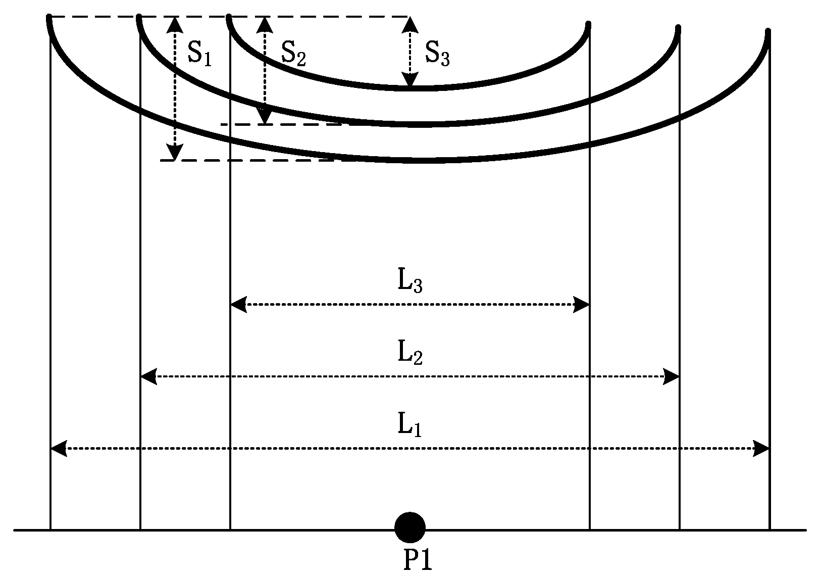
2. Sag Measurement Principle
2.1. Electrostatic Coupling Model between Transmission Line and Measuring Points
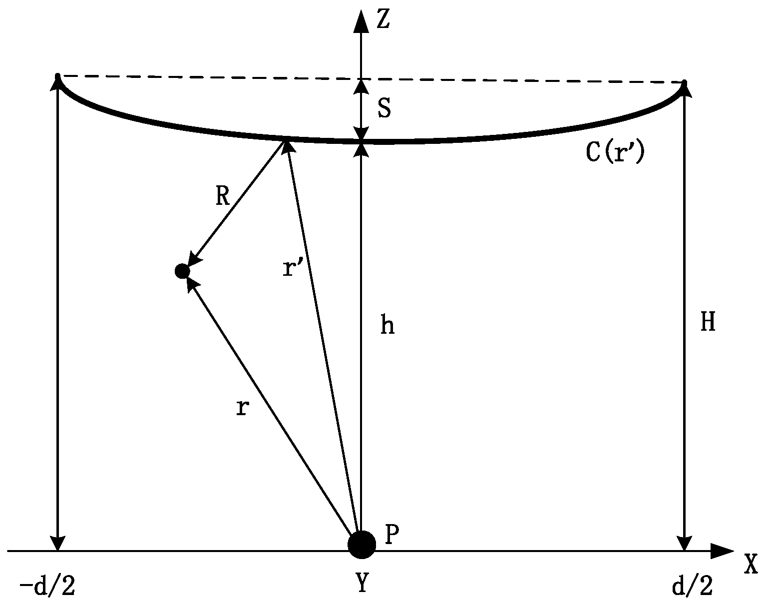
2.1.1. Catenary Line
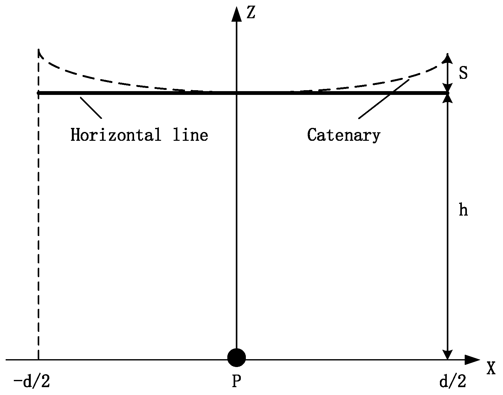
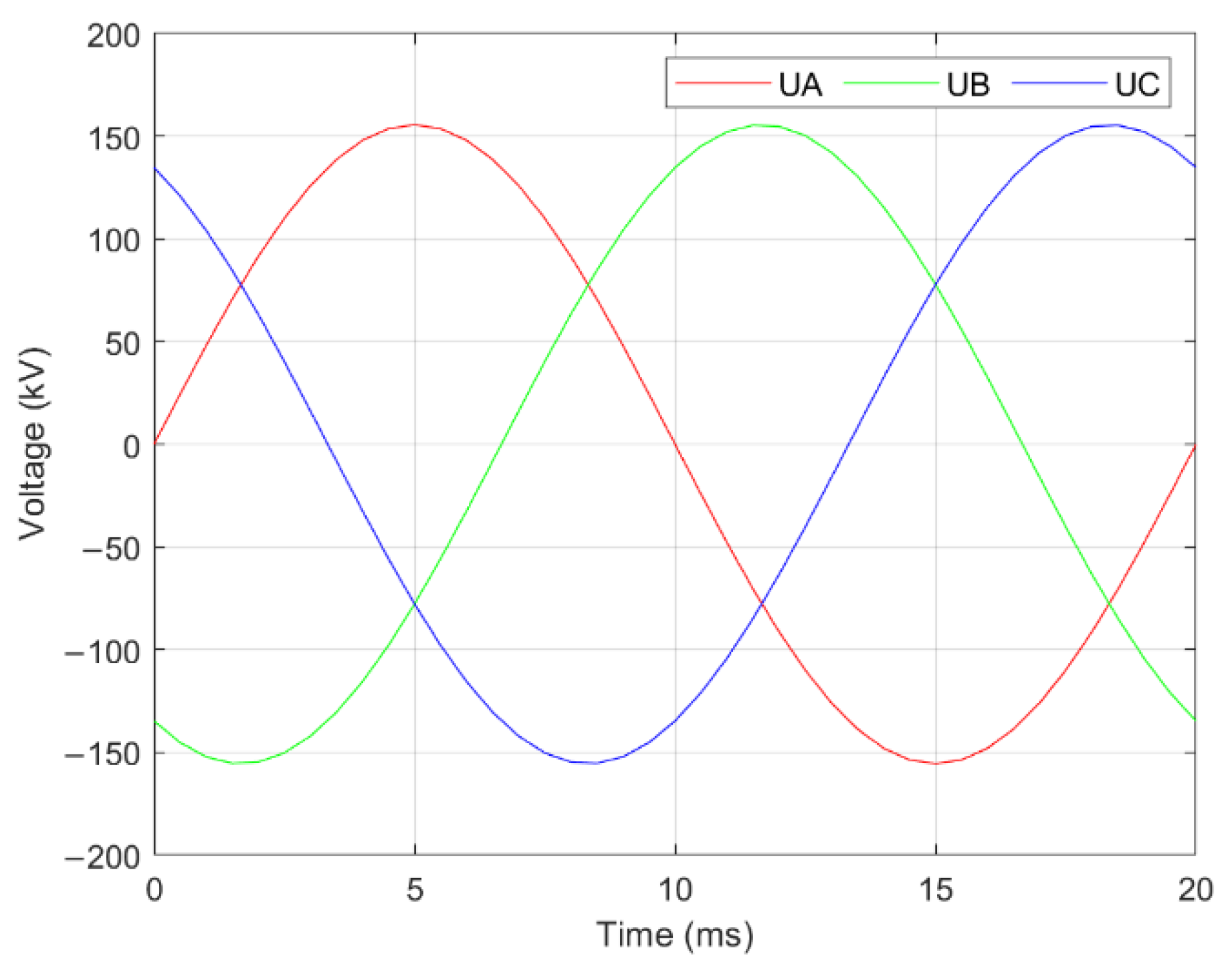
2.1.2. Horizontal Line
2.2. Inverse Calculation of Sag
2.2.1. Theory
2.2.2. Simplified Computing Model
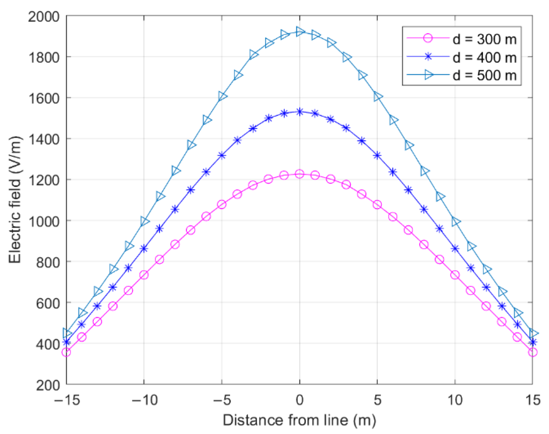
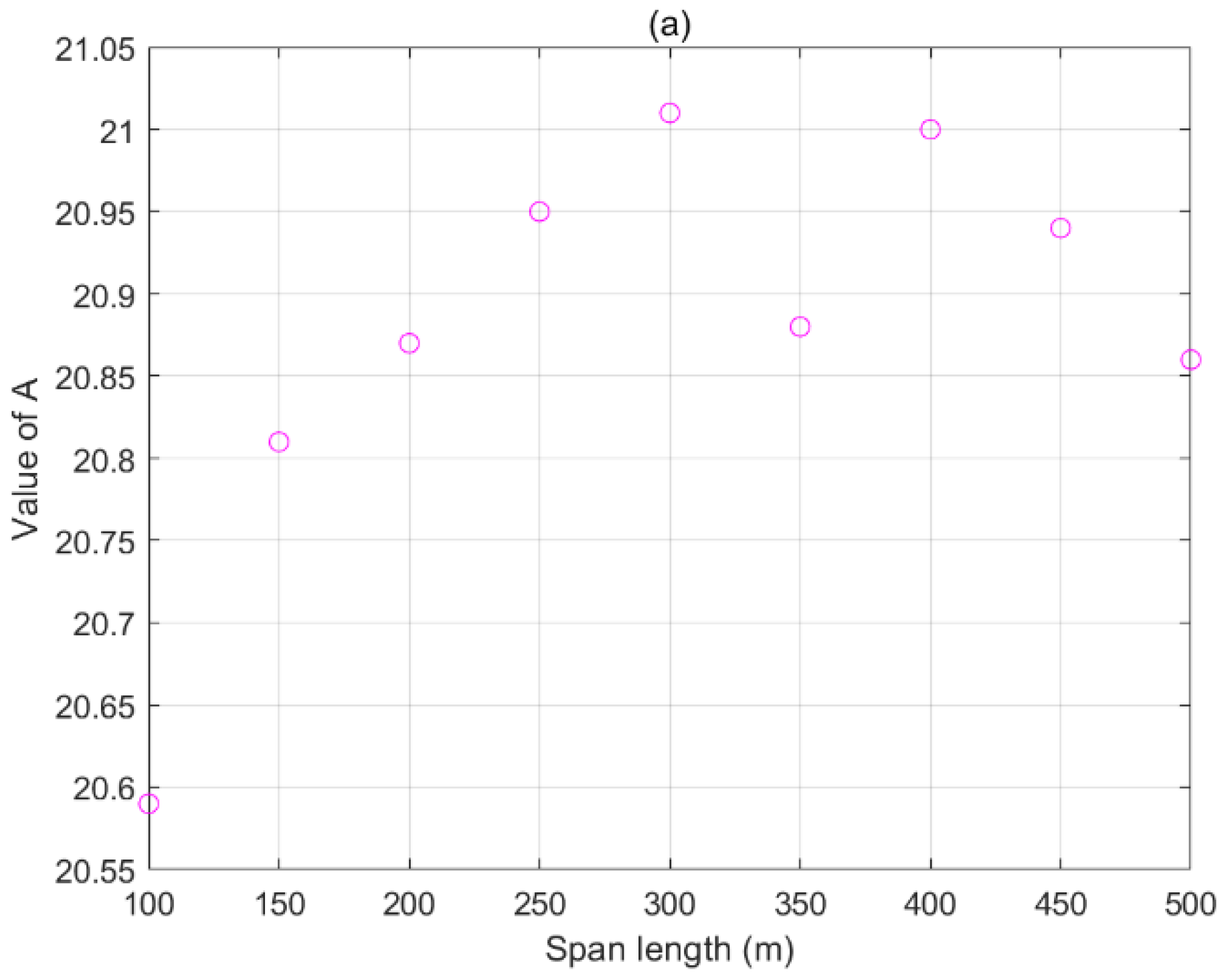
3. Effects of Line Parameters on Sag Measurement
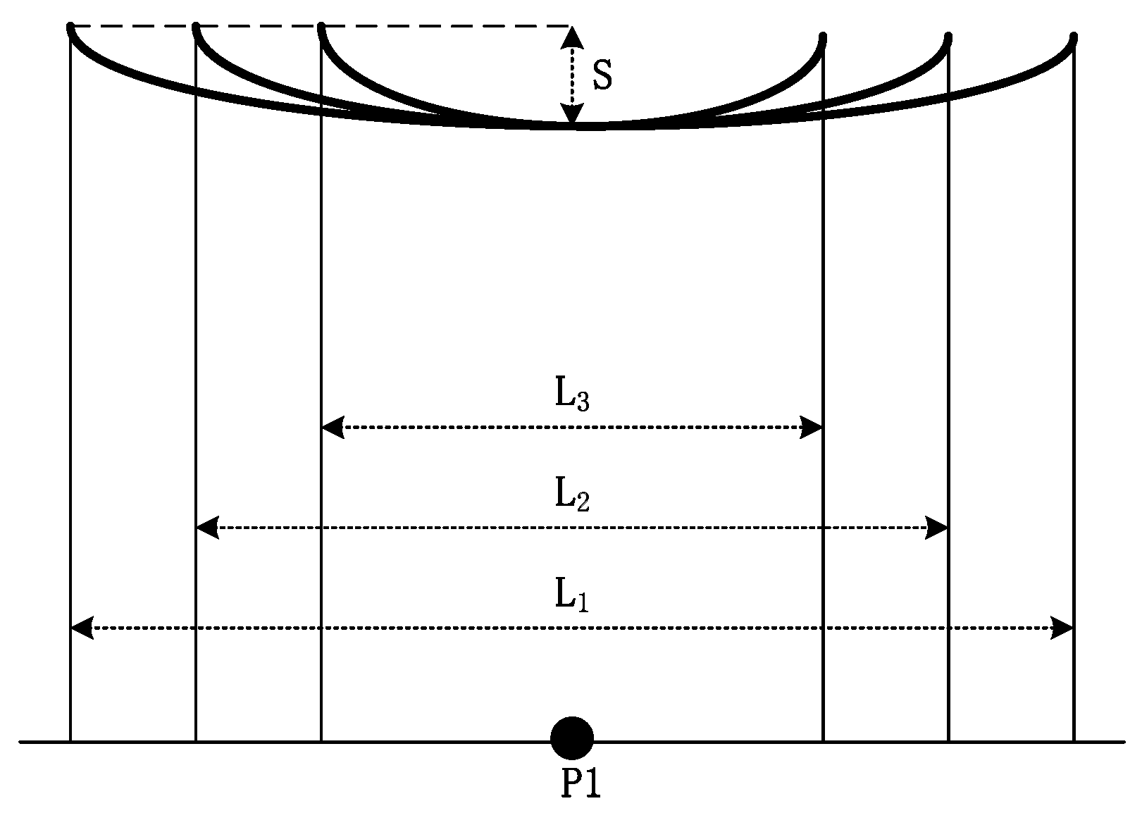
3.1. Span Length
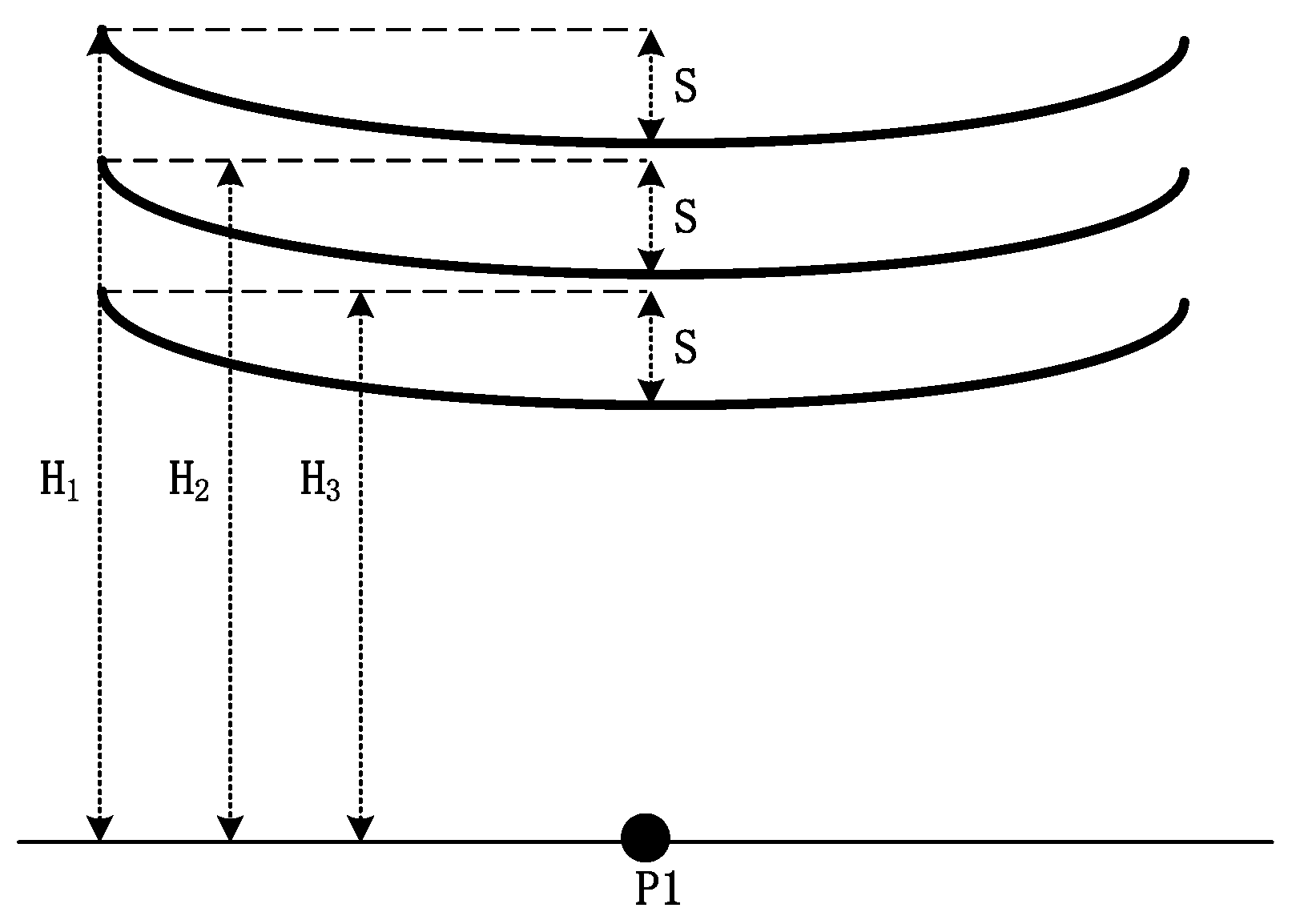
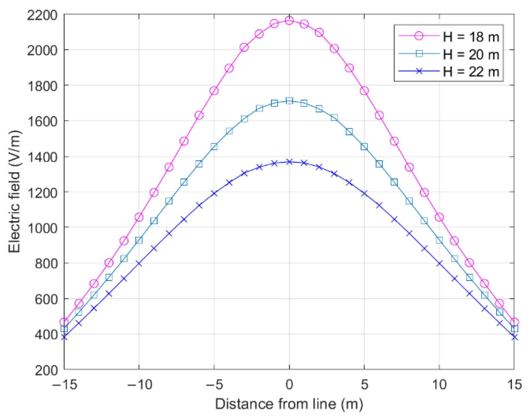
3.2. Tower Height
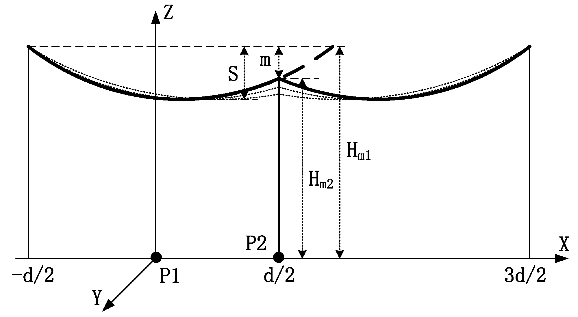
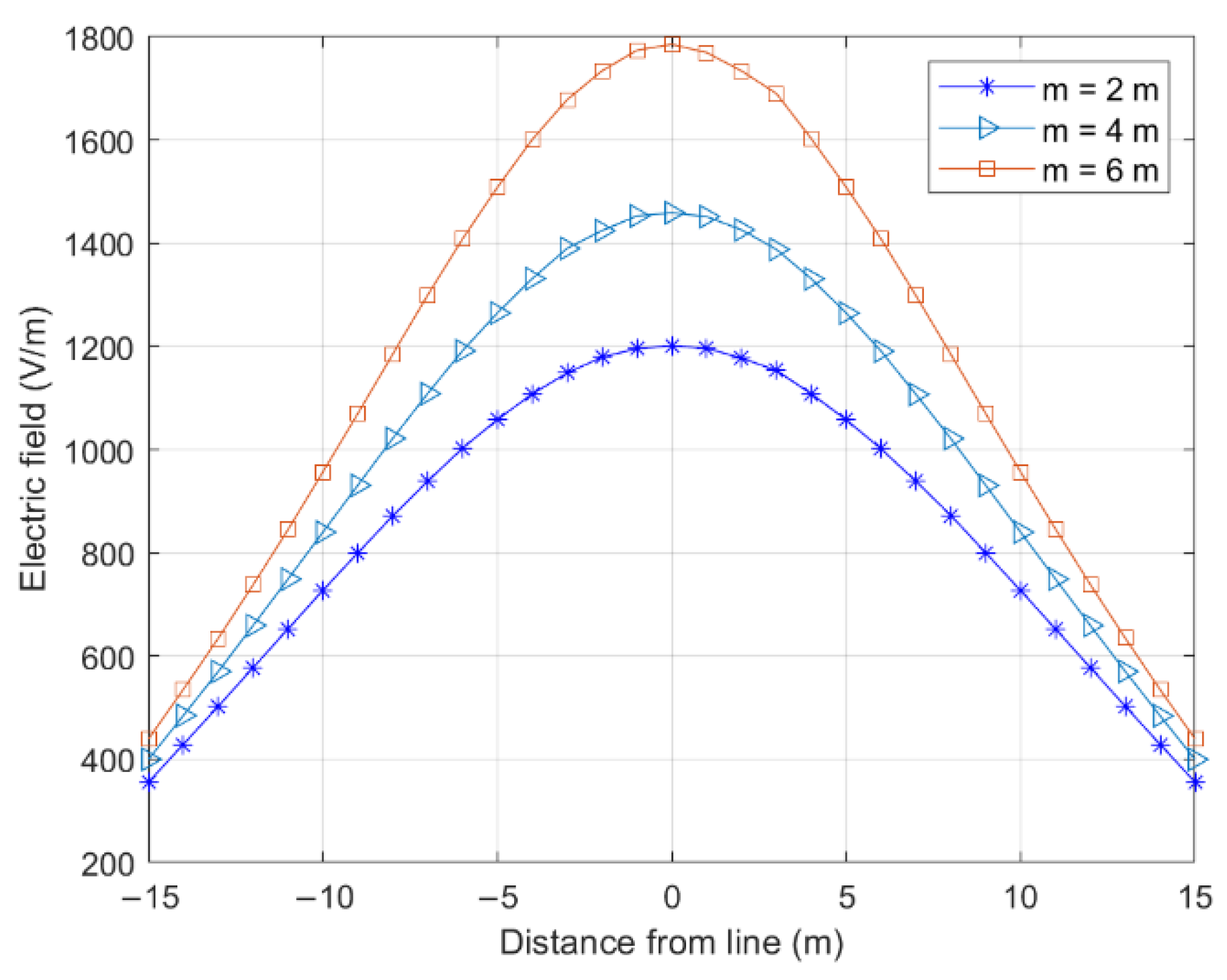
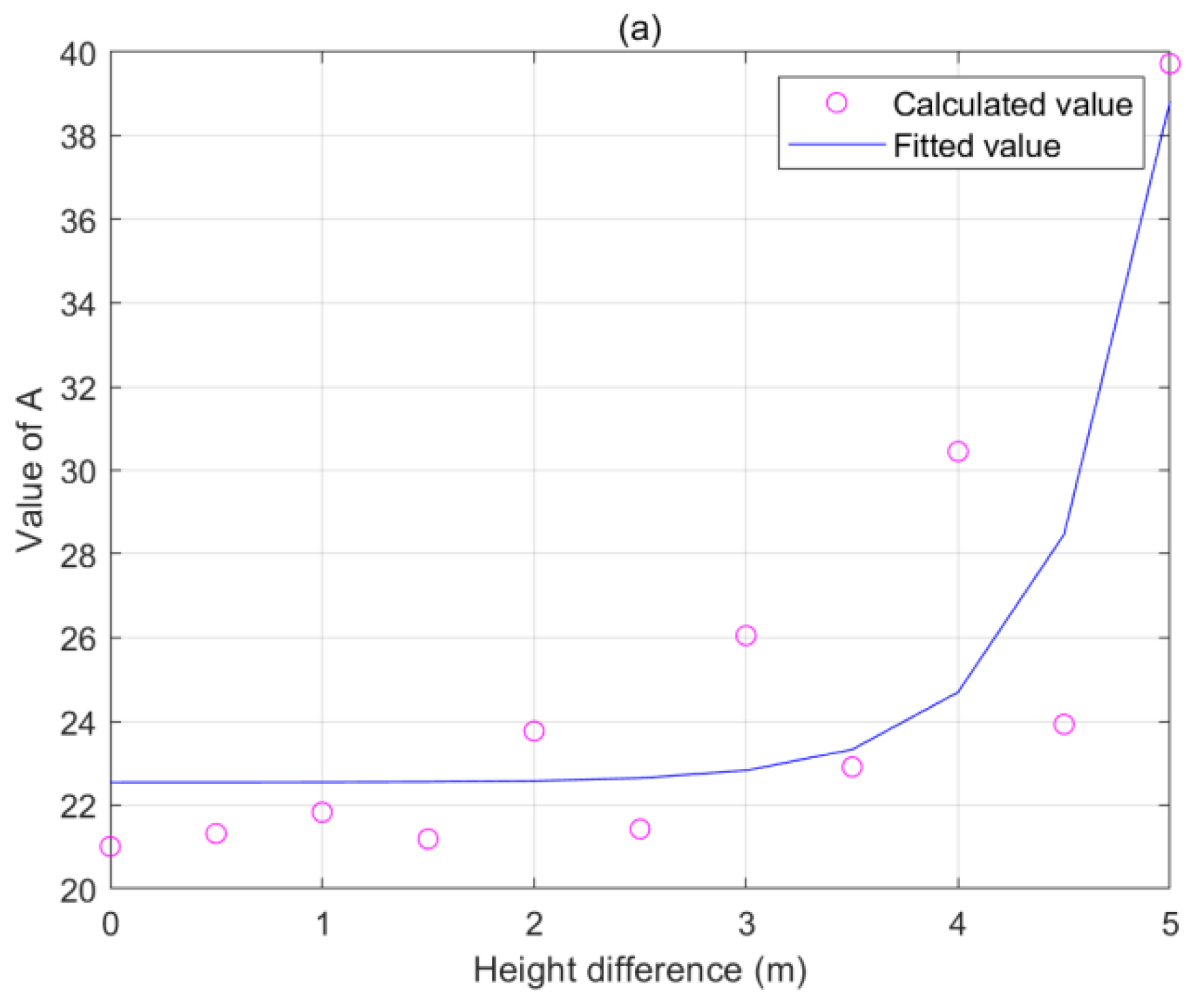
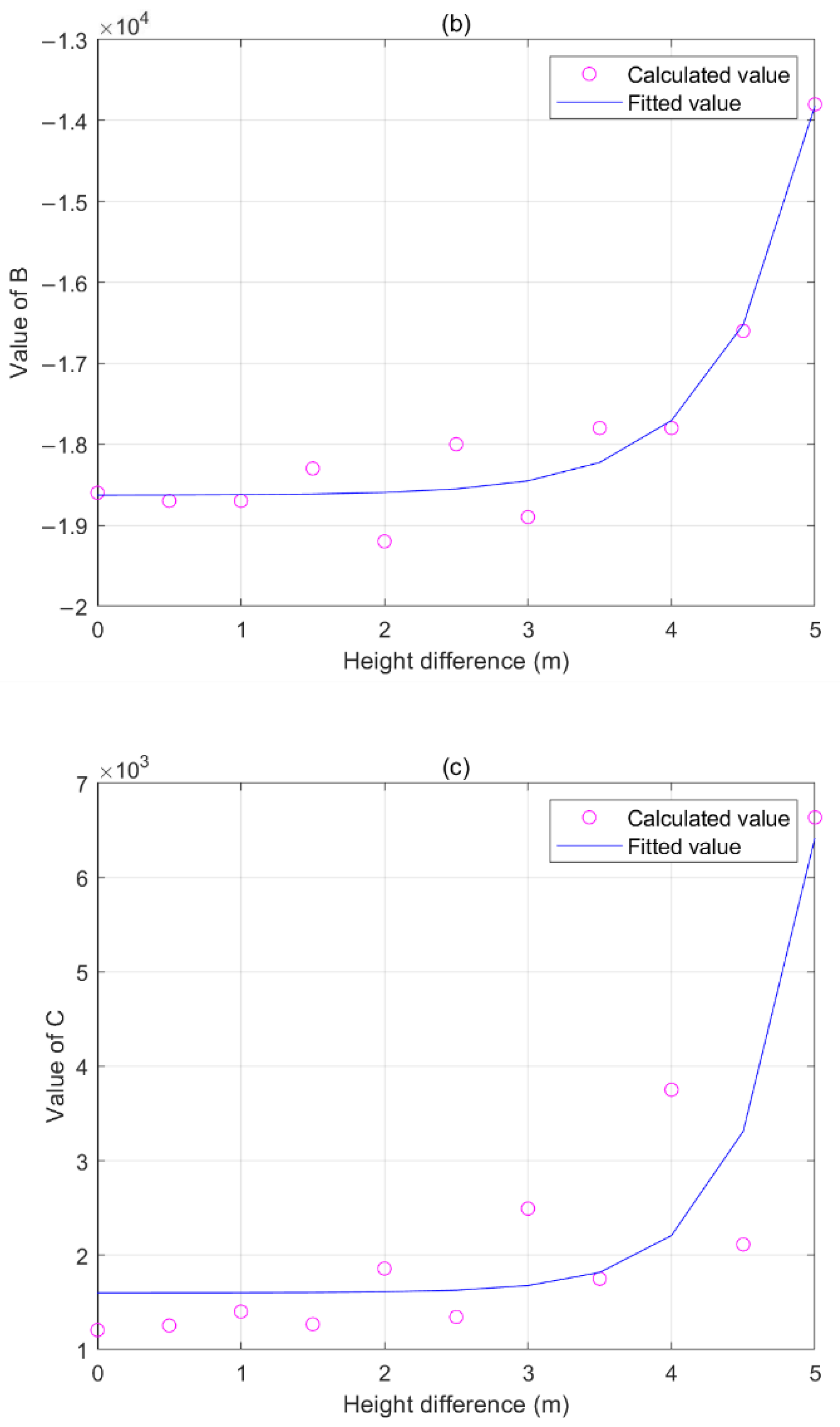
3.3. Tower Height Difference
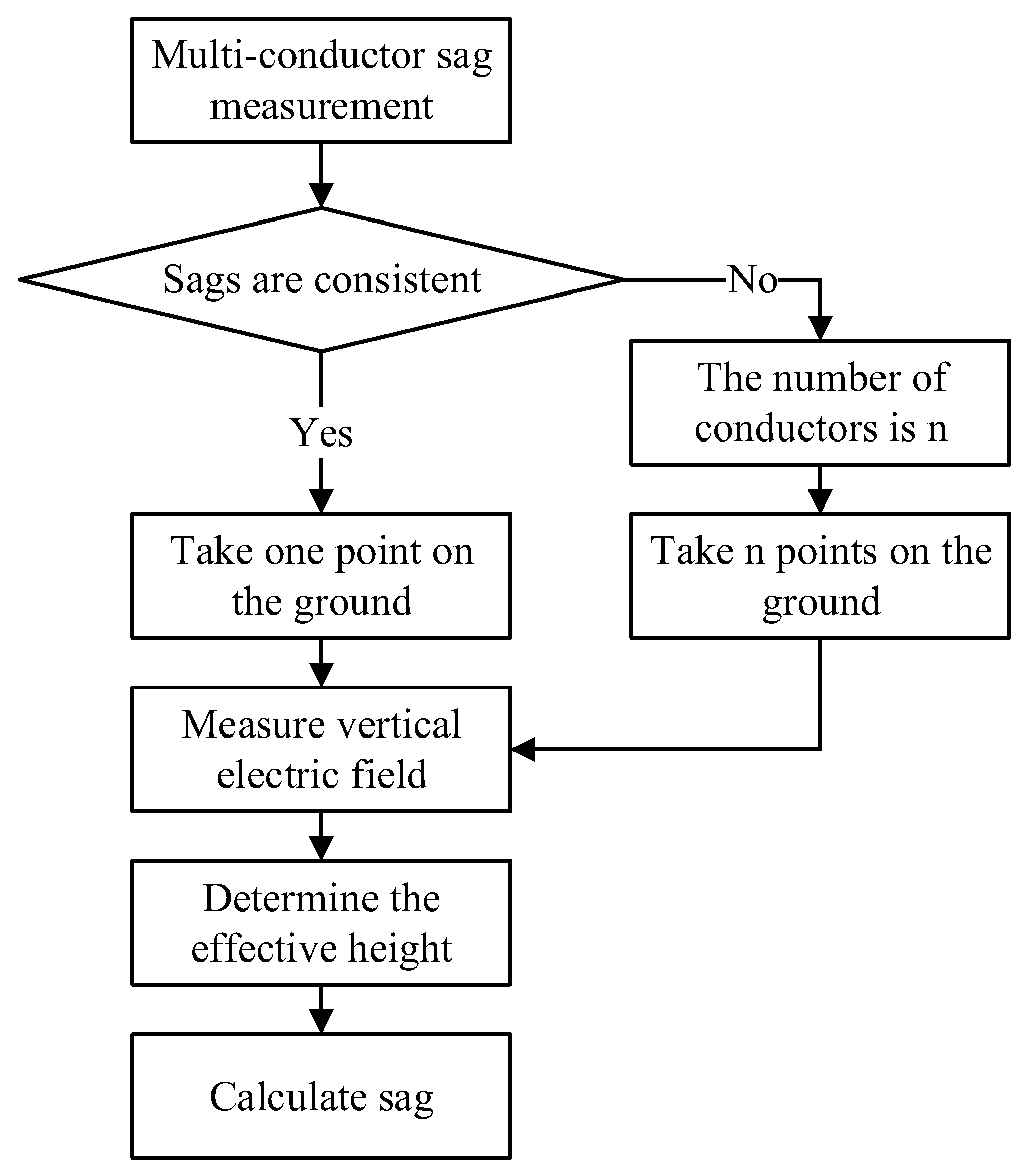
4. Multi-Conductor Sag Measurement
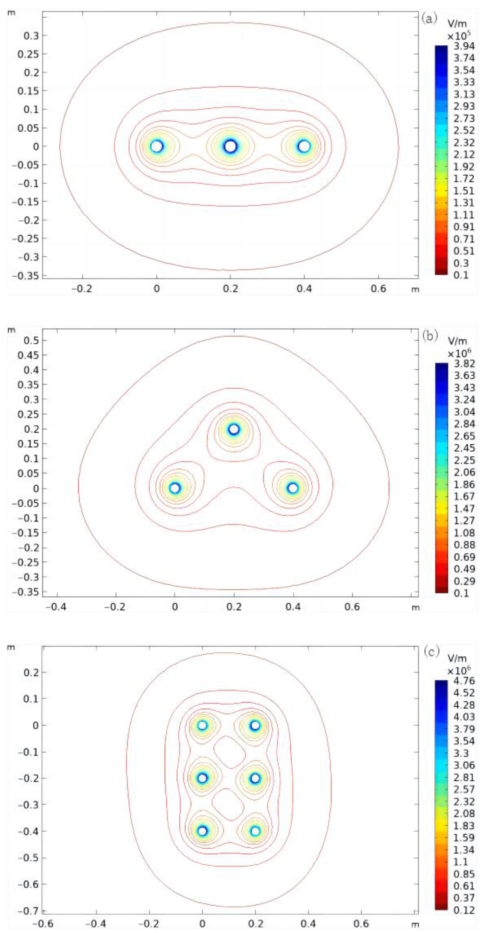
4.1. Arrangement
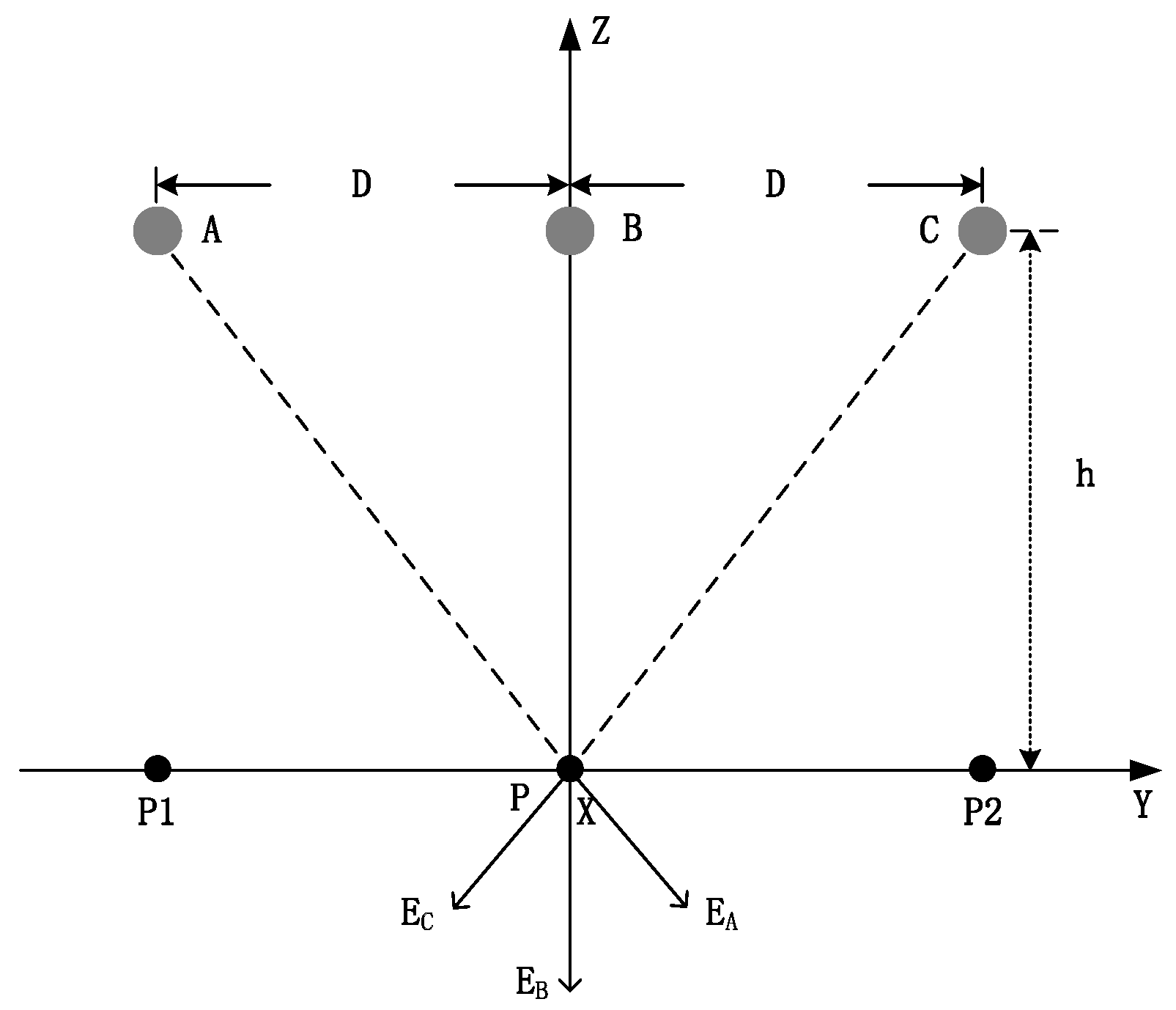
4.2. Single-Round Lines
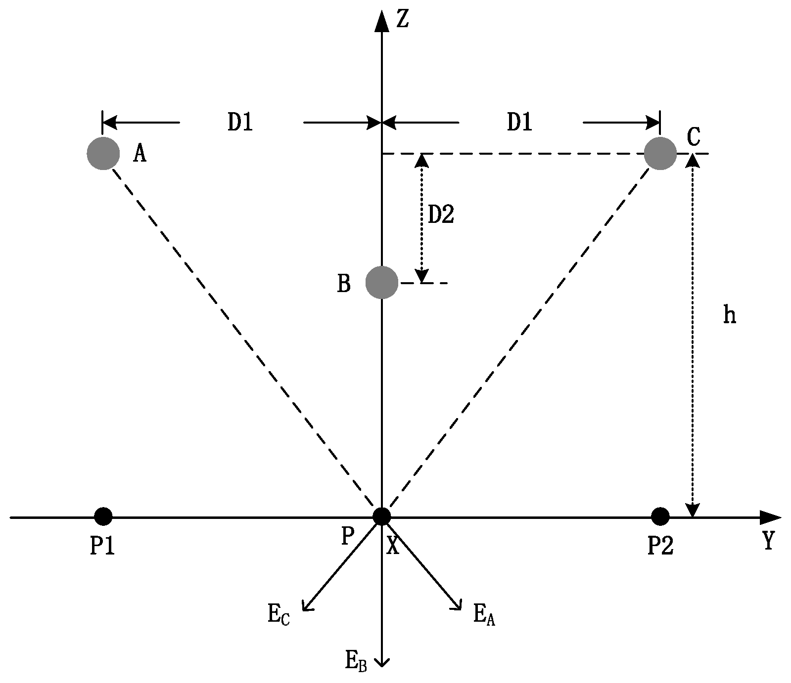
4.3. Dual-Round Lines
5. Conclusions
Author Contributions
Funding
Data Availability Statement
Conflicts of Interest
References
- Wu, Y.; Zhao, G.; Hu, J.; Ouyang, Y.; Wang, S.X.; He, J.; Gao, F.; Wang, S. Overhead Transmission line parameter reconstruction for UAV Inspection based on Tunneling magnetoresistive sensors and Inverse models. IEEE Trans. Power Deliv. 2019, 34, 819–827. [Google Scholar] [CrossRef]
- Khawaja, A.H.; Huang, Q.; Khan, Z.H. Monitoring of Overhead Transmission Lines: A Review from the Perspective of Contactless Technologies. Sens. Imaging 2017, 18, 24. [Google Scholar] [CrossRef]
- Zhang, F.; Fan, M.; Yu, X.; Dong, X.; Wang, W. Forecast Model of Transmission Line Sag Based on GA. J. Phys. Conf. Ser. 2022, 2158, 12008. [Google Scholar] [CrossRef]
- Bao, J.; Wang, X.; Zheng, Y.; Zhang, F.; Huang, X.; Sun, P.; Li, Z. Resilience-Oriented Transmission Line Fragility Modeling and Real-Time Risk Assessment of Thunderstorms. IEEE Trans. Power Deliv. 2021, 36, 2363–2373. [Google Scholar] [CrossRef]
- Omeje, C.O.; Uhunmwangho, R. Sag and Tension Evaluation of a 330 kV Overhead Transmission Line Network for Upland and Level land Topographies. Int. J. Sci. Eng. Res 2020, 11, 229–234. [Google Scholar]
- Malhara, S. Mechanical State Estimation of Transmission Line Sag Using Tilt Sensors. Ph.D. Thesis, Arizona State University, Tempe, AZ, USA, 2009. [Google Scholar]
- Seppa, T.O. Accurate Ampacity Determination: Temperature-Sag Model for Operational Real Time Ratings. IEEE Trans. Power Deliv. 1995, 10, 1460–1470. [Google Scholar] [CrossRef]
- Prasetyo, H.; Sudiarto, B.; Setiabudy, R. Analysis of Knee Point Temperature (KPT) determination on High Capacity Low Sag (HCLS) conductors for optimizing the ampacity load and sag on the overhead transmission lines system. IOP Conf. Ser. Mater. Sci. Eng. 2021, 1098, 42021. [Google Scholar] [CrossRef]
- Kamboj, S.; Dahiya, R. Designing and Implementation of Overhead Conductor Altitude Measurement System Using GPS for Sag Monitoring. In Intelligent Computing Techniques for Smart Energy Systems; Springer: Singapore, 2020; Volume 607, pp. 183–194. [Google Scholar] [CrossRef]
- Mahajan, S.M.; Singareddy, U.M. A Real-time conductor sag measurement system using a Differential GPS. IEEE Trans. Power Deliv. 2012, 27, 475–480. [Google Scholar] [CrossRef]
- Shivani, P.G.; Harshit, S.; Varma, C.V.; Mahalakshmi, R. Detection of Icing and Calculation of Sag of Transmission Line through Computer Vision. In Proceedings of the 2020 Third International Conference on Smart Systems and Inventive Technology (ICSSIT), Tirunelveli, India, 22 August 2020. [Google Scholar]
- Wydra, M.; Kisała, P.; Harasim, D.; Kacejko, P. Overhead Transmission Line Sag Estimation Using a Simple Optomechanical System with Chirped Fiber Bragg Gratings. Part 1: Preliminary Measurements. Sensors 2018, 18, 309. [Google Scholar] [CrossRef] [Green Version]
- Skorupski, K.; Harasim, D.; Panas, P.; Cięszczyk, S.; Kisała, P.; Kacejko, P.; Mroczka, J.; Wydra, M. Overhead Transmission Line Sag Estimation Using the Simple Opto-Mechanical System with Fiber Bragg Gratings—Part 2: Interrogation System. Sensors 2020, 20, 2652. [Google Scholar] [CrossRef]
- Zengin, A.T.; Erdemir, G.; Akinci, T.C.; Seker, S. Measurement of Power line sagging using sensor data of a Power line inspection robot. IEEE Access 2020, 8, 99198–99204. [Google Scholar] [CrossRef]
- Yuan, J.; Lei, Y.; Xiong, X. A Contractless Overvoltage Measurement Method Based on the Principle of Multi Conductor Electrostatic Coupling. Trans. China Electrotech. Societa. 2014, 29, 524–530. [Google Scholar]
- Huang, Q.; Song, Y.; Sun, X.; Jiang, L.; Pong, P.W.T. Magnetics in Smart Grid. IEEE Trans. Magn. 2014, 50, 900107. [Google Scholar] [CrossRef] [Green Version]
- Liu, X.; Liu, C.; Pong, P.W.T. Velocity Measurement Technique for Permanent Magnet Synchronous Motors through External Stray Magnetic Field Sensing. IEEE Sens. J. 2018, 18, 4013–4021. [Google Scholar] [CrossRef]
- Khawaja, A.H.; Huang, Q. Estimating Sag and Wind-Induced Motion of Overhead Power Lines with Current and Magnetic-Flux Density Measurements. IEEE Trans. Instrum. Meas. 2017, 66, 897–909. [Google Scholar] [CrossRef]
- Khawaja, A.H.; Huang, Q.; Li, J.; Zhang, Z. Estimation of Current and Sag in Overhead power transmission lines with Optimized magnetic field sensor array placement. IEEE Trans. Magn. 2017, 53, 6100210. [Google Scholar] [CrossRef]
- Xu, Q.; Liu, X.; Zhu, K.; Pong, P.W.T.; Liu, C. Magnetic-Field-Sensing-Based Approach for Current reconstruction, sag detection, and Inclination detection for Overhead transmission system. IEEE Trans. Magn. 2019, 55, 4003307. [Google Scholar] [CrossRef]
- Chen, K.L. Contactless Phase comparison method for Overhead transmission lines. IEEE Sens. J. 2020, 21, 6998–7005. [Google Scholar] [CrossRef]
- El Dein, A.Z.; Wahab, M.A.A.; Hamada, M.M.; Emmary, T.H. The Effects of the Span configurations and Conductor sag on the Electric-field distribution under overhead transmission lines. IEEE Trans. Power Deliv. 2010, 25, 2891–2902. [Google Scholar] [CrossRef]
- Xiao, D.; He, T.; Zhao, W.; Du, X.; Xie, Y. Improved Three-Dimension Mathematical Model for Voltage Inversion of AC Overhead Transmission Lines. IEEE Access 2019, 7, 166740–166748. [Google Scholar] [CrossRef]
- Mukherjee, M.; Olsen, R.G.; Li, Z. Non-contact Monitoring of Overhead transmission lines using space potential phaser measurements. IEEE Trans. Instrum. Meas. 2020, 69, 7494–7504. [Google Scholar] [CrossRef]
- Ji, Y.; Yuan, J. Overhead Transmission lines sag and Voltage monitoring method based on Electrostatic inverse calculation. IEEE Trans. Instrum. Meas. 2022, 71, 9002312. [Google Scholar] [CrossRef]
- Zhu, K.; Lee, W.K.; Pong, P.W.T. Non-Contact Voltage Monitoring of HVDC Transmission Lines Based on Electromagnetic Fields. IEEE Sens. J. 2019, 19, 3121–3129. [Google Scholar] [CrossRef]
- Chen, K.-L.; Guo, Y.; Wang, J.; Yang, X. Contactless Islanding Detection Method Using Electric Field Sensors. IEEE Trans. Instrum. Meas. 2020, 70, 9001413. [Google Scholar] [CrossRef]
- Tsang, K.; Chan, W. Dual capacitive sensors for non-contact AC voltage measurement. Sens. Actuators A Phys. 2011, 167, 261–266. [Google Scholar] [CrossRef]
- Xu, S.; Huang, X.; Yang, S.; Yu, B.; Gan, P. Three-dimensional simulation analysis of electric field distribution at the middle joint of 110 kV cable with typical defects. IOP Conf. Ser. Earth Environ. Sci. 2021, 647, 012034. [Google Scholar] [CrossRef]
- Li, X.; Wan, M.; Yan, S.; Lin, X. Temperature and Electric Field Distribution Characteristics of a DC-GIL Basin-Type Spacer with 3D Modelling and Simulation. Energies 2021, 14, 7889. [Google Scholar] [CrossRef]
- Park, Y.; Jha, R.K.; Park, C.; Rhee, S.; Lee, J.; Park, C.; Lee, S. Fully Coupled finite element analysis for Ion flow field under HVDC Transmission lines employing field enhancement factor. IEEE Trans. Power Deliv. 2018, 33, 2856–2863. [Google Scholar] [CrossRef]
- Mamishev, A.V.; Nevels, R.D.; Russell, B.D. Effects of Conductor Sag on Spatial Distribution of Power Line Magnetic Field. IEEE Trans. Power Deliv. 1996, 11, 1571–1576. [Google Scholar] [CrossRef]
- Fernandez, J.C.; Soibelzon, H.L. The Surface Electric Field of Catenary High Voltage Overhead Transmission Lines. EMC Powers Syst. 2001, 22–26. [Google Scholar]
- Amiri, R.; Hadi, H.; Marich, M. The influence of sag in the electric field calculation around high voltage overhead transmission lines. In Proceedings of the Electrical Insulation and Dielectric Phenomena IEEE Conference on IEEE, Kansas City, MO, USA, 15–18 October 2006; Volume 2006. [Google Scholar]
- Tzinevrakis, A.E.; Tsanakas, D.K.; Mimos, E.I. Analytical Calculation of the Electric field produced by Single-circuit power lines. IEEE Trans. Power Deliv. 2008, 23, 1495–1505. [Google Scholar] [CrossRef]


Publisher’s Note: MDPI stays neutral with regard to jurisdictional claims in published maps and institutional affiliations. |
© 2022 by the authors. Licensee MDPI, Basel, Switzerland. This article is an open access article distributed under the terms and conditions of the Creative Commons Attribution (CC BY) license (https://creativecommons.org/licenses/by/4.0/).
Share and Cite
Zuo, J.; Fan, J.; Ouyang, Y.; Liu, H.; Yang, C.; Hao, C. Transmission Line Sag Measurement and Simulation Research Based on Non-Contact Electric Field Sensing. Sensors 2022, 22, 8379. https://doi.org/10.3390/s22218379
Zuo J, Fan J, Ouyang Y, Liu H, Yang C, Hao C. Transmission Line Sag Measurement and Simulation Research Based on Non-Contact Electric Field Sensing. Sensors. 2022; 22(21):8379. https://doi.org/10.3390/s22218379
Chicago/Turabian StyleZuo, Jinhua, Jing Fan, Yong Ouyang, Hua Liu, Chao Yang, and Changjin Hao. 2022. "Transmission Line Sag Measurement and Simulation Research Based on Non-Contact Electric Field Sensing" Sensors 22, no. 21: 8379. https://doi.org/10.3390/s22218379