In this section, each of the four research questions (RQ) mentioned in the introduction to this paper is answered based on extensive experimentation and analysis. The experiments and results section is broken into five subsections. First, through experimentation, the best deep learning model to classify emotions from raw EEG signals is selected. After selecting the deep learning model, parameter reduction experiments are performed to obtain the optimal model with as few parameters as possible. Next, various experiments, including experimentation with different EEG lengths, are conducted to find the effects of adding feature extraction and complementary features. Lastly, various experiments with different training–testing splits are conducted to identify the model’s performance on alternative training sizes as well.
4.1. Deep Learning Model Selection
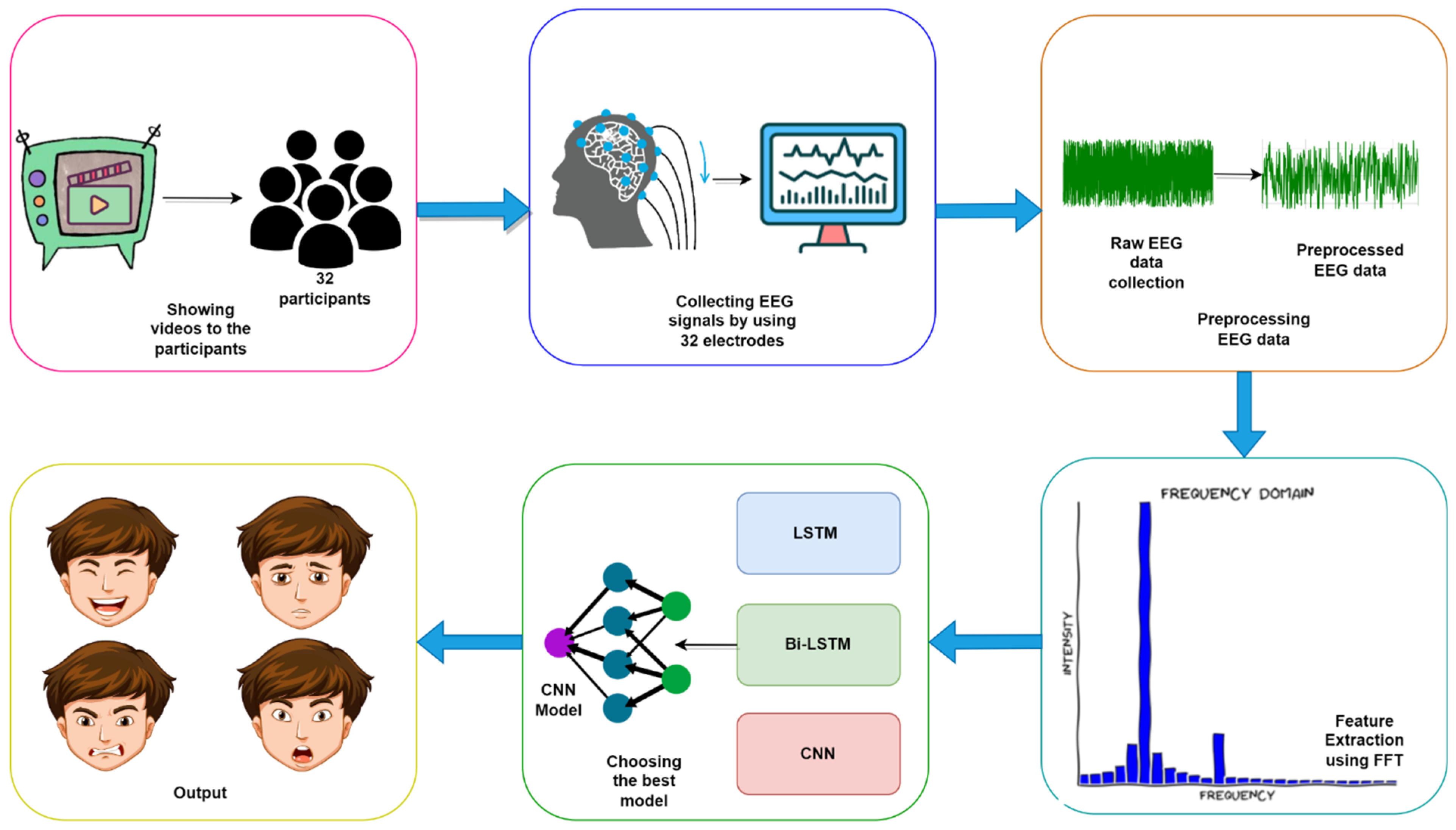
To answer research question RQ1, this experiment is conducted with multiple deep learning models. As EEG signals are time series data, LSTM and CNN can be effective for high-quality recognition. CNN [
52,
60], LSTM [
50,
51,
55], and Bi-LSTM [
55] are the most common models used with the DEAP dataset. For this reason, the LSTM, Bi-LSTM, and CNN models shown in
Table 6 are selected for recognizing emotion from brain signals. With the models established, it becomes possible for us to implement the experimental procedure and identify results.
To find out which one is more effective to recognize emotions, the raw EEG from the DEAP dataset is given as input without any kind of preprocessing or feature extraction. All three models are trained on two-class classifications of the valence and arousal labels from the DEAP dataset. To further verify the claim, these models are also trained on the binary classification of EEG data from the Confused Student dataset [
89]. The test accuracy of these models is shown in
Table 6.
In the DEAP dataset, the LSTM model achieves an average train accuracy of 87.5% and average test accuracy of 47%. The Bi-LSTM model obtains an average train accuracy of 72.5% and an average test accuracy of 31.5%. The difference between the train and test accuracy of both LSTM and Bi-LSTM is very high. It shows that both of these models have overfitting issues, as they have achieved high train accuracy while achieving low test accuracy. All of the deep learning models’ performances reported in
Table 6 are lower, as we are using the raw dataset. The raw EEG signals of the DEAP are highly complex, even for deep learning techniques. The Bi-LSTM model is very low compared to the LSTM and CNN, because Bi-LSTM attempts to learn time series data, using forward and backward passes. For most of the language data, the backward pass makes sense. However, for EEG, the backward scan does not introduce any meaningful information. As a result, the backward scan of EEG data creates a negative impact on EEG learning.
On the other hand, the 1D CNN model achieves an average train accuracy of 72.13% and average test accuracy of 63.9%. The CNN model achieves better test accuracy and handles the overfit issue much better when compared to the LSTM and Bi-LSTM models. To further verify the result, the LSTM, Bi-LSTM, and CNN models with the same number of layers are trained on another EEG dataset called the Confused Student dataset. Similar trends were observed, where the CNN model performed best with 56.65% test accuracy. LSTM and Bi-LSTM achieved 53.14% and 47.26% test accuracy, respectively.
The CNN model is selected for the remaining experiments as it outperforms LSTM and Bi-LSTM models in both EEG datasets.
4.2. Parameter Reduction
Further delving into RQ1, this particular experiment is designed to obtain a minimum parameterized model with high recognition accuracy. Because CNN performs best in recognizing emotion from brain signals, as shown in
Table 6, it is desired to find the most lightweight CNN model that would perform similarly but without losing the significant performance achieved, as shown in
Table 7.
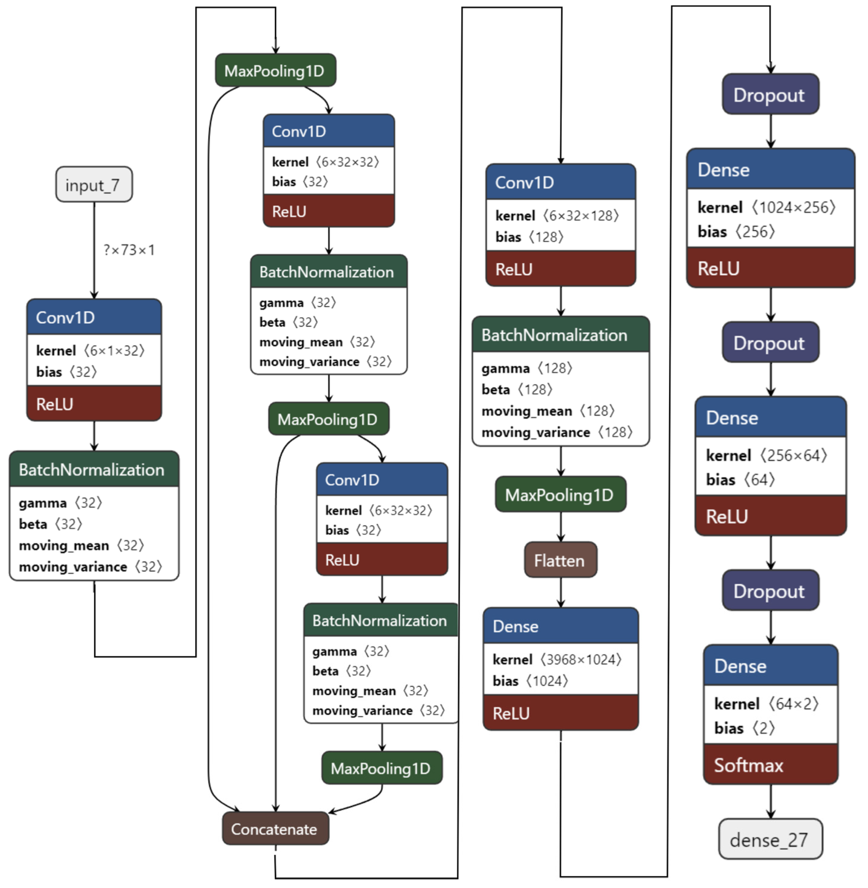
The experiment starts with the 1D CNN as shown in
Figure 7. It has four convolution layers and three dense layers. Using FFT as feature extraction, the 1D CNN model is trained on two-class classifications for the valence label.
For this experiment, the ratings of arousal, dominance, and liking are also used as feature extensions to further improve the performance of recognition as all of the four labels of the DEAP dataset are correlated. The 1D CNN model with four convolution layers and three dense layers achieved 99.89% test accuracy on the valence label after 63 epochs. However, this model is not light, since it has over 4,381,410 total parameters.
Thus, one convolution layer and one dense layer are then reduced from this to create a 1D CNN model with three convolution and two dense layers. This model is relatively lighter with a total of 70,130 parameters and it achieves 99.60% test accuracy after 30 epochs. This model is 62 times lighter than the first model in terms of the number of parameters while achieving similar performance.
Thus, one more convolution layer is reduced to achieve 99.44% testing accuracy after thirty epochs, while making the model 73 times lighter than the first model and 1.18 times lighter than the second model.
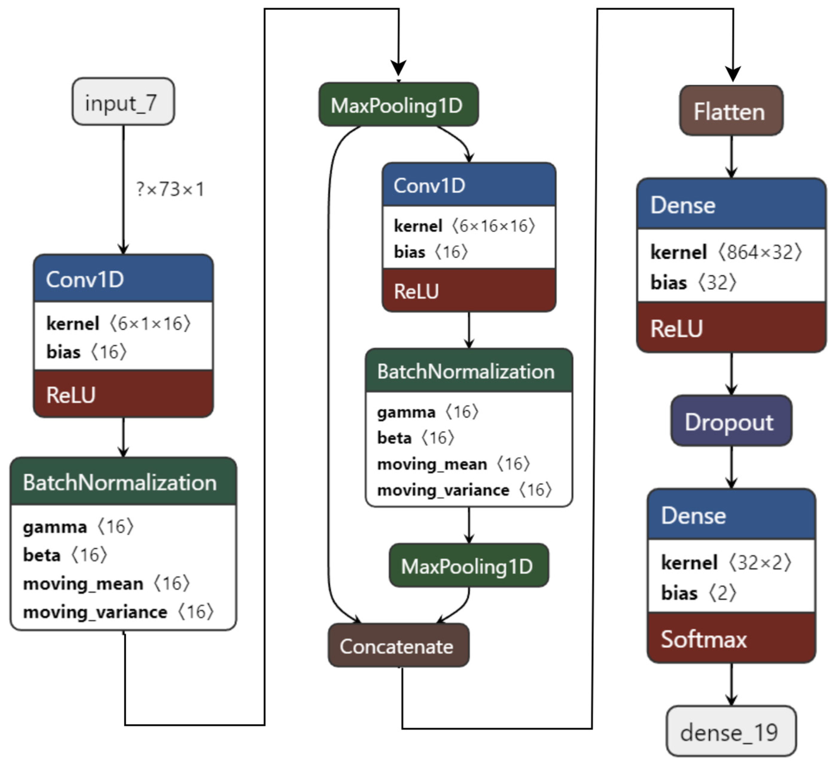
As the performance is still good, another dense layer is reduced to create a 1D CNN model with only two convolution layers and one dense layer, as shown in
Figure 8. This model has only 29,538 parameters. It is 148 times lighter than the first model, 2.37 times lighter than the second model, and twice as light as the third model. While being light, this 1D CNN model achieves 99.22% testing accuracy on the valence label for two-class classification after 100 epochs.
Next, another CNN model with 1 convolution and 2 dense layers is tested. Though this was the lightest model, with 18,706 parameters, it only achieved 96.92% testing accuracy after 30 epochs. It loses performance greatly as compared to the other models.
Among the five models referred to in
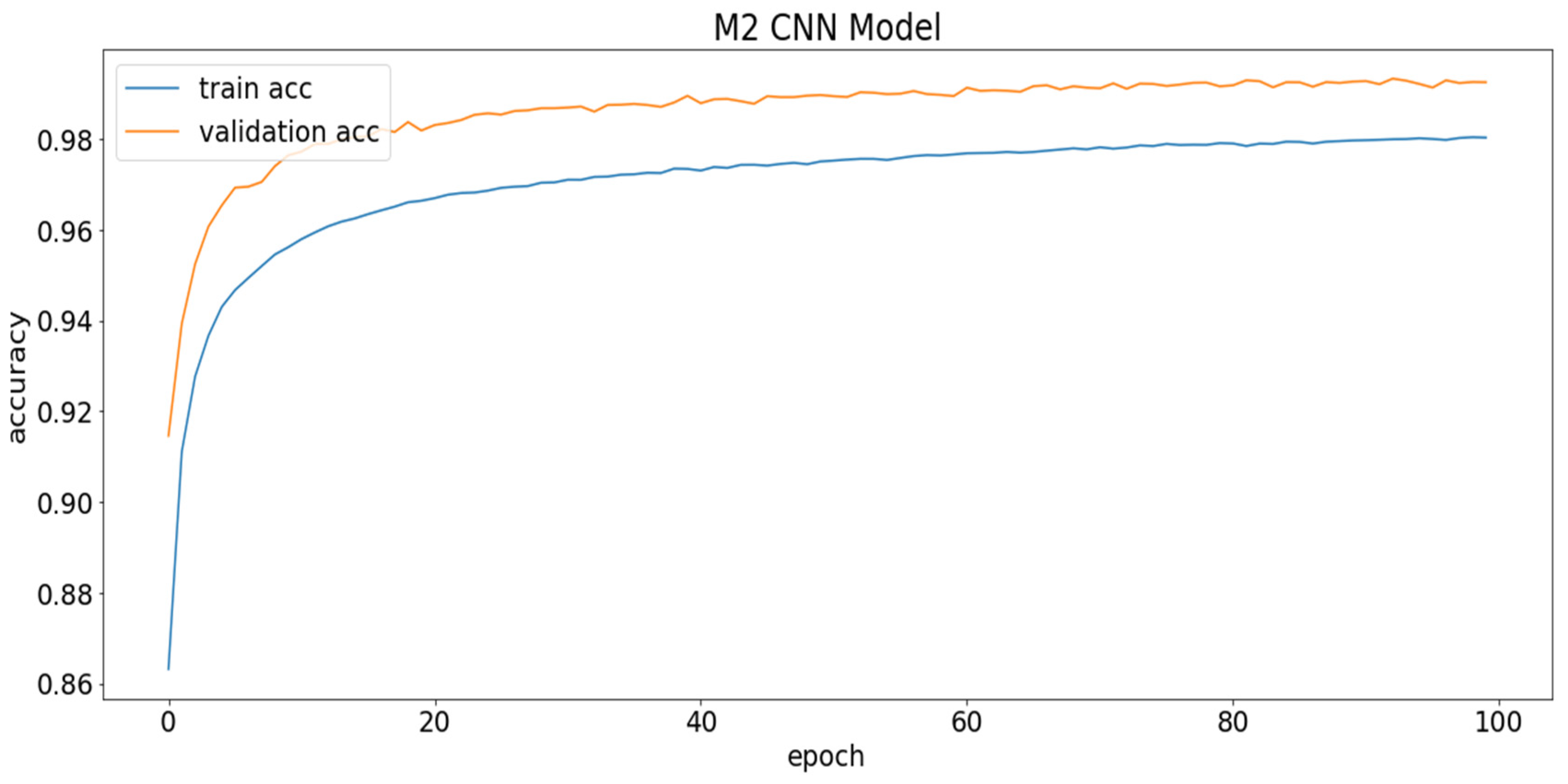
Table 7, the 1D CNN model with four convolution and three dense layers is the best in terms of testing accuracy. It is selected as the heaviest model (M1) for the remainder of the experiments since it is the heaviest model overall. On the other hand, the 1D CNN model with two convolution layers and one dense layer is selected as the light model (M2) for further experiments, as it is very light in comparison to the others, while not significantly losing performance. The validation accuracy graph of the light model is shown in
Figure 9.
To keep the model from overfitting the training data, heavy regularizers are used by adding drop-out. The curves in
Figure 9 represent how the model can generalize over the unseen test dataset. Thus, the validation accuracy is better than the training accuracy, which serves as evidence of good generalization over the unseen test data. The hyper-parameters used for these experiments are epochs = 100; batch size = 100; optimizer = Adam; loss function = categorical cross-entropy; activation function = relu (hidden layers) and soft-max (output layer).
4.3. Testing with Complementary Features
This experiment answers the research question RQ2. Two CNN models were selected (heavy and light) from the parameter reduction experiment. At this point, CNN models with and without feature extension or complementary features are tested.
In
Table 8, the results of the heavy and light 1D CNN model with feature extraction and feature extension (other ratings) are shown. The following are applicable when referring to
Table 8: M1 = heavy; M2 = light; FFT = extracted features using FFT; FE = feature extension or complementary features (other scores like dominance, liking, etc.); L = liking, D = dominance; FE-3 = three different scores (dominance, liking, arousal/valence).
While using raw EEG with the M1 model, a 61.56% and 66.25% testing accuracy was achieved for valence and arousal, respectively. However, by using FFT as feature extraction, the M1 model achieved 96.22% and 96.27% testing accuracy on valence and arousal, respectively. This is a very significant improvement over the raw EEG.
To test the effect of feature extension, liking was used as the feature extension on the M1 + FFT + FE-L experiment. This results in 98.79% and 98.6% testing accuracy for valence and arousal, respectively. Adding the dominance rating along with liking further increases the performance shown in the M1 + FFT + FE-L-D experiment. This experiment achieves 99.67% and 99.52% testing accuracy for valence and arousal, respectively.
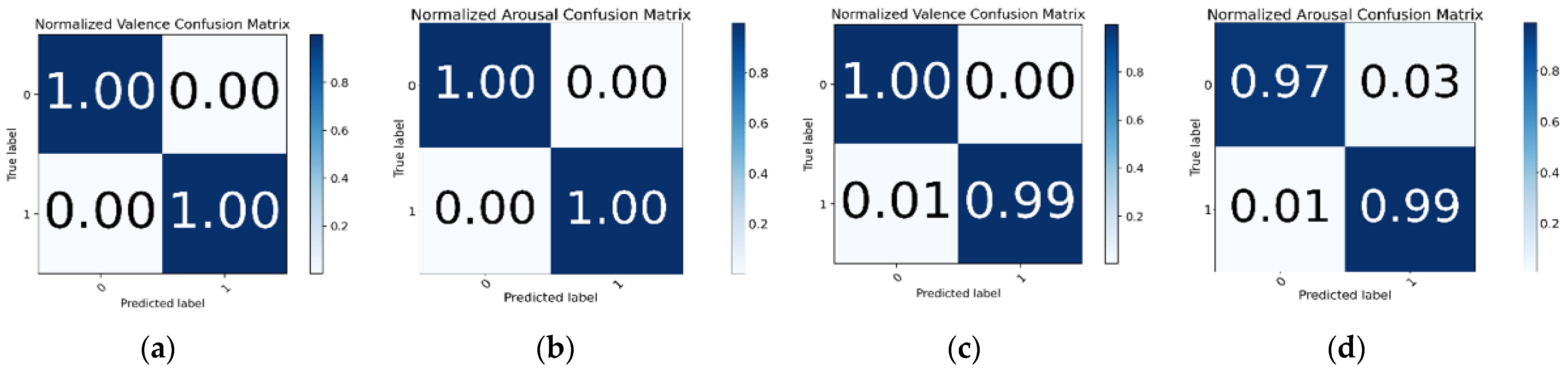
Three other ratings were added as feature extensions with respect to valence and arousal for improved accuracy. For training valence, these other three ratings (arousal, dominance, and liking) were used as feature extensions and this results in the model achieving 99.89% testing accuracy. For arousal, the M1 model was trained with FFT as feature extraction and the other three ratings (valence, arousal, and liking) as feature extension and this achieved 96.27% testing accuracy. The confusion matrix of valence and arousal for this experiment is shown in
Figure 10a,b.
The M2 model achieved 42% and 55% testing accuracy on raw EEG for valence and arousal, respectively. However, the M2 model with FFT as feature extraction achieved 78.61% and 80.22% accuracy for valence and arousal, respectively. This is a marked improvement over only the raw EEG, but as the M2 model is lightweight, its lack of feature extension becomes noticeable in its performance. In the M2 + FFT + FE-L experiment, only “liking” was used as a feature extension rating and the M2 model achieved 91.27% and 89.42% accuracy for valence and arousal, respectively. This demonstrates the importance of feature extension and how it improves the model performance significantly.
Surprisingly, in the M2 + FFT + FE-L-D experiment, using both liking and dominance ratings as a feature extension increases the M2 model’s performance for valence and arousal, which was 97.83% and 96%, respectively. This shows that adding more ratings can lead to an increase in the model’s performance.
In the M2 + FFT + FE-3 experiment, all three ratings were used, achieving 99.22% and 97.80% testing accuracy for valence and arousal, respectively. The confusion matrix for the M2 + FFT + FE-3 experiment on the valence and arousal labels is shown in
Figure 10c,d. In
Table 8, it is observed that for both M1 and M2 models, the emotion recognition performance increases significantly when applying both feature extraction (FFT) and feature extension (other ratings) together.
Accuracy is a good way to measure a model’s performance. However, accuracy alone without precision can make the model’s actual performance misleading. Accuracy can be calculated using Equation (2). When the classes are severely unbalanced, precision–recall is a helpful indicator of prediction success. Precision in information retrieval refers to how relevant the results are, whereas recall measures the number of outcomes that are relevant. Precision and recall can be calculated using Equations (3) and (4), respectively. The average value of precision and recall is the
F1 Score. Therefore, both false positives and false negatives are considered while calculating this score. The
F1 score can be calculated using Equation (5).
In
Table 9, the performance report for the M1 and M2 models is shown. The results of
Table 9 indicate that the classes are well balanced and, in all cases, the M1 model achieves almost perfect accuracy. The M2 model also performs very well.
In
Table 10, the results of previous state-of-the-art works are compared to the proposed M1 and M2 CNN models of this experiment. To obtain these results, FFT-produced frequencies, dominance, and liking ratings were used as features. We report the test accuracy of the valance and arousal classes and the average accuracy of these two labels to compare them with the previous results. Hasan et al. [
48] used a 1D CNN model with four convolution layers and three dense layers, which may be considered a heavy model. They also used FFT as a feature extraction technique to achieve 96.63% and 96.17% test accuracy on valence and arousal, respectively, for two-class classification. On the other hand, the proposed light M2 model with only the two convolutions and one dense layer outperforms their accuracy on both valence and arousal labels. The proposed M1 model exceeds their accuracy by an even greater margin.
As shown in
Table 10, Yin et al. [
47] used a fusion of graph convolution neural network, LSTM, and differential entropy as feature extraction techniques, achieving only 90.45% and 90.60% test accuracy on valence and arousal, respectively. Both of the proposed M1 and M2 models exceed their accuracy by 8–9%. In the following row of
Table 10, Ma et al. [
60] used multi-modal residual LSTM network without any feature extraction technique and only achieved 92.30% and 92.87% accuracy for valence and arousal, respectively. The proposed M1 and M2 models outperform their model by 7%. Next, Alhalaseh et al. [
54] used a CNN model and two feature extraction techniques called entropy and Higuchi’s fractal dimension (HFD). They achieved 95.2% testing accuracy on two-class classification. The proposed light and heavy 1D CNN exceeds their accuracy by 4%. On the next line, Cui et al. [
46] achieved 94.02% and 94.86% test accuracy on valence and arousal, respectively, by fusing both CNN and BiLSTM. Their modeling technique is called DE-CNN-BiLSTM and they used differential entropy as a feature extraction technique. Their fusion of CNN and BiLSTM definitely made their model heavy. However, despite using a particularly heavy model, their accuracy falls behind by 5% compared to both of the proposed M1 and M2 models.
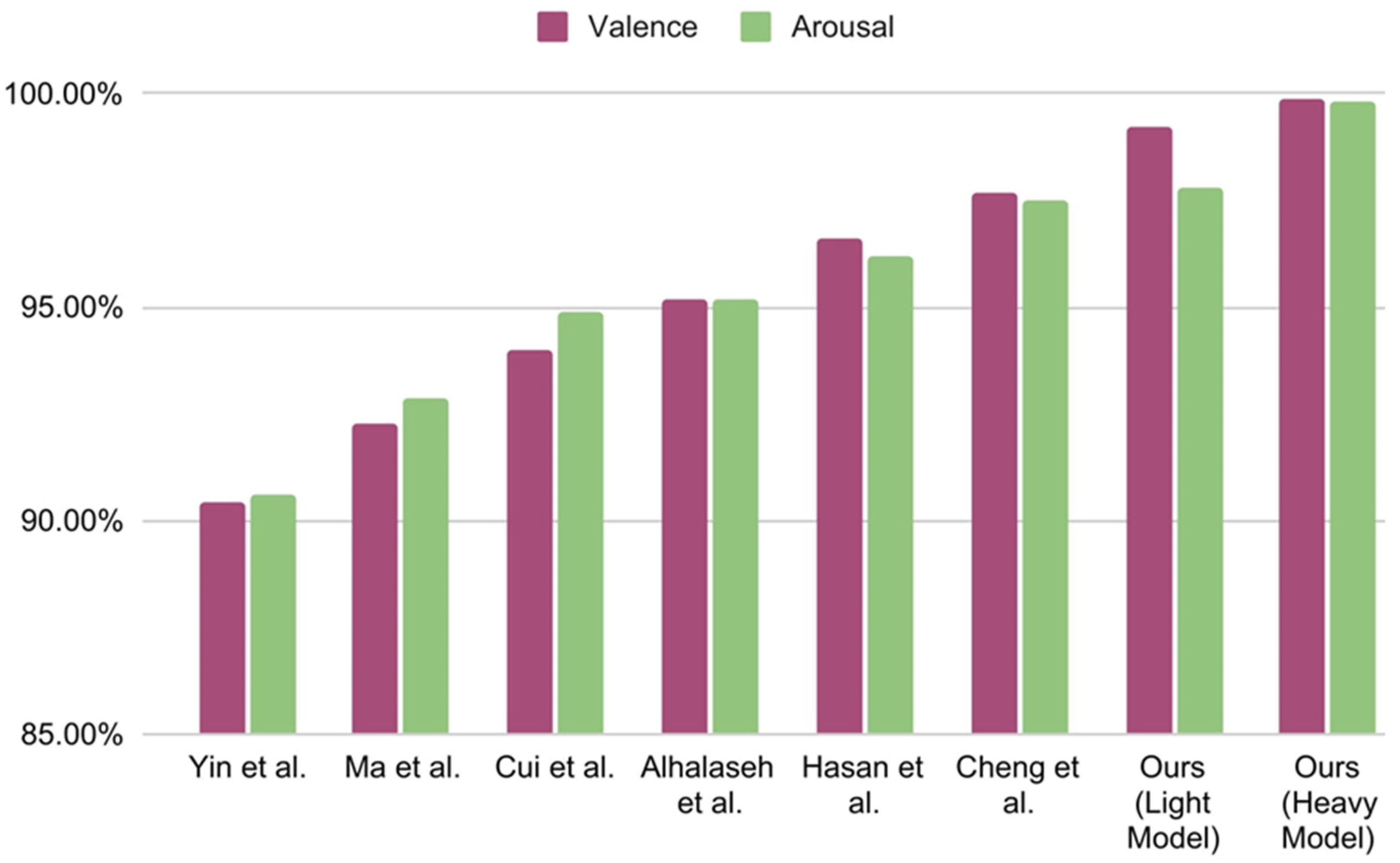
In the current study, both of the proposed CNN models use a residual connection, and the features are extracted using FFT, while the other ratings are used as feature extensions. The result, shown in
Table 10 compared with the other aforementioned models, is plotted in
Figure 11 for visualizing the result. The proposed 1D CNN model with two convolution layers and one dense layer (the light model) achieves 99.22% and 97.80% test accuracy on valence and arousal, respectively, for binary classification. On the other hand, the 1D CNN model with four convolution layers and three dense layers (heavy model) achieve 99.89% and 99.83% testing accuracy on valence and arousal, respectively. This accuracy is highest even when compared to the other state-of-the-art works shown in
Table 10.
4.4. The Effective EEG Length
In this section, we explain the solution for research question RQ3. Hasan et al. [
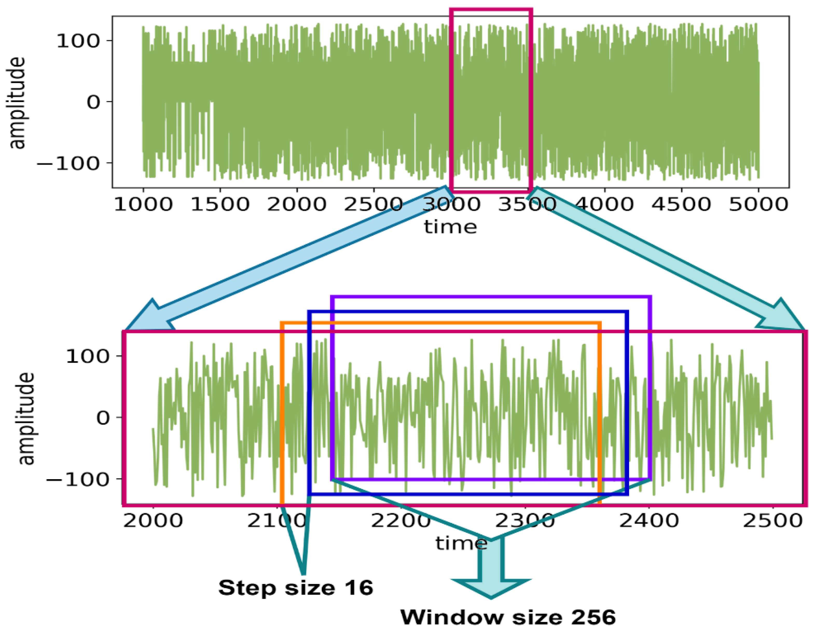
48] used an EEG length of 2 s (window size 256) and got 96.18% accuracy for arousal and 96.63% accuracy for valence. In this paper, all the previous experiments have been conducted using a 256-window size, corresponding to a two-second time slice of EEG data. However, to recognize emotion from brain signals in real-time, it becomes necessary to reduce the EEG length as much as possible.
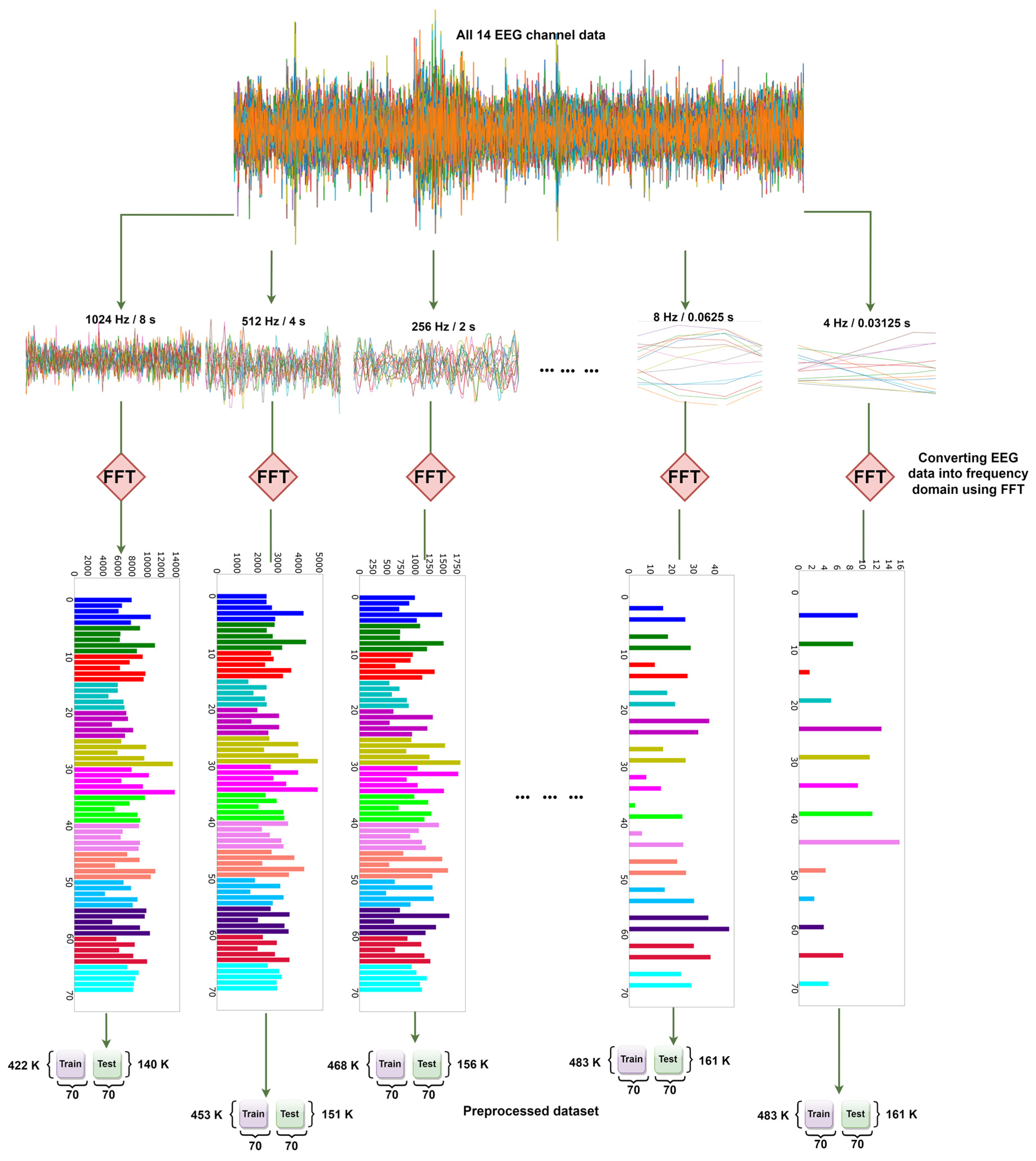
To experiment with the effects of the window size of FFT on the accuracy, multiple preprocessed files are generated by varying window sizes ranging from 4 to 1024. The process of generating these is shown in
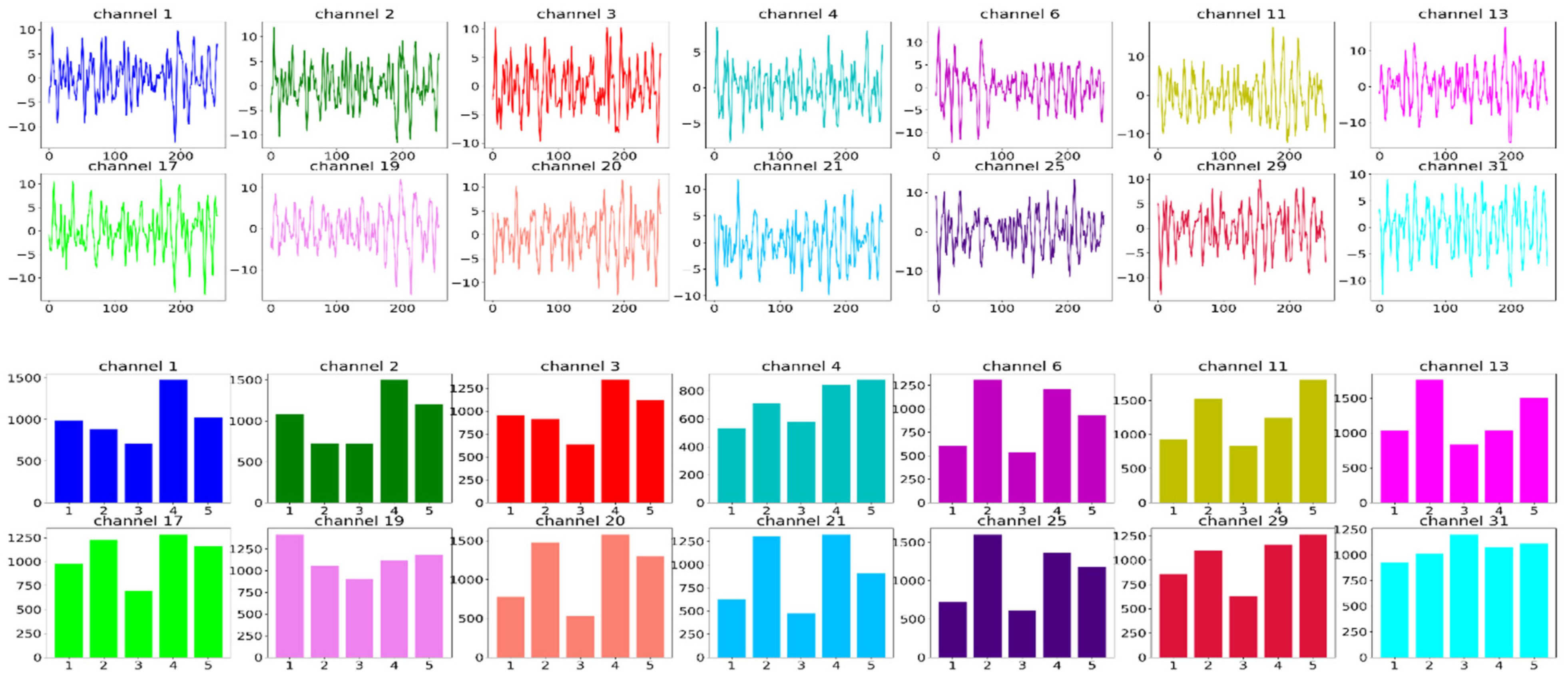
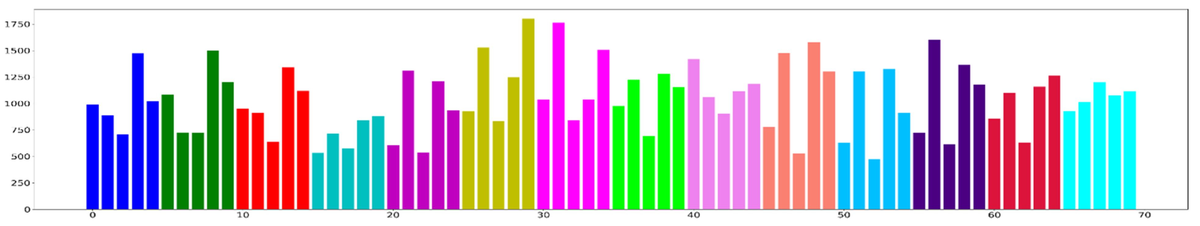
Figure 12. First, EEG data with 14 channels are selected, with different window sizes subsequently taken each time. Then, after applying FFT, the preprocessed dataset is ultimately created for that particular window size or time slice.
In
Table 11, FFT is used for feature extraction with different window sizes. This is done to test the accuracy of various time slices on DEAP EEG data. As the M1 model achieves better accuracy than the M2 in each of the previous experiments, these experiments are therefore tested using the M2 model (two convolutions + one dense). This is because, if M2 can perform with an accuracy of more than 90%, then M1 will be able to exceed that level of accuracy. Hence, the lighter model is tested, rather than the heavier M1 model, to make the experiment more challenging and reliable. In the DEAP dataset, the sample rate is 128 Hz; thus, using the 128-window size can be considered equal to one second. The window size is changed from 4 to 1024 to conduct the experiments.
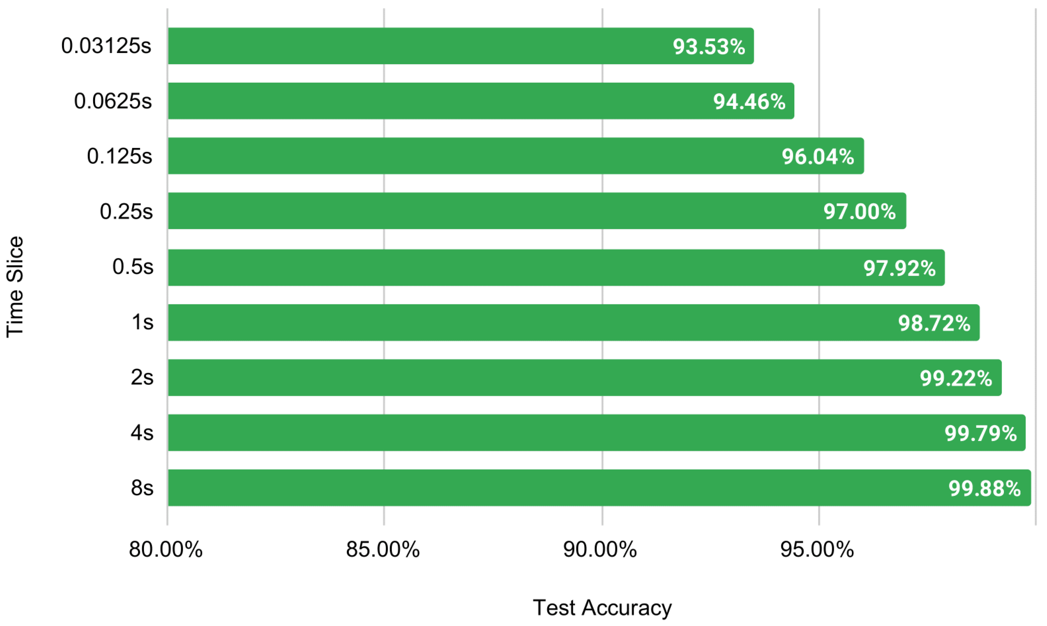
To visualize the results clearly, a bar plot is shown in
Figure 13. The time slice is directly proportional to the testing accuracy. The light model with two convolutions and one dense layer achieves a respectable 93.53% accuracy with a 0.03-s time slice of EEG data. It shows the possibility of using EEG data to recognize emotions in real-time. For the rest of the experiments, a window size of 256, or two-second time slice, is selected as it provides a balance between lower time slices without losing accuracy significantly.
4.5. Training Size Requirement
Finally, solutions for RQ4 are explored in this experiment. Though the proposed models achieved state-of-the-art accuracy, it is possible that using a higher training size may affect the model’s performance. Hence, it is important to understand how effectively the model will perform with different training sizes.
Thus, as shown in
Table 12, a different combination of the train–test split set was tested. Each of the experiments was executed in Google Colab using the M2 model for 100 epochs. The required training and testing time is noted for each split. Wall time is the amount of time that a wall clock (or a stopwatch held in the hand) would indicate has passed between the beginning and end of the process. The amount of time spent in user code and the amount of time spent in kernel code are referred to as user-CPU time and system-CPU time, respectively. Among the options available for the train–test split, a 75/25 split attained the best test accuracy of 99.26%.
Google Colab Pro Configuration:
In
Table 13, the test accuracy of the M2-CNN model is compared with that of Alhalaseh et al. [
54] for different training dataset size splits. Alhalaseh et al. [
54] used CNN, K-Nearest Neighbour (KNN), Naïve Bayes (NB), and Decision tree (DT). The common train/test splits between both of the studies were 80/20 and 50/50. In both cases, this paper’s M2-CNN model outperforms the previous study by a sizable margin.
Based on these experiments, all of the stated research questions are restated below and are now answered empirically.
RQ1: Which deep learning model is more effective for EEG as a form of time series signal recognition?
Among CNN, LSTM, and Bi-LSTM deep learning models, CNN performs the best on the raw EEG signals. The M1 CNN model contains 4381 K parameters, while the M2 model has only 29.5 K parameters, with similar recognition accuracy.
Table 6 and
Table 7 represent the corresponding experiment results.
RQ2: Can feature extraction improve the recognition accuracy of a deep learning model? What is the most effective feature set?
Features extracted by FFT can boost recognition accuracy of CNN by at least 30% (raw EEG accuracy 66% and FFT feature-based model accuracy 96%). The most effective feature set is a combination of frequency domain features extracted by FFT, with deep features extracted by Conv layers of CNN, and complementary features using additional information such as dominance and liking.
Table 8 represents the corresponding experiment results.
RQ3: What is the minimum EEG signal required for good recognition? Can it be done in real-time?
Only two seconds of EEG signal are required to attain over 99% accuracy. Even 125 milliseconds of EEG data can achieve more than 96% accuracy for valence.
Table 11 and
Figure 13 represent the corresponding results.
RQ4: How much data and time are required for training the model to achieve a reasonable performance?
Only 50% of the EEG dataset can achieve over 99% accuracy on valence, and only 10% of the dataset can achieve a valence accuracy of 96.84%. The model training time with 100 epochs is approximately 1 h (50% dataset), while the model can predict 176 K data points in under 40 s.
Table 12 and
Table 13 represent the corresponding results.


 ,
, 


