
Ultrasonic Testing of Mechanical Changes in a Water-Filled Pipe with Multi-Mode and Broadband Signals and Two-Level Compensation
Abstract
:1. Introduction
2. Theory
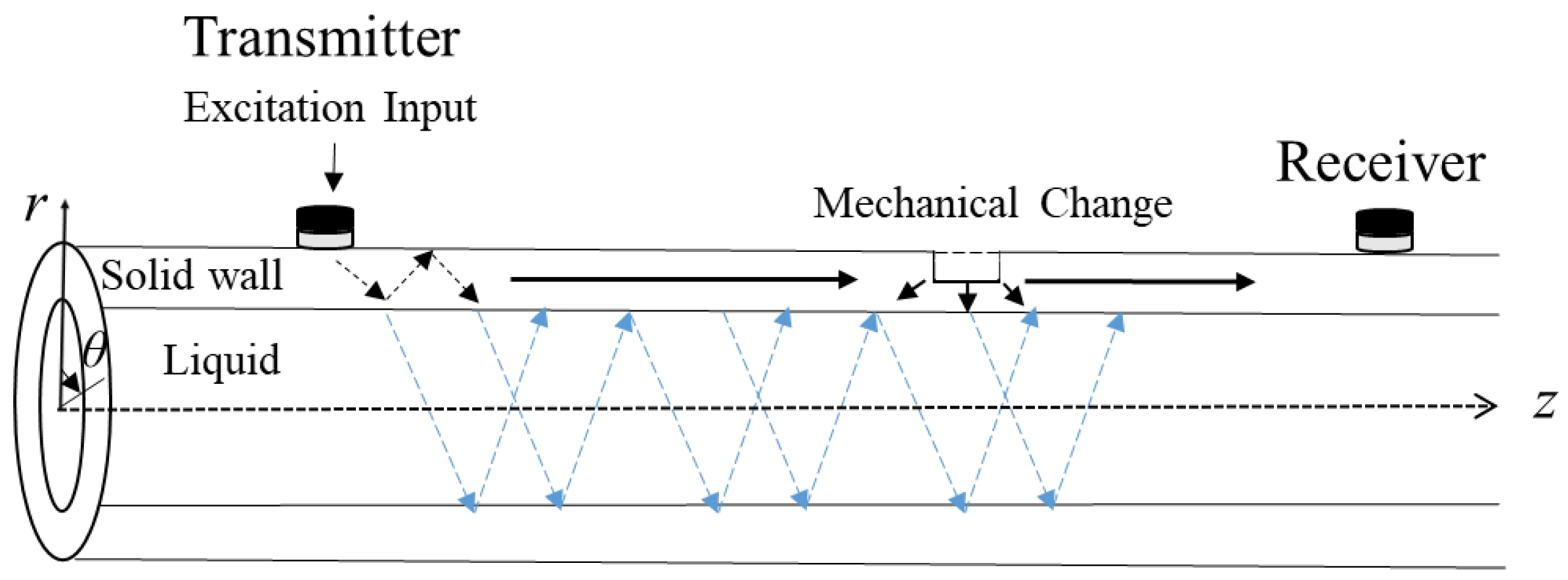
2.1. Multi-Mode Ultrasonic Signals by Non-Axisymmetric Partial Loading
2.2. Baseline and Monitoring Ultrasonic Signals
2.3. 1st EOC Compensation Method
2.4. 2nd EOC Compensation Method
3. Experimental Setup
4. Estimation of Mechanical Changes in the Presence of EOC Changes
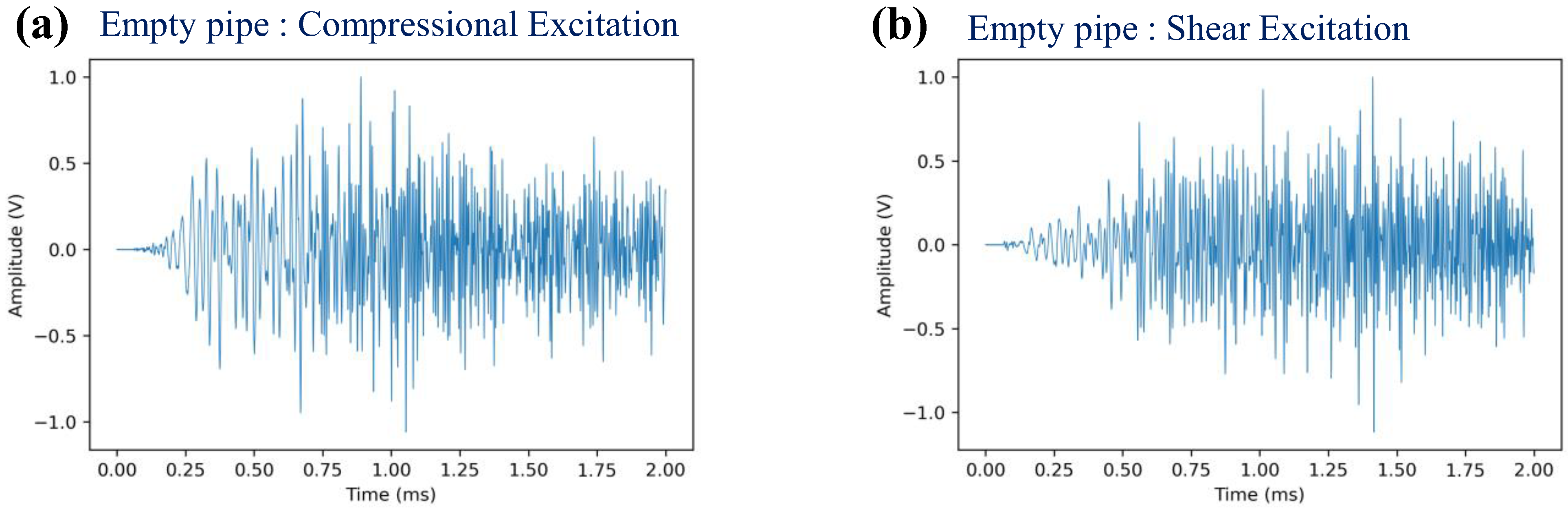
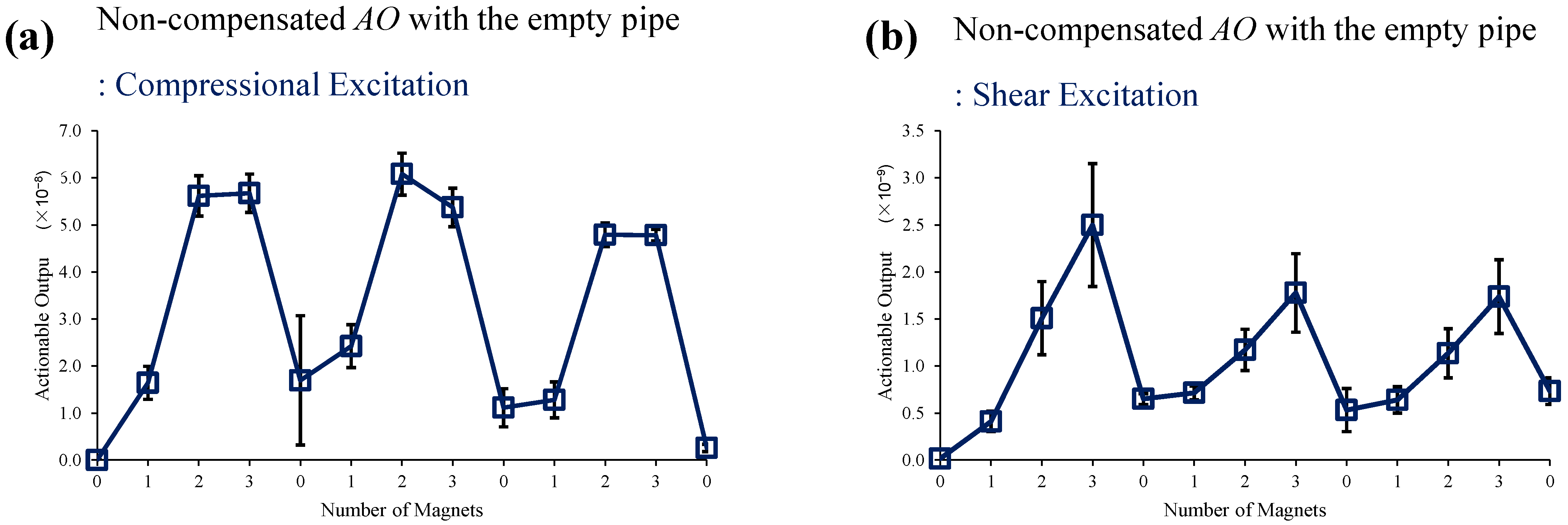
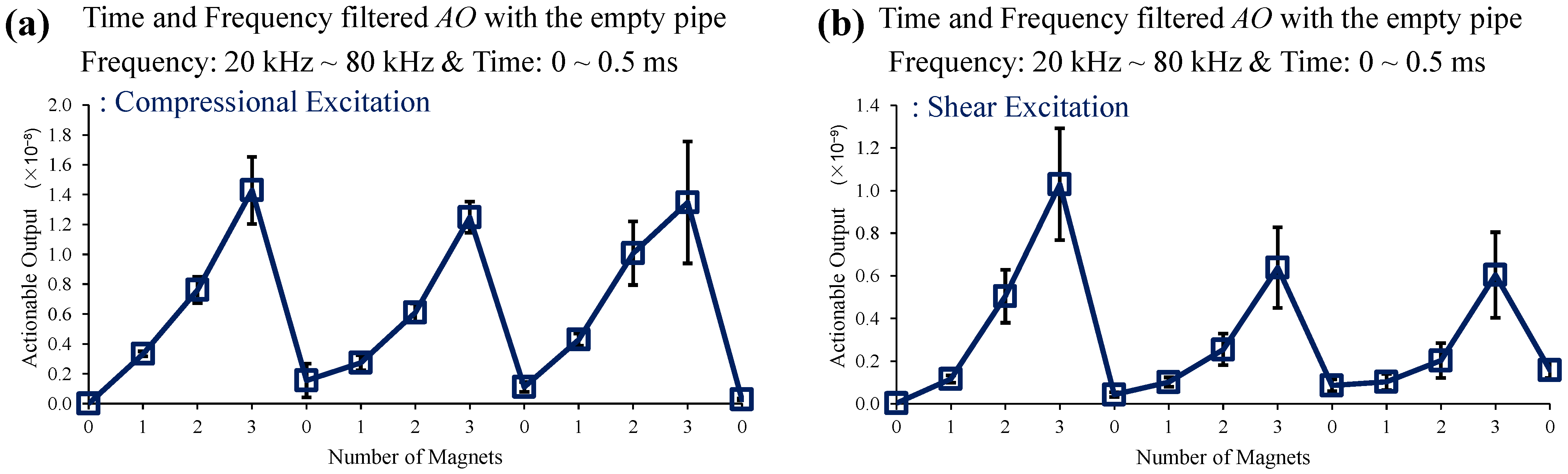
4.1. Empty Pipe
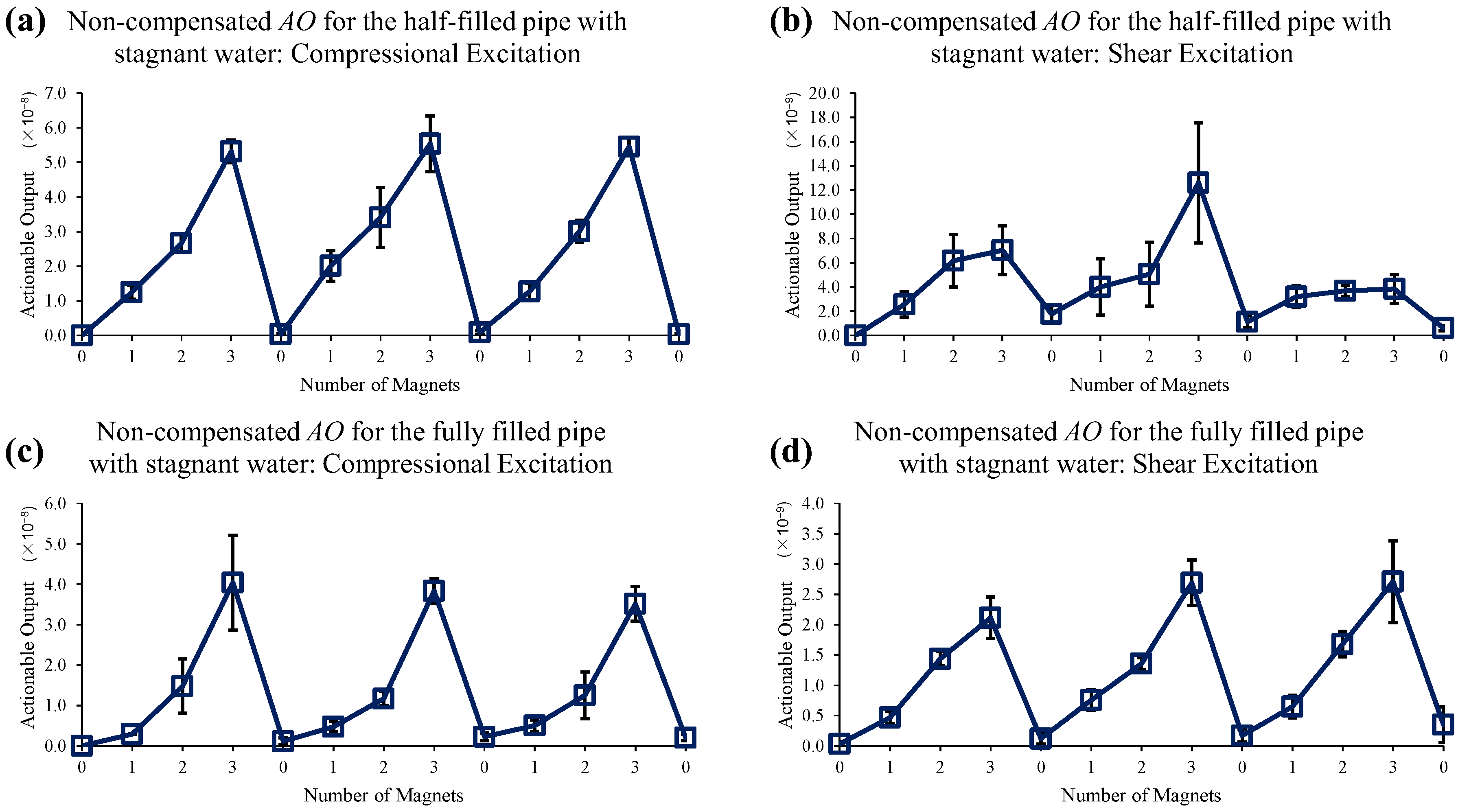
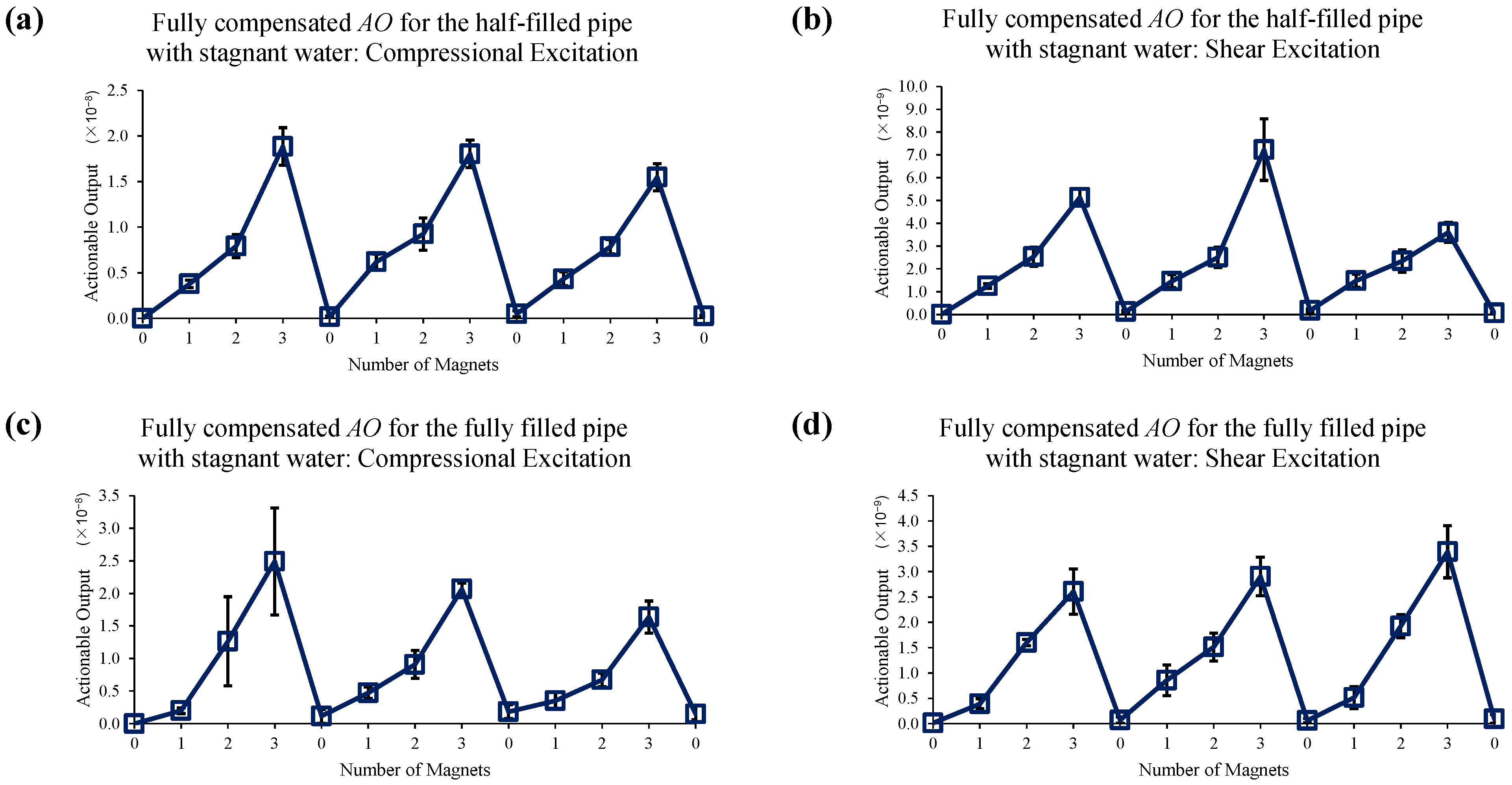
4.2. Stagnant Water
4.3. Water Flow
5. Summary and Conclusions
Author Contributions
Funding
Institutional Review Board Statement
Informed Consent Statement
Data Availability Statement
Acknowledgments
Conflicts of Interest
References
- Yibo, L.; Liying, S.; Zhidong, S.; Yuankai, Z. Study on energy attenuation of ultrasonic guided waves going through girth welds. Ultrasonics 2006, 44, e1111–e1116. [Google Scholar] [CrossRef] [PubMed]
- Barbian, A.; Beller, M. In-Line Inspection of High Pressure Transmission Pipelines: State-of-the-Art and Future Trends. In Proceedings of the 18th World Conference on Nondestructive Testing, Durban, South Africa, 16–20 April 2012. [Google Scholar]
- Zhao, X.; Rose, J.L. Guided circumferential shear horizontal waves in an isotropic hollow cylinder. J. Acoust. Soc. Am. 2004, 115, 1912–1916. [Google Scholar] [CrossRef]
- Cawley, P.; Cegla, F.; Galvagni, A. Guided waves for NDT and permanently-installed monitoring. Insight-Non-Destr. Test. Cond. Monit. 2012, 54, 594–601. [Google Scholar] [CrossRef]
- Galvagni, A.; Cawley, P. Permanently installed guided wave pipeline monitoring. In Proceedings of the AIP Conference Proceedings, Denver, CO, USA, 15–20 July 2012; pp. 159–166. [Google Scholar] [CrossRef]
- Lee, P.-H.; Yang, S.-K. Defect Inspection of Complex Structure in Pipes by Guided Waves. In IUTAM Symposium on Recent Advances of Acoustic Waves in Solids; Springer: Dordrecht, The Netherlands, 2010; pp. 389–395. [Google Scholar] [CrossRef]
- Belanger, P.; Cawley, P. Feasibility of low frequency straight-ray guided wave tomography. NDT E Int. 2009, 42, 113–119. [Google Scholar] [CrossRef]
- Vinogradov, S.A. Magnetostrictive transducer for torsional guided waves in pipes and plates. Mater. Eval. 2009, 67, 333–341. [Google Scholar]
- Løvstad, A.; Cawley, P. The reflection of the fundamental torsional guided wave from multiple circular holes in pipes. NDT E Int. 2011, 44, 553–562. [Google Scholar] [CrossRef]
- Mariani, S.; Heinlein, S.; Cawley, P. Location specific temperature compensation of guided wave signals in structural health monitoring. IEEE Trans. Ultrason. Ferroelectr. Freq. Control 2019, 67, 146–157. [Google Scholar] [CrossRef] [PubMed] [Green Version]
- Torres-Arredondo, M.; Fritzen, C.P. Ultrasonic guided wave dispersive characteristics in composite structures under variable temperature and operational conditions. In Proceedings of the 6th European Workshop in Structural Health Monitoring, EWSHM, Dresden, Germany, 3–6 July 2012; pp. 261–268. [Google Scholar]
- Kwun, H.; Bartels, K.A.; Dynes, C. Dispersion of longitudinal waves propagating in liquid-filled cylindrical shells. J. Acoust. Soc. Am. 1999, 105, 2601–2611. [Google Scholar] [CrossRef]
- Nagamizo, H.; Kawashima, K.; Miyauchi, J. NDE of pipe inner corrosion with delayed echoes of SV wave propagated circumferentially in liquid-filled pipes. In Proceedings of the ASME Pressure Vessels and Piping Conference, Cleveland, OH, USA, 20–24 July 2003; Volume 16974, pp. 7–12. [Google Scholar]
- Perfetto, D.; Khodaei, Z.S.; De Luca, A.; Aliabadi, M.H.; Caputo, F. Experiments and modelling of ultrasonic waves in composite plates under varying temperature. Ultrasonics 2022, 126, 106820. [Google Scholar] [CrossRef] [PubMed]
- Giannakeas, I.N.; Sharif Khodaei, Z.; Aliabadi, M.H. An up-scaling temperature compensation framework for guided wave–based structural health monitoring in large composite structures. Struct. Health Monit. 2022, 1–22. [Google Scholar] [CrossRef]
- Perfetto, D.; Lamanna, G.; Petrone, G.; De Fenza, A.; De Luca, A. A modelling technique to investigate the effects of quasi-static loads on guided-wave based structural health monitoring systems. Forces Mech. 2022, 9, 100125. [Google Scholar] [CrossRef]
- Yu, J.G.; Zhang, B.; Elmaimouni, L.; Zhang, X.M. Guided waves in layered cylindrical structures with sectorial cross-section under axial initial stress. Mech. Adv. Mater. Struct. 2021, 28, 457–466. [Google Scholar] [CrossRef]
- Ju, T.; Findikoglu, A.T. Monitoring of corrosion effects in pipes with multi-mode acoustic signals. Appl. Acoust. 2021, 178, 107948. [Google Scholar] [CrossRef]
- Li, J.; Rose, J.L. Excitation and propagation of non-axisymmetric guided waves in a hollow cylinder. J. Acoust. Soc. Am. 2001, 109, 457–464. [Google Scholar] [CrossRef] [PubMed]
- Rose, J.L. Ultrasonic Guided Waves in Solid Media; Cambridge University Press: Cambridge, UK, 2014; ISBN 1107048958. [Google Scholar]
- Ju, T.; Findikoglu, A.T. Monitoring of mechanical changes in a pipe assembly with complex geometry using multi-mode acoustic signals. Appl. Acoust. 2022, 192, 108749. [Google Scholar] [CrossRef]
- Nawab, S.H. Short-time Fourier transform. Adv. Top. Signal Process. 1987, 289–337. [Google Scholar] [CrossRef]


Publisher’s Note: MDPI stays neutral with regard to jurisdictional claims in published maps and institutional affiliations. |
© 2022 by the authors. Licensee MDPI, Basel, Switzerland. This article is an open access article distributed under the terms and conditions of the Creative Commons Attribution (CC BY) license (https://creativecommons.org/licenses/by/4.0/).
Share and Cite
Ju, T.; Findikoglu, A.T. Ultrasonic Testing of Mechanical Changes in a Water-Filled Pipe with Multi-Mode and Broadband Signals and Two-Level Compensation. Sensors 2022, 22, 8647. https://doi.org/10.3390/s22228647
Ju T, Findikoglu AT. Ultrasonic Testing of Mechanical Changes in a Water-Filled Pipe with Multi-Mode and Broadband Signals and Two-Level Compensation. Sensors. 2022; 22(22):8647. https://doi.org/10.3390/s22228647
Chicago/Turabian StyleJu, Taeho, and Alp T. Findikoglu. 2022. "Ultrasonic Testing of Mechanical Changes in a Water-Filled Pipe with Multi-Mode and Broadband Signals and Two-Level Compensation" Sensors 22, no. 22: 8647. https://doi.org/10.3390/s22228647