
Pavement Distress Estimation via Signal on Graph Processing

 , , and
Abstract
:1. Introduction
1.1. Background
1.2. Objectives of the Current Work and Problem Statement
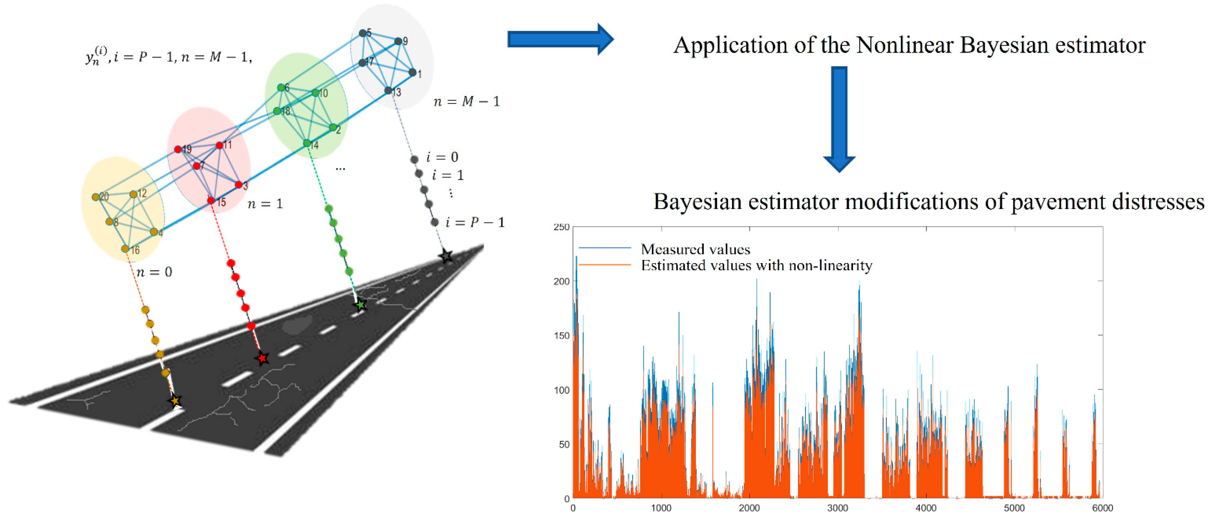
- We introduce a novel signal on graph model of the observed distress metrics; specifically, we consider the distress metrics acquired at different spatial sections as signal values associated with the vertices of a graph. The graph edges represent (i) the correlation among different distress metrics at a given spatial section and (ii) the correlation among spatially adjacent measurements of the same metric.
- We derive a novel optimal estimator of the distress metrics. The novel nonlinear Bayesian estimator is built on top of a recent model for signal defined on graphs [42], and it is optimal in the sense that it minimizes the mean square estimation error. In pavement engineering, the Bayesian analysis can be used to obtain and update the values of parameters based on the historical data and to provide a posterior probability distribution for the parameters [43].
2. Measurement and Evaluation of Pavement Conditions
- Alligator cracking occurs in areas subjected to repeated traffic loads. It originates at the bottom of the hot mix asphalt (HMA) layers, where the tensile stress–strain induced by loads is highest. The cracks propagate on to the surface in parallel ways at first, then interconnect to form polyhedral signs at acute angles, smaller than 60 cm on the longest side;
- Rutting is a road surface depression or groove due to the travel of wheels or skis. The deformation of the asphalt concrete pavement or subbase material can cause the ruts, which can become unsafe during rainy events, when the paths are filled with water;
- Longitudinal and transverse cracking happens lengthwise or crosswise at approximately right angles to the pavement’s centerline or laydown direction. These types of cracks are not usually load-associated but can occur, for example, at low temperature or because of asphalt hardening. Nonfilled crack widths less than 6 mm for airport pavement and 10 mm for road pavement are always considered of low severity.
- Block cracks divide the pavement surface into rectangular pieces whose extensions generally range between 0.1 m2 and 10 m2. They are caused by the shrinkage of the asphalt concrete due to the cyclical variation of daily temperature. Whatever is the load phenomenon, the asphalt manifests an excessive hardening, and so it can occur on non-trafficked sections;
- Raveling is due to the wearing away of the pavement surface with the loss of bituminous material and the consequent dislodging of the aggregate materials. The phenomenon indicates poor quality of the mixture and a hardening of the asphalt binder.
- Lane/shoulder drop-off is the difference in elevation between the traffic lane and the shoulder. Generally, the shoulder settles because of the consolidation or pumping of the underlying material.
- Potholes are bowl-shaped depressions with a diameter less than 1 m on the road surface. The edges are generally sharp, and the sides are vertical. They are formed when small portions of pavement are removed by traffic, and the phenomenon is accelerated by the presence of water that can stagnate inside them.
3. Proposed Model of Road Distress Estimation as a Signal on Graph
4. Nonlinear Bayesian Estimation of the Road Distress
4.1. Performance of the Bayesian Estimator for the Toy Case
5. Application of the Proposed Model to Real Data
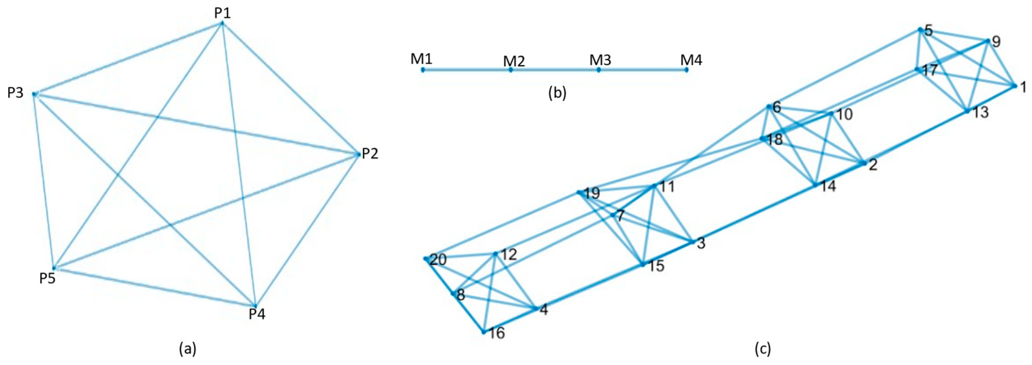
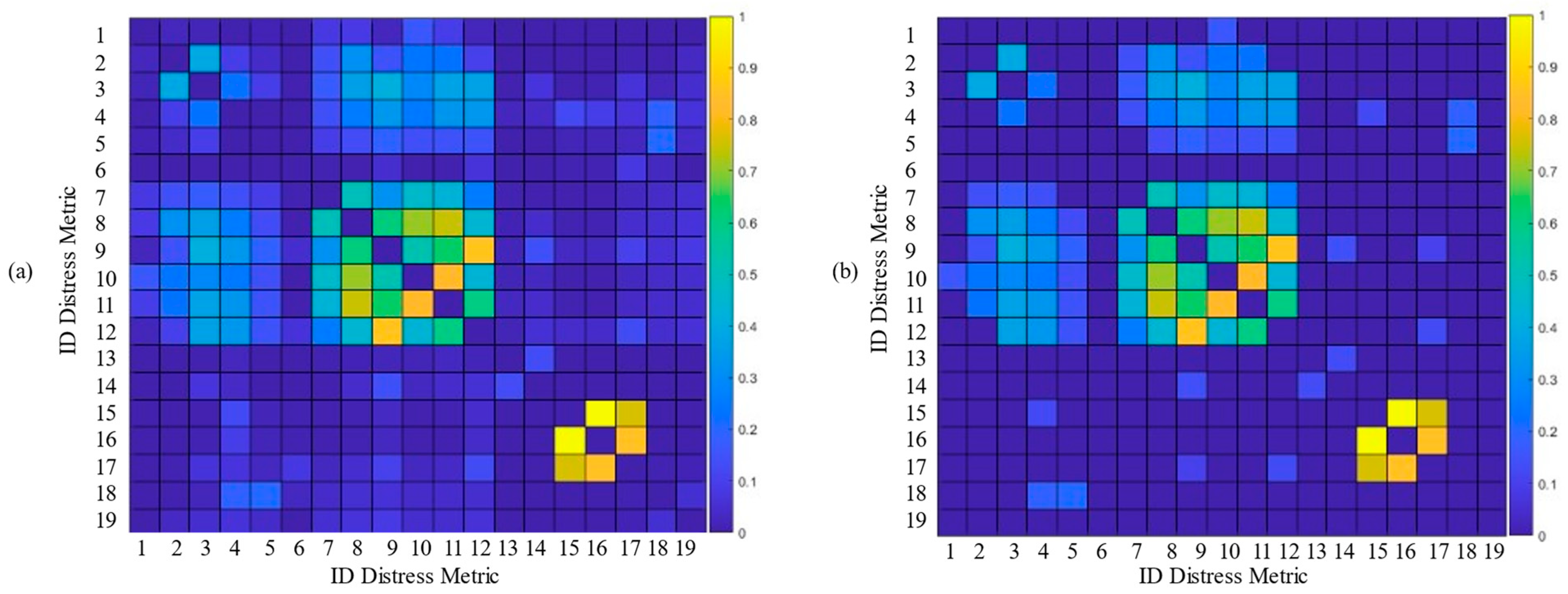
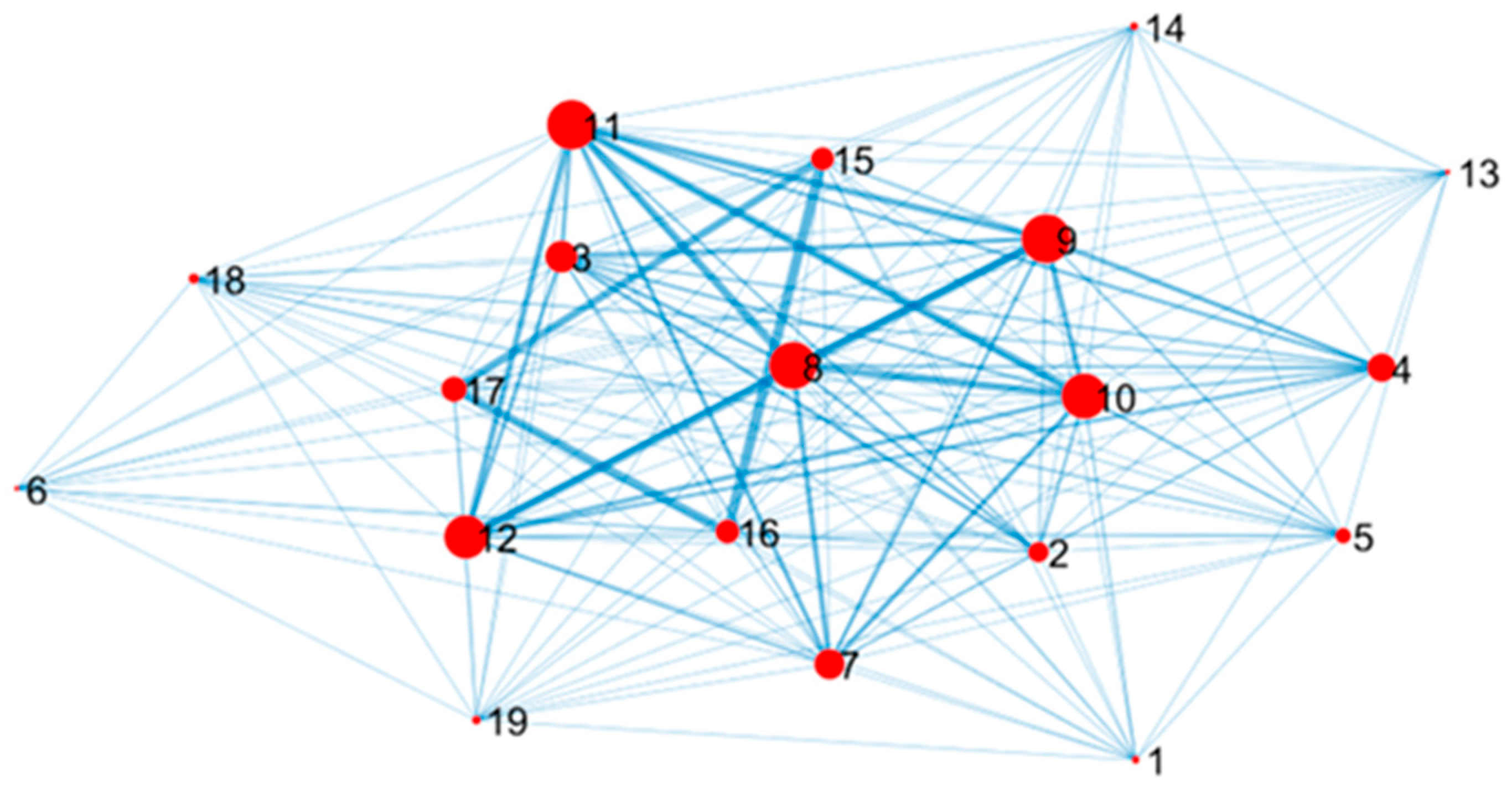
5.1. Construction of the Graph of the Metrics
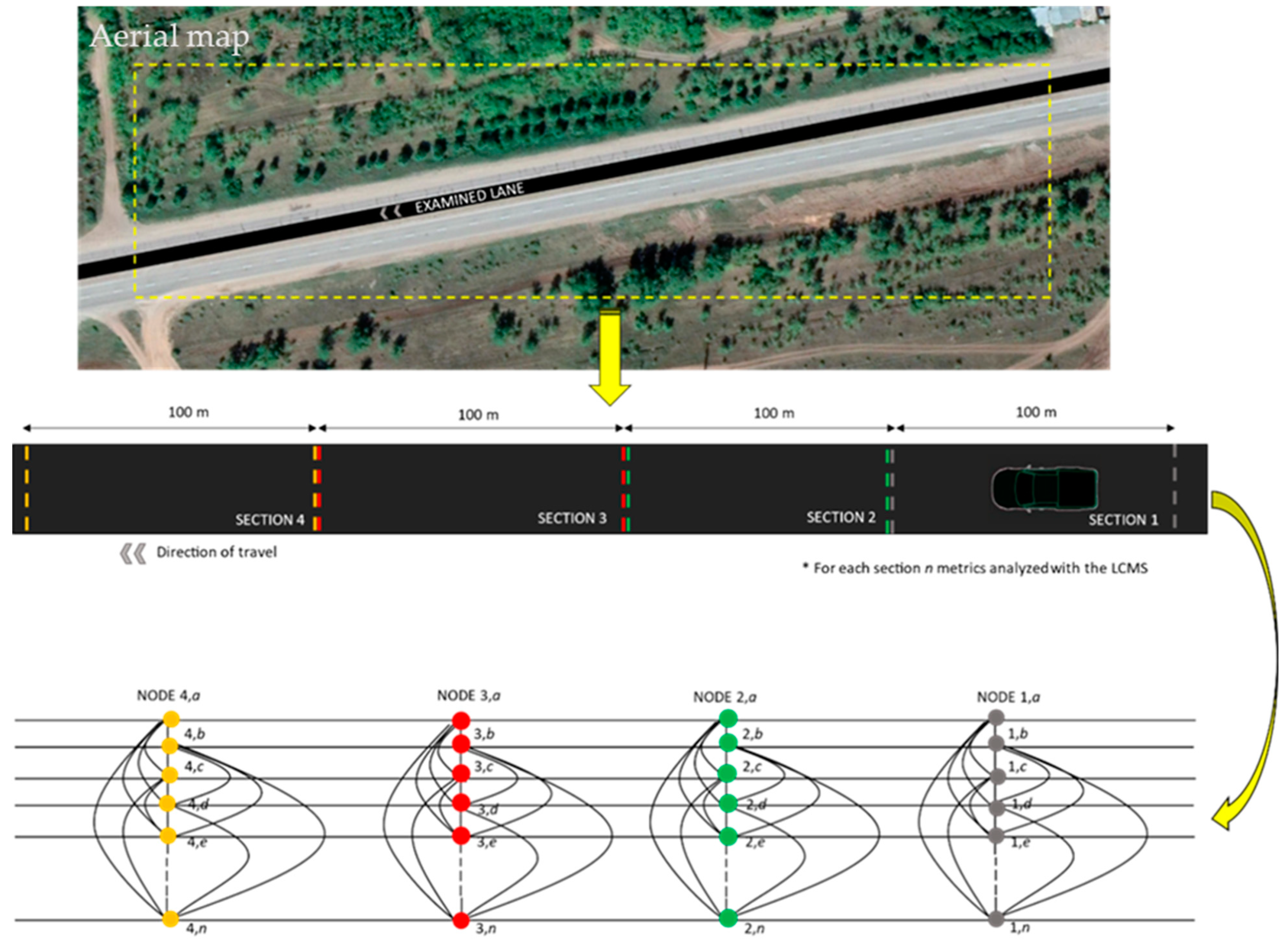
5.2. Construction of the Path Graph on Adjacent Spatial Sections
6. Experimental Results
7. Conclusions and Future Works
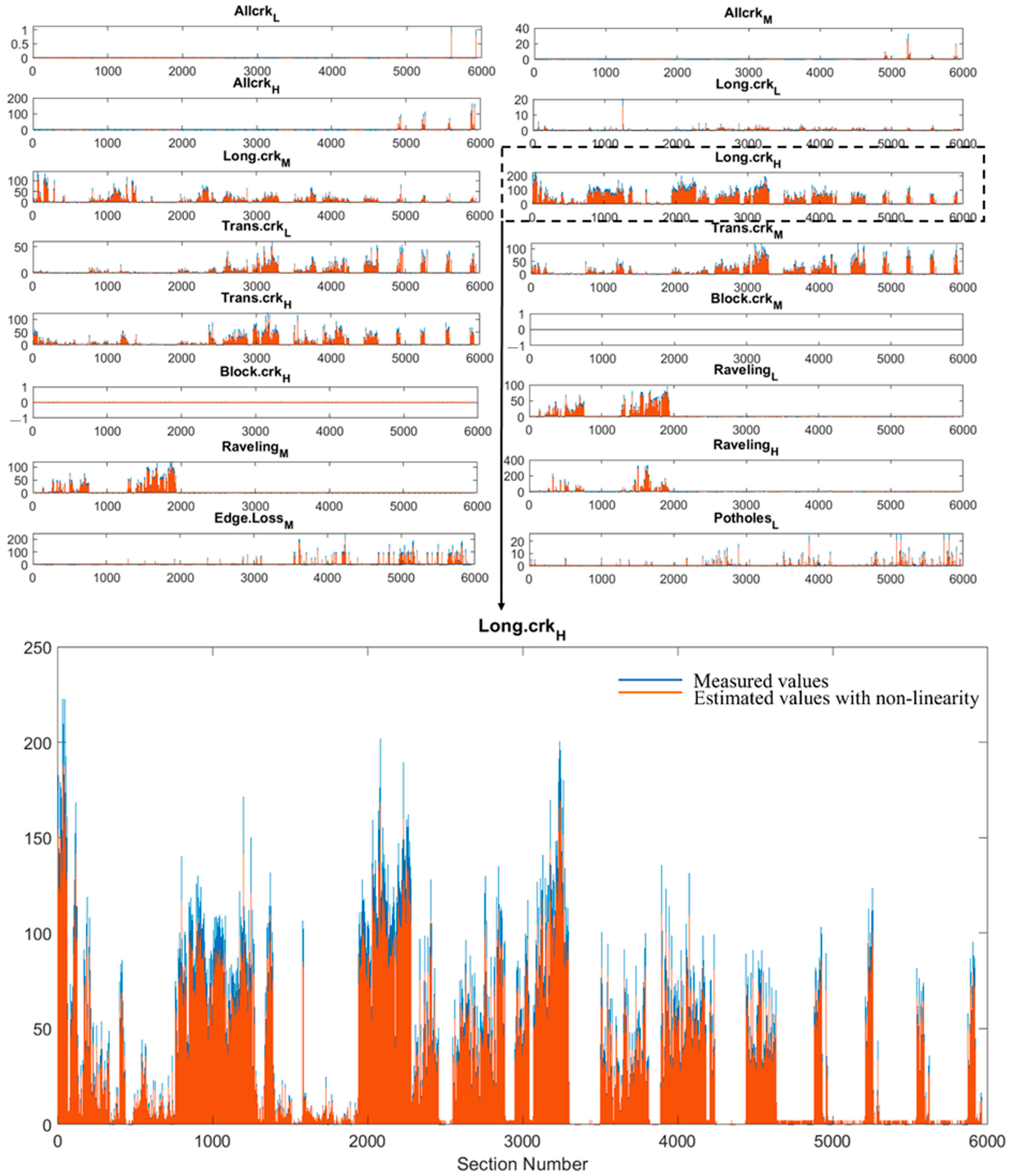
- The related Bayesian estimator is effective in recovering acquisition errors, achieving an overall reduction of the error mean square value of about 25%, with respect to the considered competitors;
- The proposed methodology can be employed to identify sections where the measurements acquired by the 3D laser technology are unreliable related either to the limitations of the automated data collection or data processing software, as extensively discussed in the Introduction section. Indeed, a failure in the measurement system could be revealed when a large difference is computed at the same section between the observed value and the restored one obtained by the Bayesian estimator, i.e., the likelihood of the measured value is small;
- The proposed signal on graph approach selectively improves the quality of the LCMS measurements, as the Bayesian approach achieves a better accuracy in the PCI estimation compared to the LCMS PCI.
Author Contributions
Funding
Institutional Review Board Statement
Informed Consent Statement
Data Availability Statement
Conflicts of Interest
References
- Cafiso, S.; Di Graziano, A.; Goulias, D.G.; D’Agostino, C. Distress and Profile Data Analysis for Condition Assessment in Pavement Management Systems. Int. J. Pavement Res. Technol. 2019, 12, 527–536. [Google Scholar] [CrossRef]
- Queiroz, C.A.; Gautam, S. Road Infrastructure and Economic Development: Some Diagnostic Indicators; World Bank Publications: Washington, DC, USA, 1992; Volume 921. [Google Scholar]
- Ragnoli, A.; De Blasiis, M.; Di Benedetto, A. Pavement Distress Detection Methods: A Review. Infrastructures 2018, 3, 58. [Google Scholar] [CrossRef] [Green Version]
- Bruno, S.; Vita, L.; Loprencipe, G. Development of a GIS-Based Methodology for the Management of Stone Pavements Using Low-Cost Sensors. Sensors 2022, 22, 6560. [Google Scholar] [CrossRef] [PubMed]
- Hafizyar, R.; Mosaberpanah, M. Evaluation of Flexible Road Pavement Condition Index and Life Cycle Cost Analysis of Pavement Maintenance: A Case Study in Kabul Afghanistan. Int. J. Sci. Eng. Res. 2018, 9, 1909. [Google Scholar]
- D6433–20; Standard Practice for Roads and Parking Lots Pavement Condition Index Surveys. ASTM International: West Conshohocken, PA, USA, 2020.
- D5340–20; Standard Test Method for Airport Pavement Condition Index Surveys. ASTM International: West Conshohocken, PA, USA, 2020.
- Fan, Z.; Lin, H.; Li, C.; Su, J.; Bruno, S.; Loprencipe, G. Use of Parallel ResNet for High-Performance Pavement Crack Detection and Measurement. Sustainability 2022, 14, 1825. [Google Scholar] [CrossRef]
- Cafiso, S.; D’Agostino, C.; Delfino, E.; Montella, A. From Manual to Automatic Pavement Distress Detection and Classification. In Proceedings of the 2017 5th IEEE International Conference on Models and Technologies for Intelligent Transportation Systems (MT-ITS), Naples, Italy, 26–28 June 2017; IEEE: Piscataway, NJ, USA, 2017; pp. 433–438. [Google Scholar]
- Loprencipe, G.; de Almeida Filho, F.G.V.; de Oliveira, R.H.; Bruno, S. Validation of a Low-Cost Pavement Monitoring Inertial-Based System for Urban Road Networks. Sensors 2021, 21, 3127. [Google Scholar] [CrossRef]
- Zakeri, H.; Nejad, F.M.; Fahimifar, A. Image Based Techniques for Crack Detection, Classification and Quantification in Asphalt Pavement: A Review. Arch. Comput. Methods Eng. 2017, 24, 935–977. [Google Scholar] [CrossRef]
- Miśkiewicz, M.; Daszkiewicz, K.; Lachowicz, J.; Tysiac, P.; Jaskula, P.; Wilde, K. Nondestructive Methods Complemented by FEM Calculations in Diagnostics of Cracks in Bridge Approach Pavement. Autom. Constr. 2021, 128, 103753. [Google Scholar] [CrossRef]
- Du, Z.; Yuan, J.; Xiao, F.; Hettiarachchi, C. Application of Image Technology on Pavement Distress Detection: A Review. Measurement 2021, 184, 109900. [Google Scholar] [CrossRef]
- Mataei, B.; Nejad, F.M.; Zakeri, H. Automatic Pavement Texture Measurement Using a New 3D Image-Based Profiling System. Measurement 2022, 199, 111456. [Google Scholar] [CrossRef]
- Saad, A.M.; Tahar, K.N. Identification of Rut and Pothole by Using Multirotor Unmanned Aerial Vehicle (UAV). Measurement 2019, 137, 647–654. [Google Scholar] [CrossRef]
- Garilli, E.; Bruno, N.; Autelitano, F.; Roncella, R.; Giuliani, F. Automatic Detection of Stone Pavement’s Pattern Based on UAV Photogrammetry. Autom. Constr. 2021, 122, 103477. [Google Scholar] [CrossRef]
- Hoang, N.-D. Automatic Detection of Asphalt Pavement Raveling Using Image Texture Based Feature Extraction and Stochastic Gradient Descent Logistic Regression. Autom. Constr. 2019, 105, 102843. [Google Scholar] [CrossRef]
- Abbondati, F.; Biancardo, S.A.; Veropalumbo, R.; Dell’Acqua, G. Surface Monitoring of Road Pavements Using Mobile Crowdsensing Technology. Measurement 2021, 171, 108763. [Google Scholar] [CrossRef]
- Kheirati, A.; Golroo, A. Low-Cost Infrared-Based Pavement Roughness Data Acquisition for Low Volume Roads. Autom. Constr. 2020, 119, 103363. [Google Scholar] [CrossRef]
- Sattar, S.; Li, S.; Chapman, M. Developing a near Real-Time Road Surface Anomaly Detection Approach for Road Surface Monitoring. Measurement 2021, 185, 109990. [Google Scholar] [CrossRef]
- Ouma, Y.O.; Hahn, M. Pothole Detection on Asphalt Pavements from 2D-Colour Pothole Images Using Fuzzy c -Means Clustering and Morphological Reconstruction. Autom. Constr. 2017, 83, 196–211. [Google Scholar] [CrossRef]
- Zhang, D.; Zou, Q.; Lin, H.; Xu, X.; He, L.; Gui, R.; Li, Q. Automatic Pavement Defect Detection Using 3D Laser Profiling Technology. Autom. Constr. 2018, 96, 350–365. [Google Scholar] [CrossRef]
- Dan, D.; Dan, Q. Automatic Recognition of Surface Cracks in Bridges Based on 2D-APES and Mobile Machine Vision. Measurement 2021, 168, 108429. [Google Scholar] [CrossRef]
- Li, G.; Liu, Q.; Ren, W.; Qiao, W.; Ma, B.; Wan, J. Automatic Recognition and Analysis System of Asphalt Pavement Cracks Using Interleaved Low-Rank Group Convolution Hybrid Deep Network and SegNet Fusing Dense Condition Random Field. Measurement 2021, 170, 108693. [Google Scholar] [CrossRef]
- McNeil, S.; Humplick, F. Evaluation of Errors in Automated Pavement-Distress Data Acquisition. J. Transp. Eng. 1991, 117, 224–241. [Google Scholar] [CrossRef]
- Dong, Q.; Chen, X.; Dong, S.; Ni, F. Data Analysis in Pavement Engineering: An Overview. IEEE Trans. Intell. Transp. Syst. 2022, 23, 22020–22039. [Google Scholar] [CrossRef]
- Silyanov, V.V.; Sodikov, J.I.; Kiran, R.; Sadikov, A.I. An Overview Road Data Collection, Visualization, and Analysis from the Perspective of Developing Countries. IOP Conf. Ser. Mater. Sci. Eng. 2020, 832, 012056. [Google Scholar] [CrossRef]
- Available online: https://www.pavemetrics.com/applications/road-inspection/lcms2-en/ (accessed on 30 September 2022).
- Pantuso, A.; Loprencipe, G.; Bonin, G.; Teltayev, B.B. Analysis of Pavement Condition Survey Data for Effective Implementation of a Network Level Pavement Management Program for Kazakhstan. Sustainability 2019, 11, 901. [Google Scholar] [CrossRef] [Green Version]
- Tsai, Y.-C.J.; Li, F. Critical Assessment of Detecting Asphalt Pavement Cracks under Different Lighting and Low Intensity Contrast Conditions Using Emerging 3D Laser Technology. J. Transp. Eng. 2012, 138, 649–656. [Google Scholar] [CrossRef]
- Laurent, J.; Hébert, J.F.; Lefebvre, D.; Savard, Y. High-Speed Network Level Road Texture Evaluation Using 1mm Resolution Transverse 3D Profiling Sensors Using a Digital Sand Patch Model. In Proceedings of the 7th International Conference on Maintenance and Rehabilitation of Pavements and Technological Control, Auckland, New Zealand, 28–30 August 2012; pp. 28–30. [Google Scholar]
- Laurent, J.; Hébert, J.F.; Lefebvre, D.; Savard, Y. 3D Laser Road Profiling for the Automated Measurement of Road Surface Conditions and Geometry. In Proceedings of the 7th RILEM International Conference on Cracking in Pavements, Dordrecht, The Netherlands, 20–22 June 2012; Springer: Dordrecht, The Netherlands, 2012. [Google Scholar]
- Sahhaf, S.A.; Rahimi, S. Investigation of Laser Systems Used in Pavement Management Systems (PMS). In Proceedings of the 8th National Congress on Civil Engineering, BabolNoshirvani University of Technology, Babol, Iran, 7–8 May 2014. [Google Scholar]
- Laurent, J.; Lefebvre, D.; Samson, E. Development of a New 3D Transverse Laser Profiling System for the Automatic Measurement of Road Cracks. In Proceedings of the 6th Symposium on Pavement Surface Characteristics, Potoroz, Slovenia, 1 January 2008. [Google Scholar]
- Li, Q.; Zhang, D.; Zou, Q.; Lin, H. 3D Laser Imaging and Sparse Points Grouping for Pavement Crack Detection. In Proceedings of the 2017 25th European Signal Processing Conference (EUSIPCO), Kos Island, Greece, 28 August–2 September 2017; pp. 2036–2040. [Google Scholar]
- Laefer, D.F.; Truong-Hong, L.; Carr, H.; Singh, M. Crack Detection Limits in Unit Based Masonry with Terrestrial Laser Scanning. NDT E Int. 2014, 62, 66–76. [Google Scholar] [CrossRef] [Green Version]
- Wix, R.; Leschinski, R. 3D Technology for Managing Pavements. In Proceedings of the International Public Works Conference, Brisbane, QLD, Australia, 27–29 March 2013. [Google Scholar]
- Laurent, J.; Hébert, J.F.; Talbot, M. Automated Detection of Sealed Cracks Using 2D and 3D Road Surface Data; Pavemetrics Systems Inc.: Québec City, QC, Canada, 2010. [Google Scholar]
- Mulry, B.; Jordan, M.; O’Brien, D.A. Automated Pavement Condition Assessment Using Laser Crack Measurement System (LCMS) on Airfield Pavements in Ireland. In Proceedings of the 9th International Conference on Managing Pavement Assets, Washington, DC, USA, 18–21 May 2015. [Google Scholar]
- Williams, B.; Andre, N.; Bowey, K.; Huynh, K. Integrating Laser Crack Measuring System into the Saskatchewan Pavement Management System. In Proceedings of the TAC 2017: Investing in Transportation: Building Canada’s Economy—2017 Conference and Exhibition of the Transportation Association of Canada, Labrador, NL, Canada, 24–27 September 2017. [Google Scholar]
- Kroizer, A.; Routtenberg, T.; Eldar, Y.C. Bayesian Estimation of Graph Signals. IEEE Trans. Signal Process. 2022, 70, 2207–2223. [Google Scholar] [CrossRef]
- Colonnese, S.; Lorenzo, P.D.; Cattai, T.; Scarano, G.; Fallani, F.D.V. A Joint Markov Model for Communities, Connectivity and Signals Defined Over Graphs. IEEE Signal Process. Lett. 2020, 27, 1160–1164. [Google Scholar] [CrossRef]
- Pantuso, A.; Flintsch, G.W.; Katicha, S.W.; Loprencipe, G. Development of Network-Level Pavement Deterioration Curves Using the Linear Empirical Bayes Approach. Int. J. Pavement Eng. 2021, 22, 780–793. [Google Scholar] [CrossRef] [Green Version]
- Doğan, G.; Ergen, B. A New Mobile Convolutional Neural Network-Based Approach for Pixel-Wise Road Surface Crack Detection. Measurement 2022, 195, 111119. [Google Scholar] [CrossRef]
- Bonin, G.; Folino, N.; Loprencipe, G.; Oliverio Rossi, G.; Polizzotti, S.; Teltayev, B. Development of a Road Asset Management System in Kazakhstan. In Proceedings of the TIS 2017 International Congress on Transport Infrastructure and Systems, Rome, Italy, 10–12 April 2017; pp. 10–12. [Google Scholar]
- Di Mascio, P.; Moretti, L. Implementation of a Pavement Management System for Maintenance and Rehabilitation of Airport Surfaces. Case Stud. Constr. Mater. 2019, 11, e00251. [Google Scholar] [CrossRef]
- Canestrari, F.; Ingrassia, L.P. A Review of Top-down Cracking in Asphalt Pavements: Causes, Models, Experimental Tools and Future Challenges. J. Traffic Transp. Eng. 2020, 7, 541–572. [Google Scholar] [CrossRef]
- Cation, K.A.; Shahin, M.Y.; Scullion, T.; Lytton, R.L. Development of a Preventive Maintenance Algorithm for Use in Pavement Management Systems; Transportation Research Board: Washington, DC, USA, 1987; pp. 1–11. ISBN 0-309-04503-7. [Google Scholar]
- van de Schoot, R.; Depaoli, S.; King, R.; Kramer, B.; Märtens, K.; Tadesse, M.G.; Vannucci, M.; Gelman, A.; Veen, D.; Willemsen, J. Bayesian Statistics and Modelling. Nat. Rev. Methods Primers 2021, 1, 1–26. [Google Scholar] [CrossRef]
- Cao, W.; Liu, Q.; He, Z. Review of Pavement Defect Detection Methods. IEEE Access 2020, 8, 14531–14544. [Google Scholar] [CrossRef]
- Cano-Ortiz, S.; Pascual-Muñoz, P.; Castro-Fresno, D. Machine Learning Algorithms for Monitoring Pavement Performance. Autom. Constr. 2022, 139, 104309. [Google Scholar] [CrossRef]
- Yao, L.; Leng, Z.; Jiang, J.; Ni, F. Modelling of pavement performance evolution considering uncertainty and interpretability: A machine learning based framework. Int. J. Pavement Eng. 2021, 1–16. [Google Scholar] [CrossRef]
- Jacovitti, G.; Panci, G.; Scarano, G. Bussgang-Zero Crossing Equalization: An Integrated HOS-SOS Approach. IEEE Trans. Signal Process. 2001, 49, 2798–2812. [Google Scholar] [CrossRef]
- Panci, G.; Campisi, P.; Colonnese, S.; Scarano, G. Multichannel Blind Image Deconvolution Using the Bussgang Algorithm: Spatial and Multiresolution Approaches. IEEE Trans. Image Process. 2003, 12, 1324–1337. [Google Scholar] [CrossRef]
- LeCam, L. On the Distribution of Sums of Independent Random Variables. In Bernoulli 1713, Bayes 1763, Laplace 1813; Springer: Berlin/Heidelberg, Germany, 1965; pp. 179–202. [Google Scholar]
- Poor, H.V. An Introduction to Signal Detection and Estimation; Springer Science & Business Media: Boston, NY, USA, 2013; ISBN 1-4757-2341-5. [Google Scholar]
- Hobza, T.; Pardo, L.; Vajda, I. Robust Median Estimator in Logistic Regression. J. Stat. Plan. Inference 2008, 138, 3822–3840. [Google Scholar] [CrossRef]
- Loprencipe, G.; Pantuso, A. A Specified Procedure for Distress Identification and Assessment for Urban Road Surfaces Based on PCI. Coatings 2017, 7, 65. [Google Scholar] [CrossRef]


| ID | ASTM Name | Degree of Severity | Unit of Measure | Cause |
|---|---|---|---|---|
| 1 | Alligator cracking | Low | m2 | Load |
| 2 | Medium | m2 | Load | |
| 3 | High | m2 | Load | |
| 4 | Rutting | Low | m2 | Load |
| 5 | Medium | m2 | Load | |
| 6 | High | m2 | Load | |
| 7 | Longitudinal cracking | Low | m | Climatic/Construction defect |
| 8 | Medium | m | Climatic/Construction defect | |
| 9 | High | m | Climatic/Construction defect | |
| 10 | Transverse cracking | Low | m | Climatic/Construction defect |
| 11 | Medium | m | Climatic/Construction defect | |
| 12 | High | m | Climatic/Construction defect | |
| 13 | Block cracking | Medium | m2 | Climatic |
| 14 | High | m2 | Climatic | |
| 15 | Raveling | Low | m2 | Bituminous mixture low quality |
| 16 | Medium | m2 | Bituminous mixture low quality | |
| 17 | High | m2 | Bituminous mixture low quality | |
| 18 | Lane/Shoulder Drop-off | Medium | m | Climatic/Poor construction |
| 19 | Potholes | Low | [-] | Traffic, load |
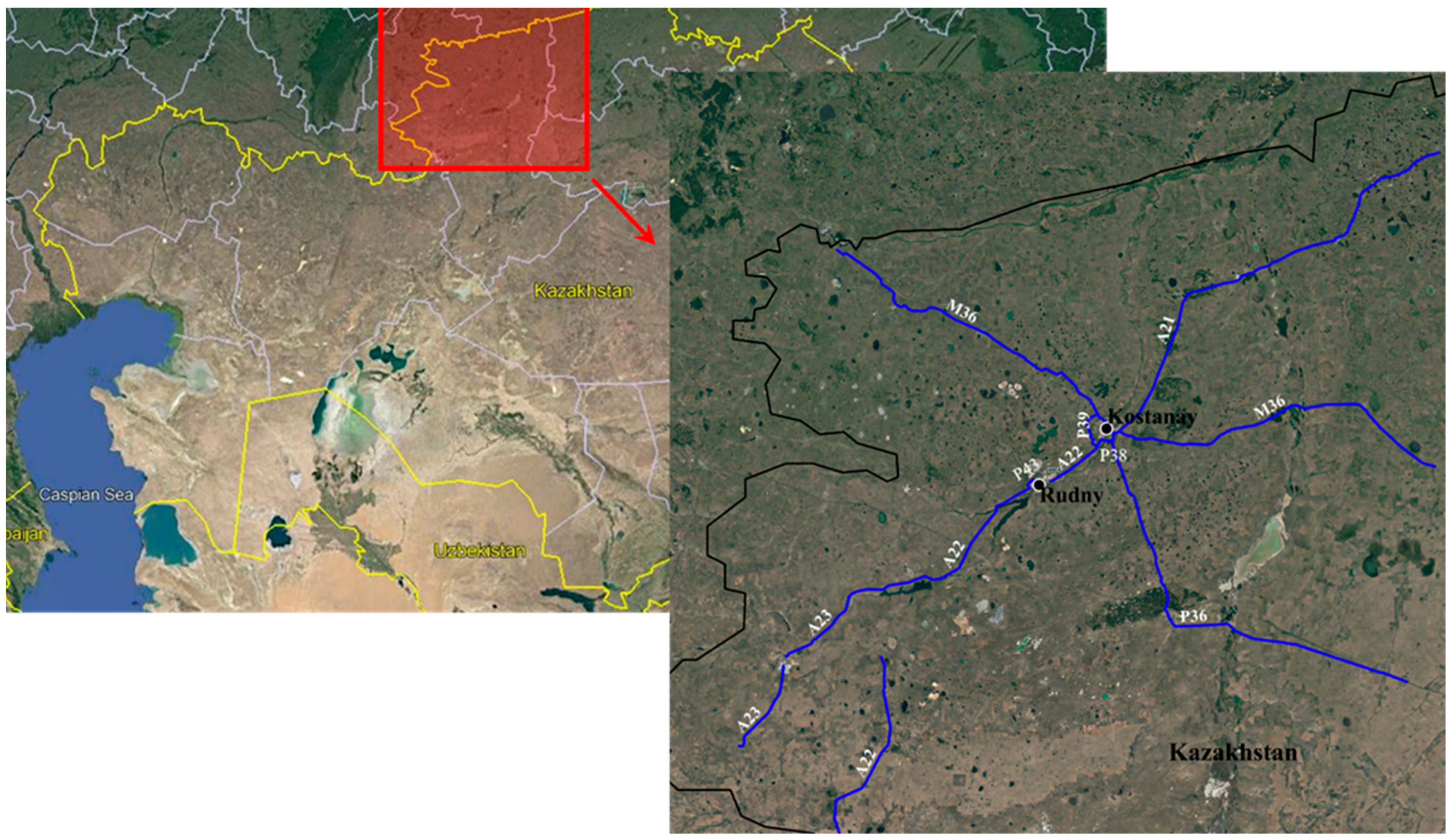
| Road Name | Category | Direction |
|---|---|---|
| M36 | International Highway | Border of Russia—Kostanay—Astana—Karaganda—Almaty |
| A21 | National Highway | Mamlyutka—Kostanay |
| A22 | National Highway | Karabutak—Komsomol’skoe, Kazakhstan—Denisovka—Rudny, Kazakhstan—Kostanay |
| A23 | National Highway | Denisovka—Zhetikara—Muktikol |
| P36 | Regional Highway | Kostanay—Auliekol—Surgan |
| P38 | Regional Highway | Kostanay Southern Bypass (At Minchurinskoe) |
| P39 | Regional Highway | Kostanay Western Bypass |
| P43 | Regional Highway | Rudny West Bypass |
Publisher’s Note: MDPI stays neutral with regard to jurisdictional claims in published maps and institutional affiliations. |
© 2022 by the authors. Licensee MDPI, Basel, Switzerland. This article is an open access article distributed under the terms and conditions of the Creative Commons Attribution (CC BY) license (https://creativecommons.org/licenses/by/4.0/).
Share and Cite
Bruno, S.; Colonnese, S.; Scarano, G.; Del Serrone, G.; Loprencipe, G. Pavement Distress Estimation via Signal on Graph Processing. Sensors 2022, 22, 9183. https://doi.org/10.3390/s22239183
Bruno S, Colonnese S, Scarano G, Del Serrone G, Loprencipe G. Pavement Distress Estimation via Signal on Graph Processing. Sensors. 2022; 22(23):9183. https://doi.org/10.3390/s22239183
Chicago/Turabian StyleBruno, Salvatore, Stefania Colonnese, Gaetano Scarano, Giulia Del Serrone, and Giuseppe Loprencipe. 2022. "Pavement Distress Estimation via Signal on Graph Processing" Sensors 22, no. 23: 9183. https://doi.org/10.3390/s22239183