
DRL-OS: A Deep Reinforcement Learning-Based Offloading Scheduler in Mobile Edge Computing

Abstract
:1. Introduction
- (1)
- Task segmentation is assumed to be a complex process because simple task segmentation may not be realistic owing to the dependency between bits in the task. We consider the default queue system in the SD and MEC. Each task can be processed by core, and processed as many as the number of multi core.
- (2)
- Unlike previous studies that focused on delay tolerance, this study considers delay-sensitive tasks with a variable deadline. This is because a task will consume energy or will be delayed once task processing is initiated, even if it does not meet the deadline or cannot be completed due to lack of energy.
- (3)
- Successful processing, latency, and energy of the task should be considered for local and remote processing. If it is difficult to process the task, the SD drops the task without processing it.
- (4)
- The system is highly complex because it has several variables that need to be considered to reflect realistic scenarios. Therefore, we propose the deep-reinforcement-learning-based offloading scheduler (DRL-OS) approach. The DRL is used to obtain the task offloading policy from the information of the task to be processed in an SD, network, and MEC state.
2. Related Work
2.1. Computation Offloading
2.2. Types of Reinforcement Learning
2.2.1. Reinforcement Learning
2.2.2. Q-Learning
2.2.3. Deep Q-Network
2.2.4. Double Deep Q-Network
2.2.5. Dueling Deep Q-Network
3. System Model
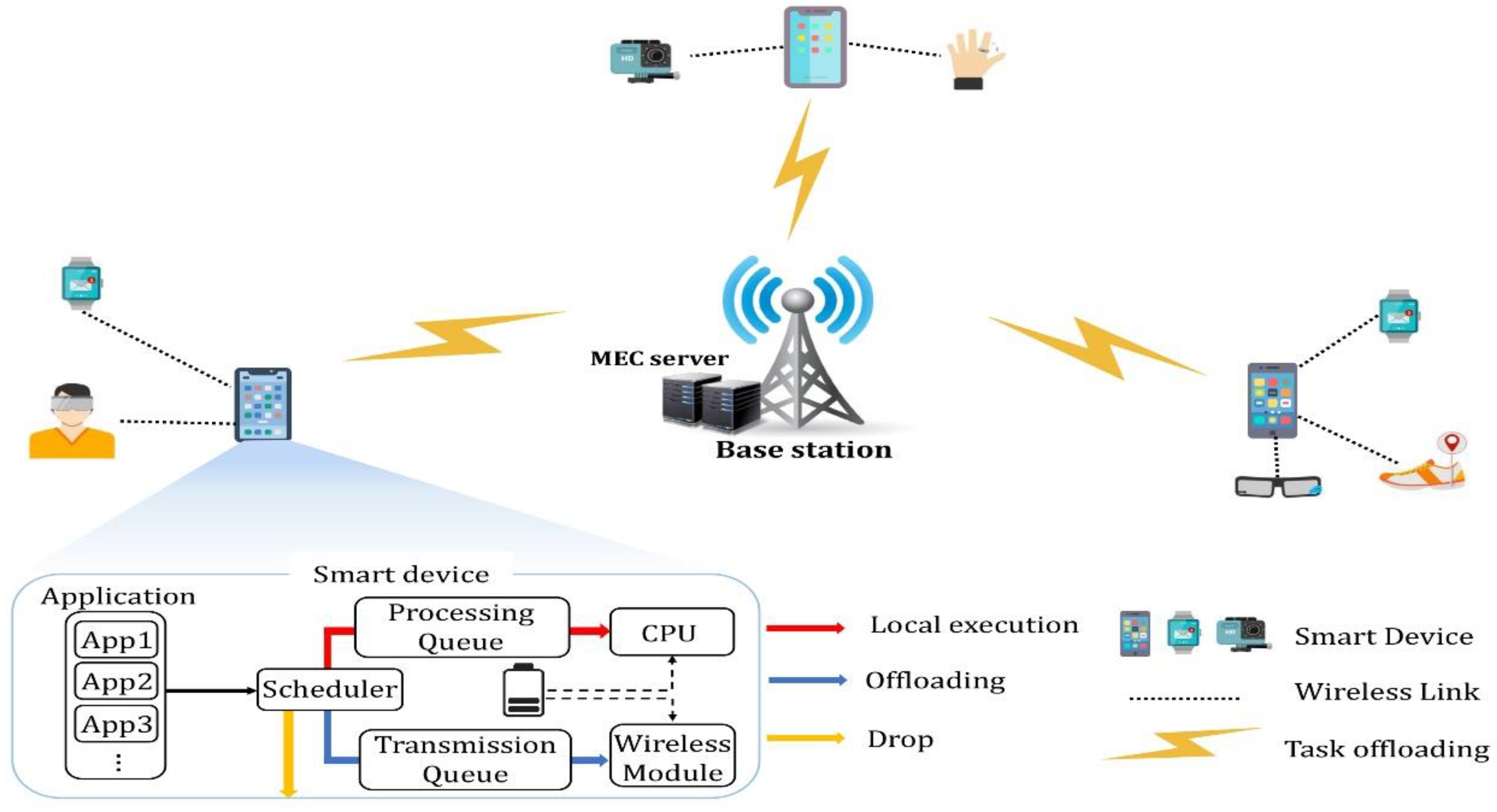
3.1. Components
- It is assumed that the SDs are connected to one MEC server through 5G or Wi-Fi. SDs offload tasks to the wireless network.
- We assumed that the SD is either fixed or has low mobility. Some of them are sensor network devices or are used by users resulting in low mobility.
- Each SD was assumed to have the same processing performance. The number of WDs connected to the SD and the task size are different. Therefore, even if the performance of the device is the same, different results can be obtained due to external influences.
- It was assumed that tasks could be processed and transmitted only in the first created unit of size. In addition, task segmentation is assumed difficult because of the dependency between bits in the task. Therefore, the task is sent with full offloading.
3.2. Computation Model
3.2.1. Local Computing
3.2.2. Remote Edge Computing
4. DRL-Based Offloading Scheduler
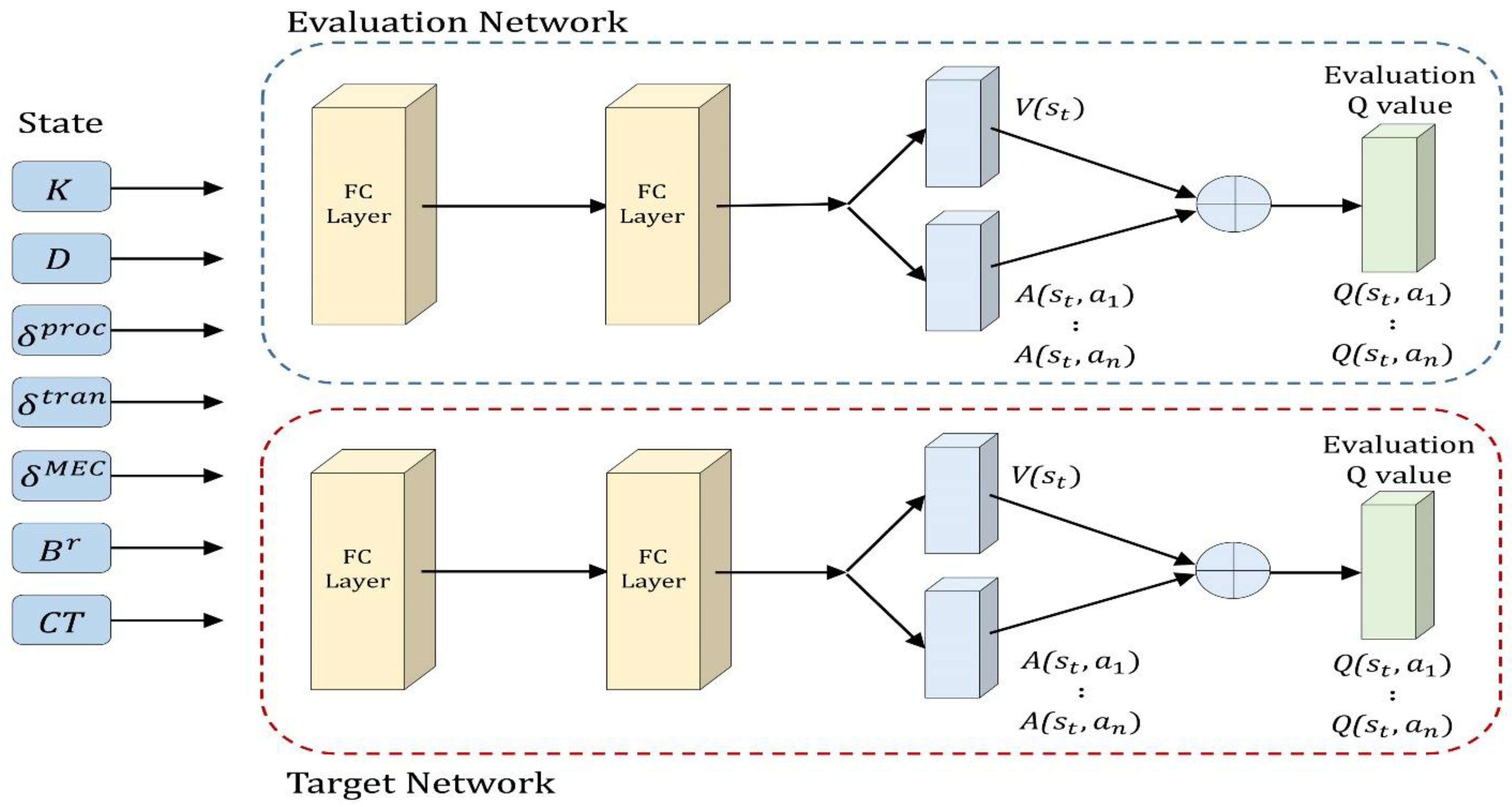
4.1. State Space
4.2. Action Space
4.3. Reward
4.4. Architecture of DRL-Based Offloading Scheduler
4.4.1. D3QN Architecture
4.4.2. Proposed Scheduler
5. Experimental Results
5.1. Experimental Setting
- A local scheme which computes tasks locally by allowing offloading decision parameter without task offloading;
- A remote scheme which processes tasks by offloading them to an MEC server through a transmission queue instead of processing them locally;
- A random scheme [41] which performs computation by randomly selecting local and offloading regardless of the task size and network condition;
- An optimal scheme selects and performs optimal decisions by determining the minimum energy and latency costs;
- A rule-based scheme [14] is an offloading decision method that considers the queue status to minimize the latency.
5.2. Simulation Results and Discussion
5.2.1. Convergence Analysis
5.2.2. Impact of Task Size Analysis
5.2.3. Impact of Deadline Analysis
6. Conclusions
Author Contributions
Funding
Institutional Review Board Statement
Informed Consent Statement
Data Availability Statement
Acknowledgments
Conflicts of Interest
Appendix A

| Work Area | Aim | Related Work | Proposed Solution |
|---|---|---|---|
| Latency based offloading | Minimize the time consumed by the processing of delay-sensitive applications | [13] | The offloading problem to minimize the expected long-term cost (latency and deadline), while considering delay-sensitive tasks in a total offloading situation |
| [15] | A heuristic program segmentation algorithm in an MCC framework to use the method based on the concept of load balancing | ||
| [16] [17] | A latency-aware workload offloading strategy in terms of a new cloudlet network to minimize waiting time Delay-tolerant and delay-sensitive tasks to achieve optimized service delay and revenue | ||
| Energy based offloading | Reduce the energy by identifying the cause of energy, considering the battery of a device with portability constraints | [18] [19] [20] [21] [22] | An energy-optimal mobile computing framework to process applications by locally optimized energy or through offloading Data transmission schedules to reduce the total energy consumption of mobile devices in an MCC system An optimal computation offloading algorithm for mobile users in intermittently connected cloudlet systems The variability of features of mobile devices and user preferences to research an efficient energy computational offloading management method The offloading energy optimization problem, which considered the computation capabilities |
| Cost based offloading | Reduce the cost (i.e., improve efficiency) by considering both waiting time and energy | [23] | Minimize the energy consumption of mobile devices through a joint communication and computation resource allocation algorithm in MEC System |
| [24] | An algorithm that minimized the offloading energy consumption according to the task deadline | ||
| [25] | An algorithm that optimized the decision on the allocation of computational re-sources of the offloading and MEC of mobile devices | ||
| [26] | A distributed offloading algorithm to resolve competition for wireless channels among mobile devices |
References
- Li, M.; Si, P.; Zhang, Y. Delay-tolerant data traffic to software-defined vehicular networks with mobile edge computing in smart city. IEEE Trans. Veh. Technol. 2018, 67, 9073–9086. [Google Scholar] [CrossRef]
- Hao, W.; Zeng, M.; Sun, G.; Xiao, P. Edge cache-assisted secure low-latency millimeter-wave transmission. IEEE Internet Things J. 2019, 7, 1815–1825. [Google Scholar] [CrossRef]
- Dian, F.J.; Vahidnia, R.; Rahmati, A. Wearables and the Internet of Things (IoT), applications, opportunities, and challenges: A Survey. IEEE Access. 2020, 8, 69200–69211. [Google Scholar] [CrossRef]
- Mao, Y.; You, C.; Zhang, J.; Huang, K.; Letaief, K.B. A survey on mobile edge computing: The communication perspective. IEEE Commun. Surv. Tutor. 2017, 19, 2322–2358. [Google Scholar] [CrossRef] [Green Version]
- Nguyen, Q.-H.; Dressler, F. A smartphone perspective on computation offloading—A survey. Comput. Commun. 2020, 159, 133–154. [Google Scholar] [CrossRef]
- Zheng, J.; Cai, Y.; Wu, Y.; Shen, X. Dynamic computation offloading for mobile cloud computing: A stochastic game-theoretic approach. IEEE Trans. Mob. Comput. 2018, 18, 771–786. [Google Scholar] [CrossRef]
- Hamdan, S.; Ayyash, M.; Almajali, S. Edge-computing architectures for internet of things applications: A survey. Sensors 2020, 20, 6441. [Google Scholar] [CrossRef]
- Porambage, P.; Okwuibe, J.; Liyanage, M.; Ylianttila, M.; Taleb, T. Survey on multi-access edge computing for internet of things realization. IEEE Commun. Surv. Tutor. 2018, 20, 2961–2991. [Google Scholar] [CrossRef] [Green Version]
- Kuru, K. Planning the future of smart cities with swarms of fully autonomous unmanned aerial vehicles using a novel framework. IEEE Access. 2021, 9, 6571–6595. [Google Scholar] [CrossRef]
- Eom, H.; Juste, P.S.; Figueiredo, R.; Tickoo, O.; Illikkal, R.; Iyer, R. Machine learning-based runtime scheduler for mobile offloading framework. In Proceedings of the 6th International Conference on Utility and Cloud Computing, Washington, DC, USA, 9–12 December 2013; Volume 2013, pp. 17–25. [Google Scholar] [CrossRef]
- Wang, C.; Liang, C.; Yu, F.R.; Chen, Q.; Tang, L. Computation offloading and resource allocation in wireless cellular networks with mobile edge computing. IEEE Trans. Wirel. Commun. 2017, 16, 4924–4938. [Google Scholar] [CrossRef]
- Ali, Z.; Jiao, L.; Baker, T.; Abbas, G.; Abbas, Z.H.; Khaf, S. A deep learning approach for energy efficient computational offloading in mobile edge computing. IEEE Access. 2019, 7, 149623–149633. [Google Scholar] [CrossRef]
- Tang, M.; Wong, V.W.S. Deep reinforcement learning for task offloading in mobile edge computing systems. IEEE Trans. Mob. Comput. 2020, 21, 1985–1997. [Google Scholar] [CrossRef]
- Liu, J.; Mao, Y.; Zhang, J.; Letaief, K.B. Delay-optimal computation task scheduling for mobile-edge computing systems. In Proceedings of the IEEE International Symposium on Information Theory (ISIT), Barcelona, Spain, 10–15 July 2016; Volume 2016, pp. 1451–1455. [Google Scholar] [CrossRef] [Green Version]
- Jia, M.; Cao, J.; Yang, L. Heuristic offloading of concurrent tasks for computation-intensive applications in mobile cloud computing. In Proceedings of the IEEE Conference on Computer Communications Workshops (INFOCOM WKSHPS), Toronto, Canada, 27 April–2 May 2014; Volume 2014, pp. 352–357. [Google Scholar] [CrossRef]
- Sun, X.; Ansari, N. Latency aware workload offloading in the cloudlet network. IEEE Commun. Lett. 2017, 21, 1481–1484. [Google Scholar] [CrossRef]
- Samanta, A.; Chang, Z. Adaptive service offloading for revenue maximization in mobile edge computing with delay-constraint. IEEE Internet Things J. 2019, 6, 3864–3872. [Google Scholar] [CrossRef] [Green Version]
- Xiang, X.; Lin, C.; Chen, X. Energy-efficient link selection and transmission scheduling in mobile cloud computing. IEEE Wirel. Commun. Lett. 2014, 3, 153–156. [Google Scholar] [CrossRef]
- Zhang, W.; Wen, Y.; Guan, K.; Kilper, D.; Luo, H.; Wu, D.O. Energy-optimal mobile cloud computing under stochastic wireless channel. IEEE Trans. Wirel. Commun. 2013, 12, 4569–4581. [Google Scholar] [CrossRef]
- Zhang, Y.; Niyato, D.; Wang, P. Offloading in mobile cloudlet systems with intermittent connectivity. IEEE Trans. Mob. Comput. 2015, 14, 2516–2529. [Google Scholar] [CrossRef]
- Guo, F.; Zhang, H.; Ji, H.; Li, X.; Leung, V.C.M. An efficient computation offloading management scheme in the densely deployed small cell networks with mobile edge computing. IEEE ACM Trans. Netw. 2018, 26, 2651–2664. [Google Scholar] [CrossRef]
- Yang, L.; Zhang, H.; Li, M.; Guo, J.; Ji, H. Mobile edge computing empowered energy efficient task offloading in 5G. IEEE Trans. Veh. Technol. 2018, 67, 6398–6409. [Google Scholar] [CrossRef]
- Sardellitti, S.; Scutari, G.; Barbarossa, S. Joint optimization of radio and computational resources for multicell mobile-edge computing. IEEE Trans. Signal Inf. Process. Netw. 2015, 1, 89–103. [Google Scholar] [CrossRef] [Green Version]
- Lyu, X.; Tian, H.; Ni, W.; Zhang, Y.; Zhang, P.; Liu, R.P. Energy-efficient admission of delay-sensitive tasks for mobile edge computing. IEEE Trans. Commun. 2018, 66, 2603–2616. [Google Scholar] [CrossRef] [Green Version]
- Eshraghi, N.; Liang, B. Joint offloading decision and resource allocation with uncertain task computing requirement. In Proceedings of the IEEE Conference on Computer Communications, Paris, France, 29 April–2 May 2019; Volume 2019, pp. 1414–1422. [Google Scholar]
- Yang, L.; Zhang, H.; Li, X.; Ji, H.; Leung, V.C.M. A distributed computation offloading strategy in small-cell networks integrated with mobile edge computing. IEEE ACM Trans. Netw. 2018, 26, 2762–2773. [Google Scholar] [CrossRef]
- Alpaydin, E. Introduction to Machine Learning; MIT Press: Cambridge, MA, USA, 2020. [Google Scholar]
- Lowe, R.; Wu, Y.I.; Tamar, A.; Harb, J.; Pieter Abbeel, O.; Mordatch, I. Multi-agent actor-critic for mixed cooperative-competitive environments. Adv. Neural. Inf. Process. Syst. 2017, 30, 6382–6393. [Google Scholar]
- Watkins, C.J.C.H.; Dayan, P. Q-learning. Mach. Learn. 1992, 8, 279–292. [Google Scholar] [CrossRef]
- Hausknecht, M.; Stone, P. Deep reinforcement learning in parameterized action space. arXiv 2015, arXiv:1511.04143. [Google Scholar]
- Baird, L. Residual algorithms: Reinforcement learning with function approximation. In Machine Learning Proceedings; Morgan Kaufmann: Burlington, MA, USA, 1995; Volume 1995, pp. 30–37. [Google Scholar]
- Van Hasselt, H.; Guez, A.; Silver, D. Deep reinforcement learning with double q-learning. arXiv 2016, arXiv:1509.06461. [Google Scholar] [CrossRef]
- Wang, Z.; Schaul, T.; Hessel, M.; Hasselt, H.; Lanctot, M.; Freitas, N. Dueling network architectures for deep reinforcement learning. In Proceedings of the International Conference on Machine Learning, New York, NY, USA, 19–24 June 2016; pp. 1995–2003. [Google Scholar]
- Oo, T.Z.; Tran, N.H.; Saad, W.; Niyato, D.; Han, Z.; Hong, C.S. Offloading in HetNet: A coordination of interference mitigation, user association, and resource allocation. IEEE Trans. Mob. Comput. 2016, 16, 2276–2291. [Google Scholar] [CrossRef]
- Dos Anjos, J.C.S.; Gross, J.L.G.; Matteussi, K.J.; González, G.V.; Leithardt, V.R.Q.; Geyer, C.F.R. An algorithm to minimize energy consumption and elapsed time for IoT workloads in a hybrid architecture. Sensors 2021, 21, 2914. [Google Scholar] [CrossRef]
- Ren, J.; Yu, G.; He, Y.; Li, G.Y. Collaborative cloud and edge computing for latency minimization. IEEE Trans. Veh. Technol. 2019, 68, 5031–5044. [Google Scholar] [CrossRef]
- Guo, S.; Liu, J.; Yang, Y.; Xiao, B.; Li, Z. Energy-efficient dynamic computation offloading and cooperative task scheduling in mobile cloud computing. IEEE Trans. Mob. Comput. 2018, 18, 319–333. [Google Scholar] [CrossRef]
- Nath, S.; Wu, J.; Yang, J. Delay and energy efficiency tradeoff for information pushing system. IEEE Trans. Green Commun. Netw. 2018, 2, 1027–1040. [Google Scholar] [CrossRef]
- Hessel, M.; Modayil, J.; Van Hasselt, H.; Schaul, T.; Ostrovski, G.; Dabney, W.; Horgan, D.; Piot, B.; Azar, M.; Silver, D. Rainbow: Combining improvements in deep reinforcement learning. In Proceedings of the AAAI Thirty-second AAAI conference on artificial intelligence, New Orleans, LA, USA, 2–7 February 2018; Volume 32. [Google Scholar] [CrossRef]
- Sheng, S.; Chen, P.; Chen, Z.; Wu, L.; Yao, Y. Deep reinforcement learning-based task scheduling in iot edge computing. Sensors 2021, 21, 1666. [Google Scholar] [CrossRef]
- Venieris, S.I.; Panopoulos, I.; Venieris, I.S. OODIn: An optimised on-device inference framework for heterogeneous mobile devices. In Proceedings of the IEEE International Conference on Smart Computing (SMARTCOMP), Irvine, CA, USA, 23–27 August 2021; Volume 2021, pp. 1–8. [Google Scholar] [CrossRef]


| Notation | Description |
|---|---|
| M | A set of SDs |
| Number of CPU cores in the device | |
| K | Size of the task |
| D | Deadline of the task |
| Number of CPU cycles required to process the task | |
| Processing queue of devices | |
| Transmission queue of devices | |
| Processing time of the task by local computing model | |
| Computational capability of SD | |
| Computing power of device | |
| Energy consumption of the task by a local computing model | |
| Time for transmission from the SD to the MEC server | |
| Transmission rate of the SD | |
| Processing time of task by the MEC server | |
| Processing queue of MEC | |
| Computational capability of MEC | |
| Total processing time when task is processed by offloading it to the MEC server in the SD | |
| Energy consumption of task by computational offloading | |
| Transmission power of the SD | |
| Cost of local computing | |
| Cost of processing by offloading | |
| Weighting coefficients |
| Parameters | Settings |
|---|---|
| 5G data rate | 100 Mbps |
| Wi-Fi data rate | 200 Mbps |
| Transmission Power, | 24 dBM [36] |
| Input task size, | 50–450 KB Default: 400 KB |
| Required CPU cycles per bit | 1000 CPU cycles/bit |
| Local computational capability, | CPU cycles/s |
| MEC computational capability, | CPU cycles/s |
| Local CPU core | 8 |
| Edge node CPU core | 128 |
| Weight factor | 0.5 |
| Parameters | Value |
|---|---|
| Learning rate | 0.0005 |
| Discount factor | 0.99 |
| Min epsilon | 0.05 |
| Init epsilon | 0.99 |
| Epsilon decay | 0.00002 |
| Batch size | 64 |
| Episodes | 1200 |
Publisher’s Note: MDPI stays neutral with regard to jurisdictional claims in published maps and institutional affiliations. |
© 2022 by the authors. Licensee MDPI, Basel, Switzerland. This article is an open access article distributed under the terms and conditions of the Creative Commons Attribution (CC BY) license (https://creativecommons.org/licenses/by/4.0/).
Share and Cite
Lim, D.; Lee, W.; Kim, W.-T.; Joe, I. DRL-OS: A Deep Reinforcement Learning-Based Offloading Scheduler in Mobile Edge Computing. Sensors 2022, 22, 9212. https://doi.org/10.3390/s22239212
Lim D, Lee W, Kim W-T, Joe I. DRL-OS: A Deep Reinforcement Learning-Based Offloading Scheduler in Mobile Edge Computing. Sensors. 2022; 22(23):9212. https://doi.org/10.3390/s22239212
Chicago/Turabian StyleLim, Ducsun, Wooyeob Lee, Won-Tae Kim, and Inwhee Joe. 2022. "DRL-OS: A Deep Reinforcement Learning-Based Offloading Scheduler in Mobile Edge Computing" Sensors 22, no. 23: 9212. https://doi.org/10.3390/s22239212