
A Denoising and Fourier Transformation-Based Spectrograms in ECG Classification Using Convolutional Neural Network


Abstract
:1. Introduction
2. Related Work
3. Methodology
3.1. Pre-Processing
3.1.1. Denoising
| Algorithm 1: Denoising |
| Step 1: Step 2: Step 3: Step 4: Step 5: |
3.1.2. Frequency Filtration
| Algorithm 2: Frequency filtration |
| Step 1: Step 2: Step 3: Step 4: |
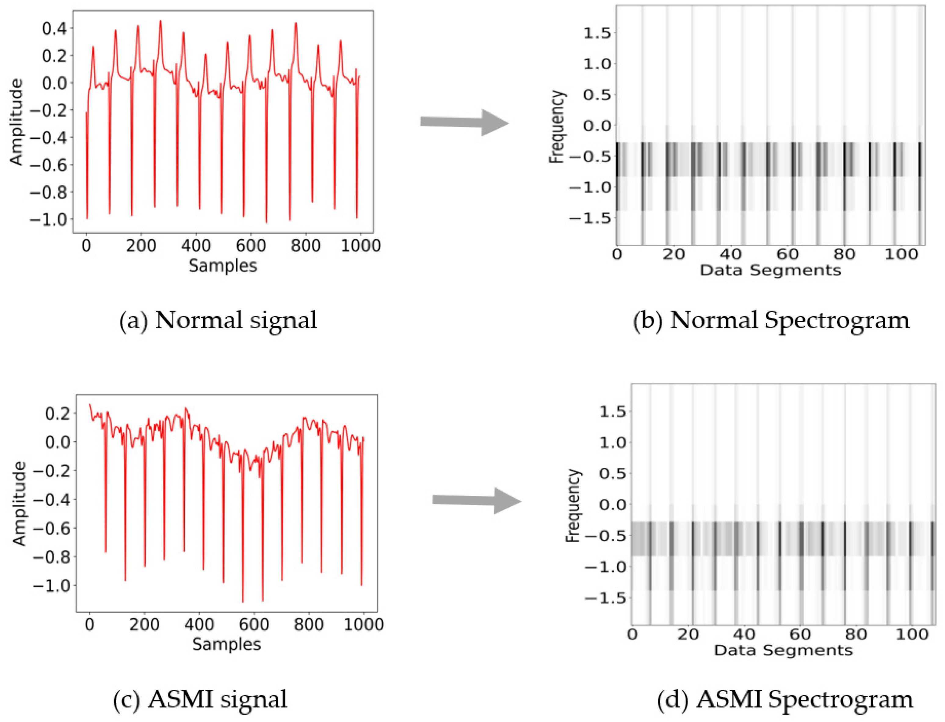
3.1.3. Spectrograms
3.2. Dataset Preparation
3.3. Model Architecture
4. Experimental Setting and Results
4.1. Memory Consumption
4.2. Model Evaluation
4.3. Learning Rate
4.4. Sampling Rate
4.5. Comparison with Existing Methods
5. Conclusions
Author Contributions
Funding
Institutional Review Board Statement
Informed Consent Statement
Data Availability Statement
Conflicts of Interest
References
- Aziz, S.; Ahmed, S.; Alouini, M.-S. ECG-based machine-learning algorithms for heartbeat classification. Sci. Rep. 2021, 11, 18738. [Google Scholar] [CrossRef]
- Raeiatibanadkooki, M.; Quachani, S.; Khalilzade, M.; Bahaadinbeigy, K. Real Time Processing and Transferring ECG Signal by a Mobile Phone. Acta Inform. Med. 2014, 22, 389. [Google Scholar] [CrossRef] [Green Version]
- Serhani, M.A.; TEl Kassabi, H.; Ismail, H.; Nujum Navaz, A. ECG Monitoring Systems: Review, Architecture, Processes, and Key Challenges. Sensors 2020, 20, 1796. [Google Scholar] [CrossRef] [Green Version]
- Søndergaard, M.M.; Riis, J.; Bodker, K.W.; Hansen, S.M.; Nielsen, J.; Graff, C.; Pietersen, A.H.; Nielsen, J.B.; Tayal, B.; Polcwiartek, C.; et al. Associations between left bundle branch block with different PR intervals, QRS durations, heart rates and the risk of heart failure: A register-based cohort study using ECG data from the primary care setting. Open Heart 2021, 8, e001425. [Google Scholar] [CrossRef]
- Liu, Y.; Ping, J.; Qiu, L.; Sun, C.; Chen, M. Comparative analysis of ischemic changes in electrocardiogram and coronary angiography results: A retrospective study. Medicine 2021, 100, e26007. [Google Scholar] [CrossRef]
- Udawat, A.S.; Singh, P. An automated detection of atrial fibrillation from single-lead ECG using HRV features and machine learning. J. Electrocardiol. 2022, 71, 70–81. [Google Scholar] [CrossRef]
- Bacharova, L. ECG in left ventricular hypertrophy: A change in paradigm from assessing left ventricular mass to its electrophysiological properties. J. Electrocardiol. 2022, 73, 153–156. [Google Scholar] [CrossRef]
- Liu, Y.-L.; Lin, C.-S.; Cheng, C.-C.; Lin, C. A Deep Learning Algorithm for Detecting Acute Pericarditis by Electrocardiogram. J. Pers. Med. 2022, 12, 1150. [Google Scholar] [CrossRef]
- Bhattarai, S.; Chhabra, L.; Hashmi, M.F.; Matalgah, M.M. Anteroseptal Myocardial Infarction. In StatPearls; StatPearls Publishing: Treasure Island, FL, USA, 2022. Available online: https://www.ncbi.nlm.nih.gov/books/NBK540996/ (accessed on 20 July 2022).
- Gupta, V.; Mittal, M. A Comparison of ECG Signal Pre-processing Using FrFT, FrWT and IPCA for Improved Analysis. IRBM 2019, 40, 145–156. [Google Scholar] [CrossRef]
- Gupta, V.; Mittal, M.; Mittal, V. Performance Evaluation of Various Pre-Processing Techniques for R-Peak Detection in ECG Signal. IETE J. Res. 2020, 68, 3267–3282. [Google Scholar] [CrossRef]
- Mortezaee, M.; Mortezaie, Z.; Abolghasemi, V. An Improved SSA-Based Technique for EMG Removal from ECG. IRBM 2019, 40, 62–68. [Google Scholar] [CrossRef]
- Al-Ghraibah, A.; El-Sharo, S.; Al-Nabulsi, J.; Matalgah, M.M. Evaluation of the carotid artery using wavelet-based analysis of the pulse wave signal. Int. J. Elec. Comp. Eng. 2022, 12, 1456–1467. [Google Scholar]
- Stokfiszewski, K.; Wieloch, K.; Yatsymirskyy, M. An efficient implementation of one-dimensional discrete wavelet transforms algorithms for GPU architectures. J. Supercomput. 2022, 78, 11539–11563. [Google Scholar] [CrossRef]
- Fars, S.; Thomas, S. An efficient ECG Denoising method using Discrete Wavelet with Savitzky-Golay filter. Curr. Dir. Biomed. Eng. 2019, 5, 385–387. [Google Scholar] [CrossRef]
- Gualsaqui, M.; Vizcaíno, I.; Proaño, V.; Flores, M. ECG signal denoising using discrete wavelet transform: A comparative analysis of threshold values and functions. MASKANA 2018, 9, 105–114. [Google Scholar] [CrossRef]
- Dautov, Ç.P.; Özerdem, M.S. Wavelet transform and signal denoising using Wavelet method. In Proceedings of the 2018 26th Signal Processing and Communications Applications Conference (SIU), Izmir, Turkey, 2–5 May 2018; pp. 1–4. [Google Scholar] [CrossRef]
- Zhang, R.; Liu, X.; Zheng, Y.; Lv, H.; Li, B.; Yang, S.; Tan, Y. Time-frequency synchroextracting transform. IET Signal Process 2022, 16, 117–131. [Google Scholar] [CrossRef]
- Yan, J.; Laflamme, S.; Singh, P.; Sadhu, A.; Dodson, J. A Comparison of Time-Frequency Methods for Real-Time Application to High-Rate Dynamic Systems. Vibration 2020, 3, 204–216. [Google Scholar] [CrossRef]
- Kang, M.; Shin, S.; Jung, J.; Kim, Y.T. Classification of Mental Stress Using CNN-LSTM Algorithms with Electrocardiogram Signals. J. Healthc. Eng. 2021, p. e9951905. Available online: https://www.hindawi.com/journals/jhe/2021/9951905/ (accessed on 10 May 2022).
- Wang, T.; Lu, C.; Sun, Y.; Yang, M.; Liu, C.; Ou, C. Automatic ECG Classification Using Continuous Wavelet Transform and Convolutional Neural Network. Entropy 2021, 23, 119. [Google Scholar] [CrossRef]
- Jeon, H.; Jung, Y.; Lee, S.; Jung, Y. Area-Efficient Short-Time Fourier Transform Processor for Time–Frequency Analysis of Non-Stationary Signals. Appl. Sci. 2020, 10, 7208. [Google Scholar] [CrossRef]
- Mateo, C.; Talavera, J.A. Short-Time Fourier Transform with the Window Size Fixed in the Frequency Domain (STFT-FD): Implementation. SoftwareX 2018, 8, 5–8. [Google Scholar] [CrossRef]
- STFT Signal—SciPy v1.8.1 Manual. Available online: https://docs.scipy.org/doc/scipy/reference/generated/scipy.signal.stft.html (accessed on 20 July 2022).
- Ye, F.; Yang, J. A Deep Neural Network Model for Speaker Identification. Appl. Sci. 2021, 11, 3603. [Google Scholar] [CrossRef]
- Li, W.; Wang, K.; You, L. A Deep Convolutional Network for Multitype Signal Detection and Classification in Spectrogram. Math. Probl. Eng. 2020, 2020, 9797302. [Google Scholar] [CrossRef]
- Li, J.; Si, Y.; Xu, T.; Jiang, S. Deep Convolutional Neural Network Based ECG Classification System Using Information Fusion and One-Hot Encoding Techniques. Math. Probl. Eng. 2018, 2018, 7354081. [Google Scholar] [CrossRef] [Green Version]
- Yadav, S.S.; Jadhav, S.M. Deep convolutional neural network based medical image classification for disease diagnosis. J. Big Data 2019, 6, 13. [Google Scholar] [CrossRef] [Green Version]
- Chiang, C.H.; Weng, C.L.; Chiu, H.W. Automatic classification of medical image modality and anatomical location using convolutional neural network. PLoS ONE 2021, 16, e0253205. [Google Scholar] [CrossRef]
- Reshi, A.A.; Rustam, F.; Mehmood, A.; Alhossan, A.; Alrabiah, Z.; Ahmad, A.; Alsuwailem, H.; Choi, G.S. An Efficient CNN Model for COVID-19 Disease Detection Based on X-Ray Image Classification. Complexity 2021, 2021, 1–12. [Google Scholar] [CrossRef]
- Woźniak, M.; Siłka, J.; Wieczorek, M. Deep neural network correlation learning mechanism for CT brain tumor detection. Neural Comput. Appl. 2021. [Google Scholar] [CrossRef]
- Litjens, G.; Ciompi, F.; Wolterink, J.M.; de Vos, B.D.; Leiner, T.; Teuwen, J.; Išgum, I. State-of-the-Art Deep Learning in Cardiovascular Image Analysis. JACC Cardiovasc. Imaging 2019, 12, 1549–1565. [Google Scholar] [CrossRef]
- Król-Józaga, B. Atrial fibrillation detection using convolutional neural networks on 2-dimensional representation of ECG signal. Biomed. Signal Process. Control. 2022, 74, 103470. [Google Scholar] [CrossRef]
- Huang, J.; Chen, B.; Yao, B.; He, W. ECG Arrhythmia Classification Using STFT-Based Spectrogram and Convolutional Neural Network. IEEE Access 2019, 7, 92871–92880. [Google Scholar] [CrossRef]
- Ullah, A.; Anwar, S.M.; Bilal, M.; Mehmood, R.M. Classification of Arrhythmia by Using Deep Learning with 2-D ECG Spectral Image Representation. Remote Sens. 2020, 12, 1685. [Google Scholar] [CrossRef]
- Liu, G.; Han, X.; Tian, L.; Zhou, W.; Liu, H. ECG quality assessment based on hand-crafted statistics and deep-learned S-transform spectrogram features. Comput. Methods Programs Biomed. 2021, 208, 106269. [Google Scholar] [CrossRef]
- Mishra, A.; Dharahas, G.; Gite, S.; Kotecha, K.; Koundal, D.; Zaguia, A.; Kaur, M.; Lee, H.-N. ECG Data Analysis with Denoising Approach and Customized CNNs. Sensors 2022, 22, 1928. [Google Scholar] [CrossRef]
- AlMahamdy, M.; Riley, H.B. Performance Study of Different Denoising Methods for ECG Signals. Procedia Comput. Sci. 2014, 37, 325–332. [Google Scholar] [CrossRef] [Green Version]
- Gusev, M.; Domazet, E. Optimal DSP bandpass filtering for QRS detection. In Proceedings of the 2018 41st International Convention on Information and Communication Technology, Electronics and Microelectronics (MIPRO), Opatija, Croatia, 12–25 May 2018; pp. 0303–0308. [Google Scholar] [CrossRef]
- Xu, B.; Liu, R.; Shu, M.; Shang, X.; Wang, Y. An ECG Denoising Method Based on the Generative Adversarial Residual Network. Comput. Math. Methods Med. 2021, 1–23. [Google Scholar] [CrossRef]
- Liu, R.; Shu, M.; Chen, C. ECG Signal Denoising and Reconstruction Based on Basis Pursuit. Appl. Sci. 2021, 11, 1591. [Google Scholar] [CrossRef]
- Giełczyk, A.; Marciniak, A.; Tarczewska, M.; Lutowski, Z. Pre-processing methods in chest X-ray image classification. PLoS ONE 2022, 17, e0265949. [Google Scholar] [CrossRef]
- Heidari, M.; Mirniaharikandehei, S.; Khuzani, A.Z.; Danala, G.; Qiu, Y.; Zheng, B. Improving the performance of CNN to predict the likelihood of COVID-19 using chest X-ray images with pre-processing algorithms. Int. J. Med. Inform. 2020, 144, 104284. [Google Scholar] [CrossRef]
- Aboussaleh, I.; Riffi, J.; Mahraz, A.M.; Tairi, H. Brain Tumor Segmentation Based on Deep Learning’s Feature Representation. J. Imaging 2021, 7, 269. [Google Scholar] [CrossRef]
- Nurmaini, S.; Tondas, A.E.; Darmawahyuni, A.; Rachmatullah, M.N.; Effendi, J.; Firdaus, F.; Tutuko, B. signal classification for automated delineation using bidirectional long short-term memory. Inform. Med. Unlocked 2021, 22, 100507. [Google Scholar] [CrossRef]
- Fang, Y.; Shi, J.; Huang, Y.; Zeng, T.; Ye, Y.; Su, L.; Zhu, D.; Huang, J. Electrocardiogram Signal Classification in the Diagnosis of Heart Disease Based on RBF Neural Network. Comput. Math. Methods Med. 2022, 2022, 9251225. [Google Scholar] [CrossRef]
- Fariha, M.A.Z.; Ikeura, R.; Hayakawa, S.; Tsutsumi, S. Analysis of Pan-Tompkins Algorithm Performance with Noisy ECG Signals. J. Phys. Conf. Ser. 2020, 1532, 1. [Google Scholar] [CrossRef]
- Atal, D.K.; Singh, M. Arrhythmia Classification with ECG signals based on the Optimization-Enabled Deep Convolutional Neural Network. Comput. Methods Programs Biomed. 2020, 196, 105607. [Google Scholar] [CrossRef] [PubMed]
- Bat algorithm. Wikipedia. 2020. Available online: https://en.wikipedia.org/wiki/Bat_algorithm (accessed on 5 July 2022).
- PTB-XL, a Large Publicly Available Electrocardiography Dataset v1.0.1. Available online: https://physionet.org/content/ptb-xl/1.0.1/ (accessed on 6 July 2022).
- Singh, B.N.; Tiwari, A.K. Optimal selection of wavelet basis function applied to ECG signal denoising. Digit. Signal Process. 2006, 16, 275–287. [Google Scholar] [CrossRef]
- Discrete Wavelet Transform (DWT)—PyWavelets Documentation. Available online: https://pywavelets.readthedocs.io/en/latest/ref/dwt-discrete-wavelet-transform.html (accessed on 10 May 2022).
- Vantuch, T. Analysis of Time Series Data. Ostrava. Ph.D. Thesis. 2018. VŠB-Technical University of Ostrava, Fakulta Elektrotechniky a Informatiky. Thesis Supervisor Ivan Zelinka. Available online: http://dspace.vsb.cz/bitstream/handle/10084/133114/VAN431_FEI_P1807_1801V001_2018.pdf (accessed on 10 May 2022).
- Jia, H.; Yin, Q.; Lu, M. Blind-noise image denoising with block-matching domain transformation filtering and improved guided filtering. Sci. Rep. 2022, 16195. [Google Scholar] [CrossRef] [PubMed]


| Authors | Pre-Processing Approaches | Dataset | Model | Performance (Accuracy) |
|---|---|---|---|---|
| Mishra A. et al. [37] | DWT, Savitsky Golay filter, Butterworth filter, moving average, Gaussian Filter, Median Filter | MIT-BIH Arrhythmia Database | Custom Convolutional Neural Networks | 93% |
| Marjan Gusev et al. [39] | FIR, IIR, DWT | MIT-BIH Arrhythmia database | - | 98.20% |
| Bingxin Xu et al. [40] | GAN | MIT-BIH Database | Residual Network (ResNet) | 40.8526 dB (SNR) 0.0102 (RMSE) |
| Ruixia Liu et al. [41] | BPDN, low-pass Filter, BP-ADMM | MIT-BIH ECG database | - | 16.02 dB (SNR) 0.002 (MSE) |
| Siti Nurmaini et al. [45] | DWT, low/high-pass filters, segmentation | QT database, Lead-II The Lobachevsky University Database | Bi-directional LSTM | 99.79% |
| Yan Fang et al. [46] | low/high-pass filters | MIT-BIH Database | RBF neural network | 98.9% |
| Dinesh Kumar Atal et al. [48] | DWT, Gabor filter | MIT-BIH Arrhythmia Database | Bat optimization-based Deep CNN | 93.19% |
| Jingshan Huang et al. [34] | STFT transformation | MIT-BIH Arrhythmia Database | 2D-deep CNN | 99% |
| Amin Ullah et al. [35] | DWT, data augmentation, STFT transformation | MIT-BIH Arrhythmia Database | CNN | 99.11% |
| Guo Yang Liu et al. [36] | Butterworth filter, Stockwell transform spectrograms, online augmentation | PhysioNet CINC Challenge of 2011 | CNN | 93.09% |
| Authors | Model | Accuracy |
|---|---|---|
| Mishra A. et al. [37] | Custom Convolutional Neural Network | 93% |
| Dinesh Kumar Atal et al. [48] | Bat optimization based Deep CNN | 93.19% |
| Proposed Work | CNN (with spectrograms) | 99.06% |
| Authors | Model | Accuracy | Sensitivity | Specificity | Precision |
|---|---|---|---|---|---|
| Jingshan Huang et al. [34] | 2D-deep CNN | 99% | - | - | - |
| Amin Ullah et al. [35] | Convolutional Neural Network | 99.11% | 97.91% | 99.61% | 98.5% |
| Guo Yang Liu et al. [36] | Convolutional Neural Network | 93.09% | 97.67% | 77.33% | 93.67% |
| Proposed Work | Convolutional Neural Network | 99.06% | 99.83% | 100% | 99.50% |
Publisher’s Note: MDPI stays neutral with regard to jurisdictional claims in published maps and institutional affiliations. |
© 2022 by the authors. Licensee MDPI, Basel, Switzerland. This article is an open access article distributed under the terms and conditions of the Creative Commons Attribution (CC BY) license (https://creativecommons.org/licenses/by/4.0/).
Share and Cite
Safdar, M.F.; Nowak, R.M.; Pałka, P. A Denoising and Fourier Transformation-Based Spectrograms in ECG Classification Using Convolutional Neural Network. Sensors 2022, 22, 9576. https://doi.org/10.3390/s22249576
Safdar MF, Nowak RM, Pałka P. A Denoising and Fourier Transformation-Based Spectrograms in ECG Classification Using Convolutional Neural Network. Sensors. 2022; 22(24):9576. https://doi.org/10.3390/s22249576
Chicago/Turabian StyleSafdar, Muhammad Farhan, Robert Marek Nowak, and Piotr Pałka. 2022. "A Denoising and Fourier Transformation-Based Spectrograms in ECG Classification Using Convolutional Neural Network" Sensors 22, no. 24: 9576. https://doi.org/10.3390/s22249576