
Determination of the Critical Speed of a Cracked Shaft from Experimental Data


Abstract
:1. Introduction
2. Dynamic Behavior of Cracked Shafts
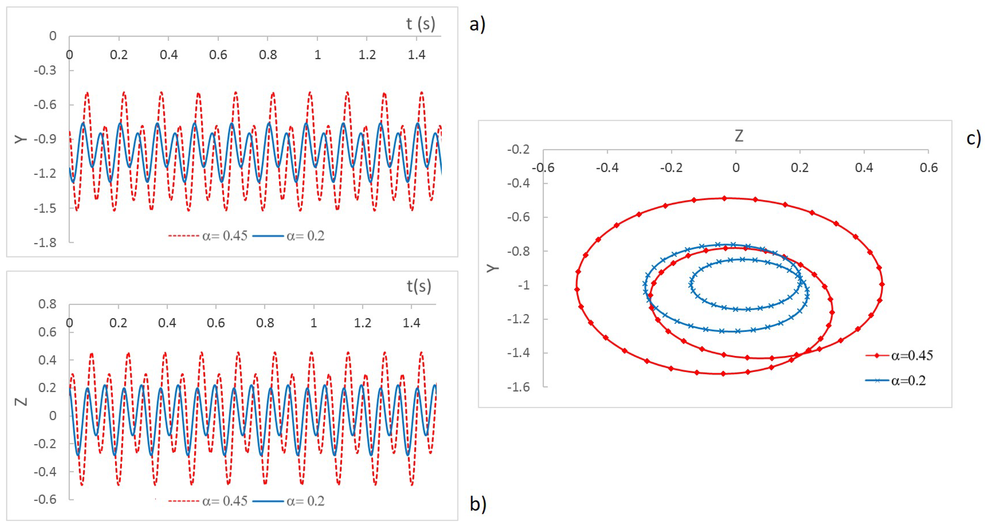
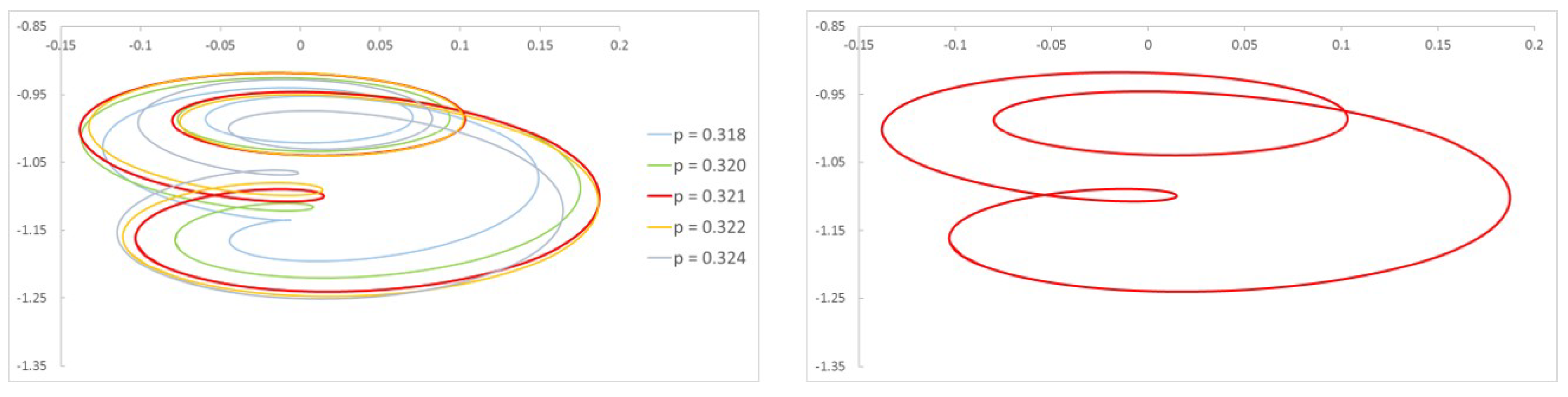
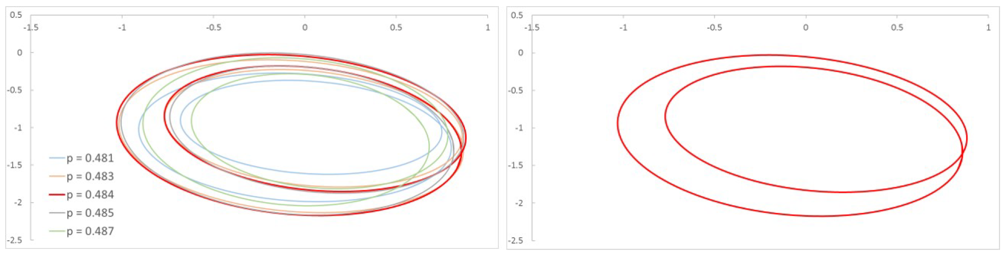
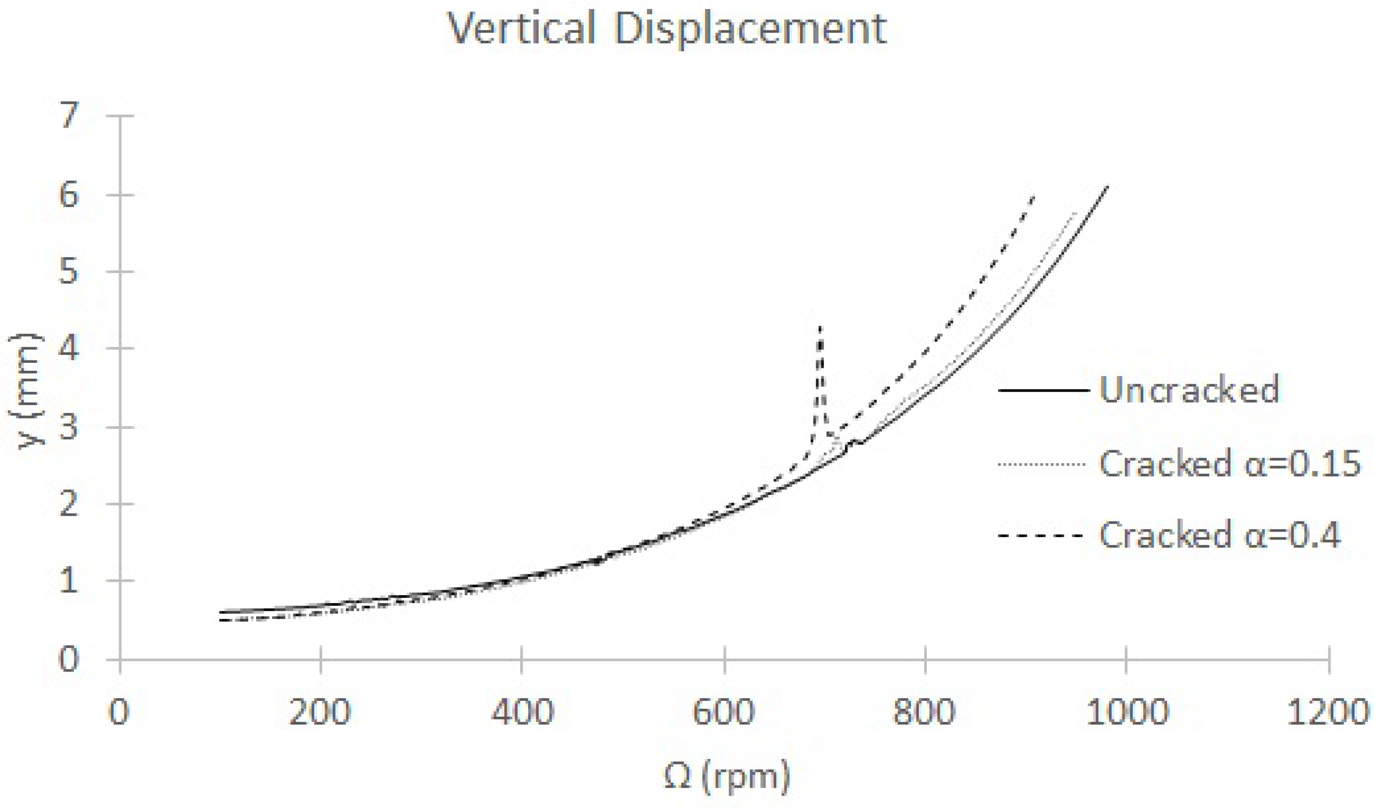
2.1. Numerical Results: Displacements and Orbits
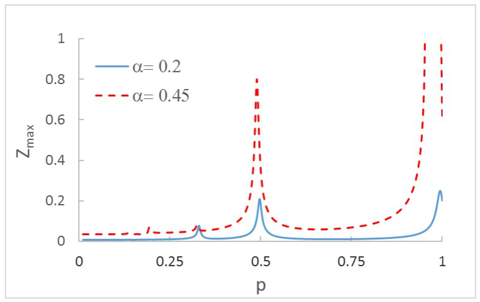
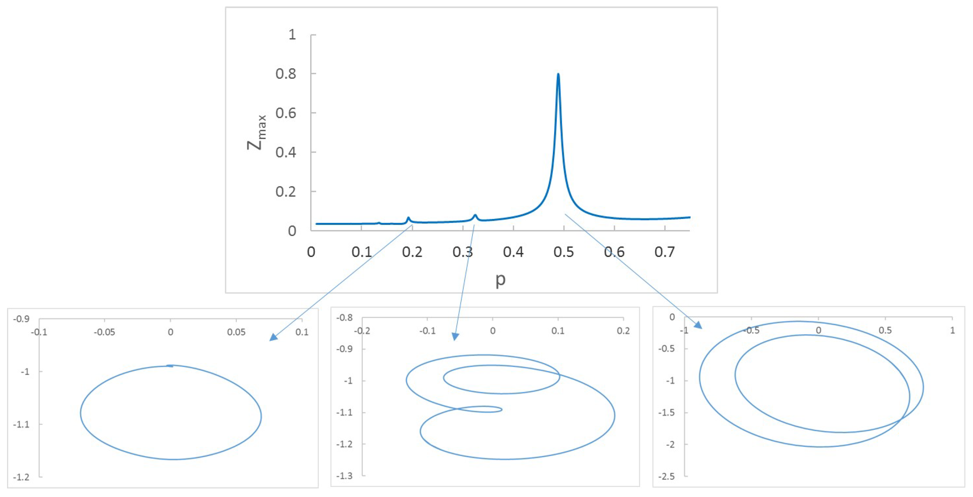
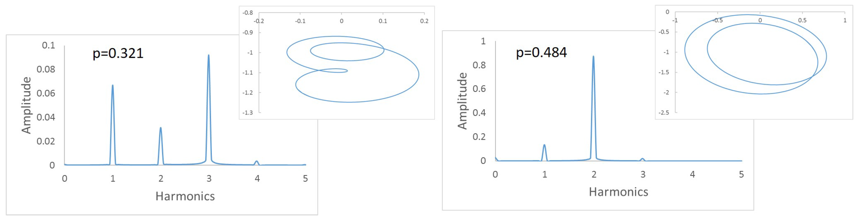
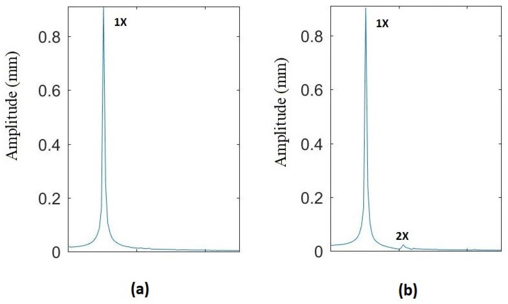
2.2. Numerical Results: Frequency Content
3. Proposed Method for Determination of the Critical Speed
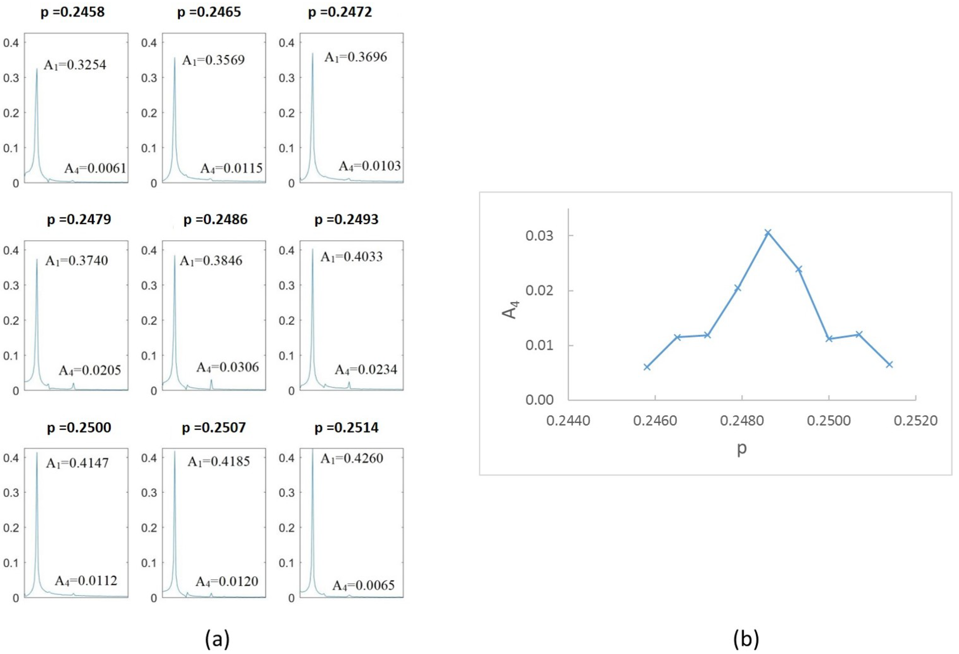
3.1. Determination of the Critical Speed
- only indicates an intact unbalanced shaft.
- only and indicate the presence of a crack. The current speed may or may not be the subcritical speed , as the two harmonics can indicate other kinds of situations that are not cracks.
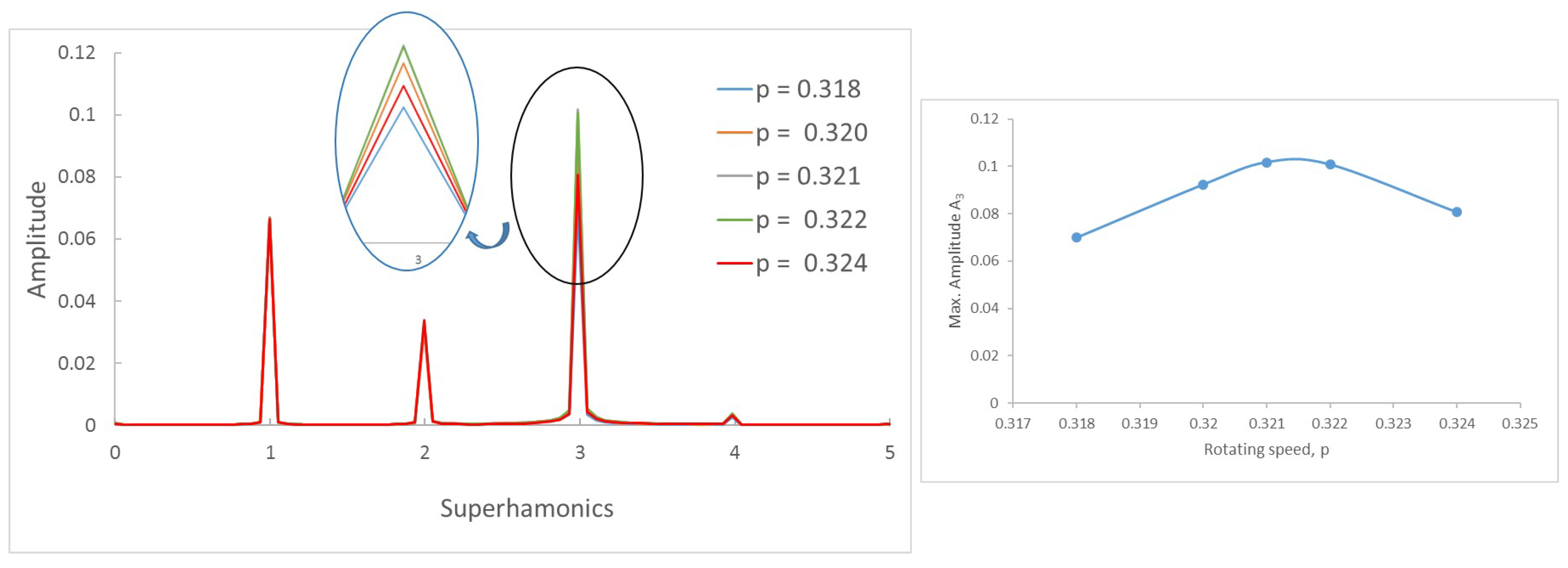
- , , ... indicates the presence of a crack and a subcritical speed
- and other harmonics , ..., while very small with respect to , indicate an intact shaft with other possible defects (i.e., clearances).
- and and other small harmonics indicate a defect (i.e., cracks or clearances). The speed may or may not be the subcritical speed , for the same reasons as before.
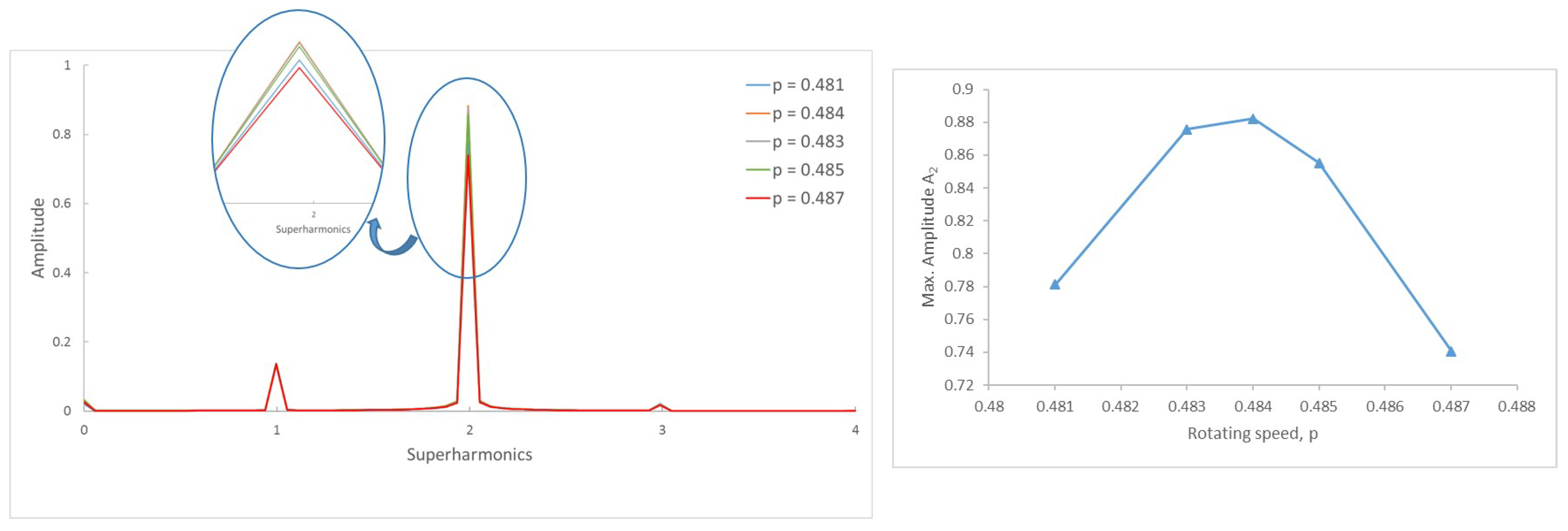
- , , ... with , , and larger than the other harmonics indicates the presence of a crack and a subcritical speed of
- , , ... with and larger than the other harmonics indicates an intact shaft and a subcritical speed of
3.2. Verification of the Method
4. Experimental Results
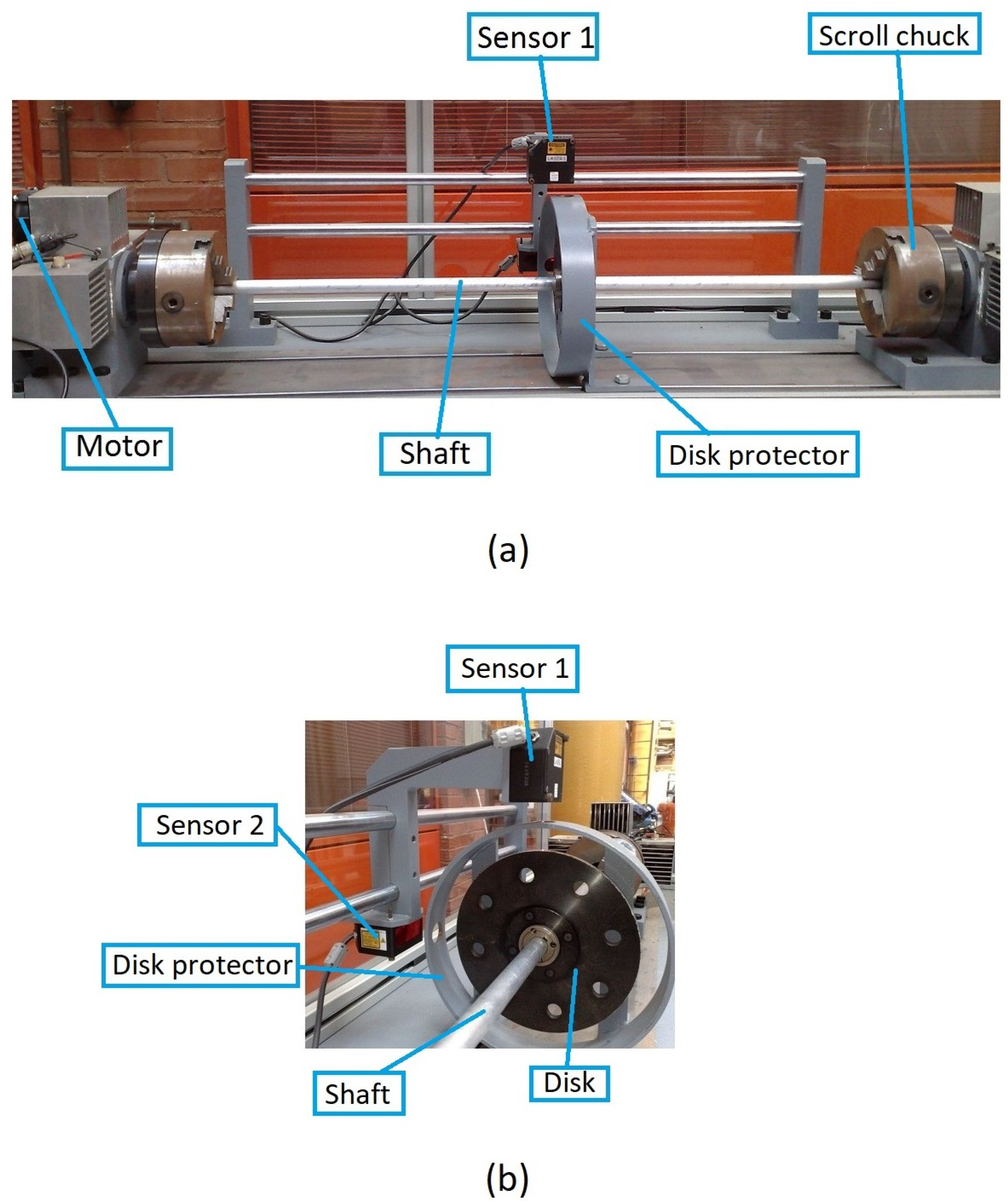
4.1. Experimental Setup
4.2. Experimental Application of the Method and Results
5. Conclusions
Author Contributions
Funding
Data Availability Statement
Conflicts of Interest
References
- Liu, J.; Tang, C.; Pan, G. Dynamic modeling and simulation of a flexible-rotor ball bearing system. J. Vib. Control. 2021, 28, 10775463211034347. [Google Scholar] [CrossRef]
- Shen, M.H.; Taylor, J.E. An identification problem for vibrating cracked beams. J. Sound Vib. 1991, 150, 457–484. [Google Scholar] [CrossRef] [Green Version]
- Narkis, Y. Identification of crack location in vibrating simply supported beams. J. Sound Vib. 1994, 172, 549–558. [Google Scholar] [CrossRef]
- Hasan, W.M. Crack detection from the variation of the eigenfrequencies of a beam on elastic foundation. Eng. Fract. Mech. 1995, 52, 409–421. [Google Scholar] [CrossRef]
- Morassi, A. Identification of a crack in a rod based on changes in a pair of natural frequencies. J. Sound Vib. 2001, 242, 577–596. [Google Scholar] [CrossRef]
- Morassi, A.; Rollo, M. Identification of two cracks in a simply supported beam from minimal frequency measurements. J. Vib. Control. 2001, 7, 729–739. [Google Scholar] [CrossRef]
- Suh, M.W.; Yu, J.M.; Lee, J.H. Crack identification using classical optimization technique. Key Eng. Mater. 2000, 183, 61–66. [Google Scholar] [CrossRef]
- Shim, M.B.; Suh, M.W. Crack identification using evolutionary algorithms in parallel computing environment. J. Sound Vib. 2003, 242, 141–160. [Google Scholar] [CrossRef]
- Dilena, M.; Morassi, A. The Use of Antiresonances for Crack Detection in Beams. J. Sound Vib. 2004, 276, 195–214. [Google Scholar] [CrossRef]
- Dong, G.M.; Chen, J.; Zou, J. Parameter identification of a rotor with an open crack. Eur. J. Mech. A/Solids 2004, 23, 325–333. [Google Scholar] [CrossRef]
- Sekhar, A.S. Model-based identification of two cracks in a rotor system. Mech. Syst. Signal Process. 2004, 18, 977–983. [Google Scholar] [CrossRef]
- Rubio, L. An Efficient Method for Crack Identification in Simply Supported Euler-Bernoulli Beams. J. Vib. Acoust. 2009, 31, 0510011. [Google Scholar] [CrossRef]
- Wauer, J. On the dynamics of cracked rotors: A literature survey. Appl. Mech. Rev. 1990, 43, 13–17. [Google Scholar] [CrossRef]
- Gasch, R. A Survey of the Dynamic Behavior of a Simple Rotating Shaft with a Transverse Crack. J. Sound Vib. 1993, 160, 313–332. [Google Scholar] [CrossRef]
- Dimarogonas, A.D. Vibration of cracked structures: A state of the art review. Eng. Fract. Mech. 1996, 55, 831–857. [Google Scholar] [CrossRef]
- Papadopoulos, C. The strain energy release approach for modeling cracks in rotors: A state of the art review. Mech. Syst. Signal Process. 2008, 22, 763–789. [Google Scholar] [CrossRef]
- Gomez-Mancilla, J.; Sinou, J.J.; Nosov, V.R.; Thouverez, F.; Zambrano, A. The influence of crack-imbalance orientation and orbital evolution for an extended cracked Jeffcott Rotor. Comptes Rendus Mec. 2004, 332, 955–962. [Google Scholar] [CrossRef] [Green Version]
- Machorro-López, J.M.; Adams, D.E.; Gómez-Mancilla, J.C.; Gul, K.A. Identification of damage shafts using active sensing-simulation and experimentation. J. Sound Vib. 2009, 327, 368–390. [Google Scholar] [CrossRef]
- Sinou, J.J. Experimental response and vibrational characteristics of a slotted rotor. Commun. Nonlinear Sci. Numer. Simul. 2009, 14, 3179–3194. [Google Scholar] [CrossRef] [Green Version]
- Sinou, J.J.; Lees, A.W. The influence of cracks in rotating shafts. J. Sound Vib. 2005, 285, 1015–1037. [Google Scholar] [CrossRef]
- Sinou, J.J. Effects of a crack on the stability of a non-linear rotor system. Int. J. Non-Linear Mech. 2007, 42, 959–972. [Google Scholar] [CrossRef] [Green Version]
- Al-Shudeifat, M.A.; Butcher, E.A. New breathing functions for the transverse breathing crack of the cracked rotorsystem: Approach for critical and subcritical harmonic analysis. J. Sound Vib. 2011, 330, 526–544. [Google Scholar] [CrossRef]
- Zhao, W.; Hua, C.; Dong, D.; Ouyang, H. A Novel Method for Identifying Crack and Shaft Misalignment Faults in Rotor Systems under Noisy Environments Based on CNN. Sensors 2019, 19, 5158. [Google Scholar] [CrossRef] [PubMed] [Green Version]
- Liang, H.; Zhao, C.; Chen, Y.; Liu, Y.; Zhao, Y. The Improved WNOFRFs Feature Extraction Method and Its Application to Quantitative Diagnosis for Cracked Rotor Systems. Sensors 2022, 22, 1936. [Google Scholar] [CrossRef] [PubMed]
- Sinou, J.J. Detection of cracks in rotor based on the 2X and 3X super-harmonic frequency components and the crack-unbalance interactions. Commun. Nonlinear Sci. Numer. Simul. 2008, 13, 2024–2040. [Google Scholar] [CrossRef] [Green Version]
- Gasch, R. Dynamic behavior of a simple rotor with a cross-sectional crack. In Proceedings of the Vibrations in Rotating Machinery, ImechE Conference Paper, Cambridge, UK, 15–17 September 1976. [Google Scholar]
- Dimarogonas, A.D.; Papadopoulos, C.A. Vibrations of cracked shafts in bending. J. Sound Vib. 1983, 91, 583–593. [Google Scholar] [CrossRef]
- Jun, O.S.; Eun, H.J.; Earmme, Y.Y.; Lee, C.W. Modelling and vibration analysis of a simple rotor with breathing crack. J. Sound Vib. 1992, 155, 273–290. [Google Scholar] [CrossRef]
- Penny, J.E.T.; Friswell, M.I. Simplified modelling of rotor cracks. In Proceedings of the ISMA: International Conference on Noise and Vibration Engineering, Leuven, Belgium, 16–18 September 2002; Volume 2, pp. 607–615. [Google Scholar]
- Darpe, A.K.; Gupta, K.; Chawla, A. Transient response and breathing behaviour of a cracked Jeffcott Rotor. J. Sound Vib. 2004, 272, 207–243. [Google Scholar] [CrossRef]
- Patel, T.H.; Darpe, A. Influence of crack breathing model on nonlinear dynamics of a cracked rotor. J. Sound Vib. 2008, 311, 953–972. [Google Scholar] [CrossRef]
- Papadopoulos, C.A.; Dimarogonas, A.D. Coupled longitudinal and bending vibrations of a rotating shaft with an open crack. J. Sound Vib. 1987, 117, 81–93. [Google Scholar] [CrossRef]
- Qin, W.Y.; Meng, G.; Zhang, T. The swing vibration, transverse oscillation of cracked rotor and the itermittence chaos. J. Sound Vib. 2003, 259, 571–583. [Google Scholar] [CrossRef]
- Müller, P.C.; Bajkowski, J.; Söffker, D. Chaotic motions and fault detection in a cracked rotor. Nonlinear Dyn. 1994, 5, 233–254. [Google Scholar] [CrossRef]
- Pu, Y.; Chen, J.; Zou, J.; Zhong, P. Quasi-periodic vibration of cracked rotor on flexible bearings. J. Sound Vib. 2002, 251, 875–890. [Google Scholar] [CrossRef]
- Gasch, R. Dynamic behaviour of the Laval rotor with a transverse crack. Mech. Syst. Signal Process. 2008, 22, 790–804. [Google Scholar] [CrossRef]
- Papadopoulos, C.A. Some comments on the calculation of the local flexibility of cracked shafts. J. Sound Vib. 2004, 278, 1205–1211. [Google Scholar] [CrossRef]
- Rubio, L.; Fernández-Sáez, J. A new efficient procedure to solve the nonlinear dynamics of a cracked rotor. Nonlinear Dyn. 2012, 70, 1731–1745. [Google Scholar] [CrossRef]
- Chan, R.K.C.; Lai, T.C. Digital simulation of a rotating shaft with a transverse crack. Appl. Math. Model. 1995, 19, 411–420. [Google Scholar] [CrossRef]
- Rodríguez, C.; Steffen, V. Diagnosis of cracked shafts by monitoring the transient motion response. In Proceedings of the XII International Symposium on Dynamic Problems of Mechanics (2007), Ibiza, Spain, 21–23 May 2007. [Google Scholar]
- Virgin, L.N.; Knight, J.D.; Plaut, R.H. A New Method for Predicting Critical Speeds in Rotordynamics. J. Eng. Gas Turbines Power 2015, 138, 022504. [Google Scholar] [CrossRef]
- Guo, C.; Yan, J.; Yang, W. Crack detection for a Jeffcott Rotor with a transverse crack: An experimental investigation. Mech. Syst. Signal Process. 2017, 83, 260–271. [Google Scholar] [CrossRef]
- ElArem, S.; Zid, M.B. On a systematic approach for cracked rotating shaft study: Breathing mechanism, dynamics and instability. Nonlinear Dyn. 2017, 88, 2123–2138. [Google Scholar] [CrossRef]
- Muszynska, A. Misalignment and Shaft Crack-Related Phase Relationships for 1X and 2X Vibration Components of Rotor Responses. Orbit 1989, 10, 4–8. [Google Scholar]
- Guo, C.; AL-Shudeifat, M.A.; Yana, J.; Bergman, L.A.; McFarland, D.M.; Butcher, E.A. Application of empirical mode decomposition to a Jeffcott Rotor with a breathing crack. J. Sound Vib. 2013, 332, 3881–3892. [Google Scholar] [CrossRef]
- Goldman, P.; Muszynska, A. Application of full spectrum to rotating machinery diagnostics. Orbit 1999, 20, 17–21. [Google Scholar]
- Varney, P.; Green, I. Rotordynamic Crack Diagnosis: Distinguishing Crack Depth and Location. J. Eng. Gas Turbines Power 2013, 135, 112101. [Google Scholar] [CrossRef]
- Ansari, A.I.; Chauhan, S.J.; Khaire, P. Effect of Crack on Natural Frecuency in Rotor System. In Proceedings of the International Conference on FCSPTC 2017, Andhrapradesh, India, 7–8 April 2017. [Google Scholar]
- Ehrich, F. Observations of Subcritical Superharmonic and Chaotic Response in Rotordynamics. J. Vib. Acoust. 1992, 114, 93–100. [Google Scholar] [CrossRef]
- Sabnavis, G.; Kirk, R.G.; Kasarda, M.; Quinn, D. Cracked Shaft Detection and Diagnostics: A Literature Review. Shock Vib. Dig. 2004, 36, 287. [Google Scholar] [CrossRef]
- Pirogova, N.; Taranenko, P. Calculative and experimental analysis of natural and critical frequencies and mode shapes of high-speed rotor for micro gas turbine plant. Procedia Eng. 2015, 129, 997–1004. [Google Scholar] [CrossRef] [Green Version]
- Gayen, D.; Chakraborty, D.; Tiwari, R. Whirl frequencies and critical speeds of a rotor-bearing system with a cracked functionally graded shaft-Finite element analysis. Eur. J. Mech. A/Solids 2017, 61, 47–51. [Google Scholar] [CrossRef]
- White, R.J. Measurement Techniques for Estimating Critical Speed of Drivelines. Sound Vib. 2017, 51, 10–15. [Google Scholar]
- Montero, L. Estudio Numérico y Experimental de un eje Giratorio Fisurado Determinación del Factor de Intensidad de Tensiones. Doctoral Thesis, Universidad Carlos III de Madrid, Getafe, Spain, 2017. [Google Scholar]


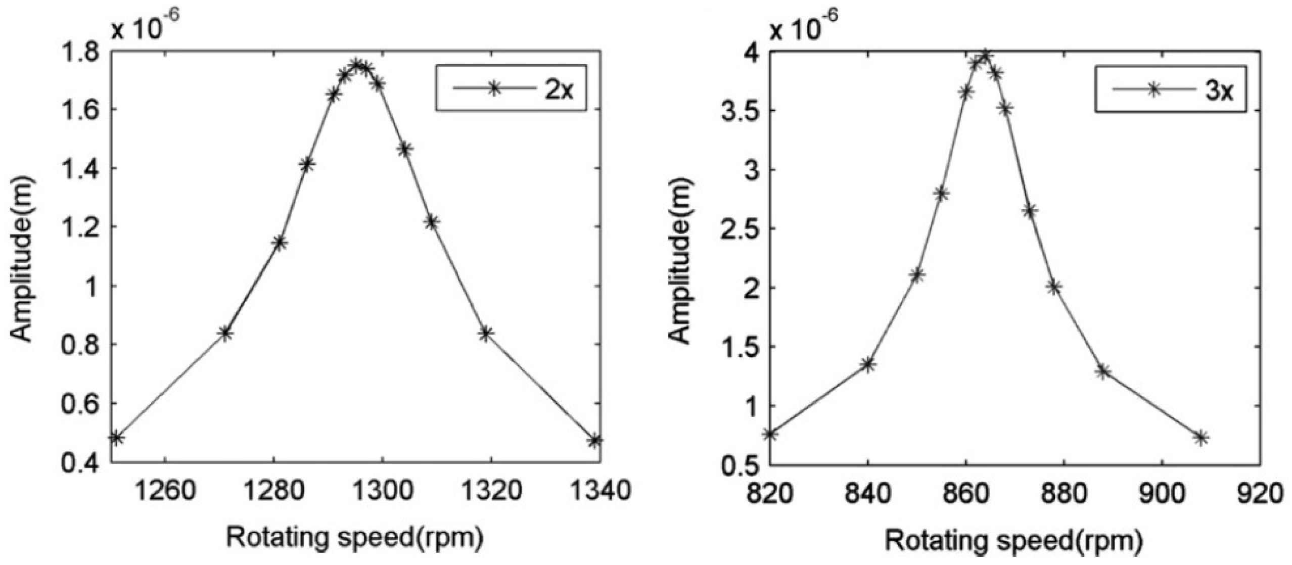
| (rpm) | Amplitude of 2X |
|---|---|
| 1271.18 | 0.84 × |
| 1281.18 | 1.17 × |
| 1286.47 | 1.43 × |
| 1291.17 | 1.76 × |
| 1295.29 | 1.79 × |
| 1297.06 | 1.77 × |
| 1299.41 | 1.72 × |
| 1304.71 | 1.48 × |
| 1309.41 | 1.24 × |
| (rpm) | Amplitude of 3X |
|---|---|
| 850.15 | 2.08 × |
| 855.06 | 2.75 × |
| 859.98 | 3.63 × |
| 861.82 | 3.83 × |
| 864.28 | 3.90 × |
| 866.13 | 3.75 × |
| 867.97 | 3.48 × |
| 872.89 | 2.60 × |
| 878.43 | 1.98 × |
| From | rpm | rpm | rpm |
|---|---|---|---|
| Horizontal displacement | 1440 | 1464 | 1470 |
| Vertical displacement | 1432 | 1455 | 1456 |
Publisher’s Note: MDPI stays neutral with regard to jurisdictional claims in published maps and institutional affiliations. |
© 2022 by the authors. Licensee MDPI, Basel, Switzerland. This article is an open access article distributed under the terms and conditions of the Creative Commons Attribution (CC BY) license (https://creativecommons.org/licenses/by/4.0/).
Share and Cite
Muñoz-Abella, B.; Montero, L.; Rubio, P.; Rubio, L. Determination of the Critical Speed of a Cracked Shaft from Experimental Data. Sensors 2022, 22, 9777. https://doi.org/10.3390/s22249777
Muñoz-Abella B, Montero L, Rubio P, Rubio L. Determination of the Critical Speed of a Cracked Shaft from Experimental Data. Sensors. 2022; 22(24):9777. https://doi.org/10.3390/s22249777
Chicago/Turabian StyleMuñoz-Abella, Belén, Laura Montero, Patricia Rubio, and Lourdes Rubio. 2022. "Determination of the Critical Speed of a Cracked Shaft from Experimental Data" Sensors 22, no. 24: 9777. https://doi.org/10.3390/s22249777
APA StyleMuñoz-Abella, B., Montero, L., Rubio, P., & Rubio, L. (2022). Determination of the Critical Speed of a Cracked Shaft from Experimental Data. Sensors, 22(24), 9777. https://doi.org/10.3390/s22249777