
Classification of Gravity Matching Areas Using PSO-BP Neural Networks based on PCA and Satellite Altimetry Data over the Western Pacific

Abstract
:1. Introduction
2. Methods
2.1. Gravity Characteristic Selection Method
- 1.
- Standard deviation of gravity anomaly ():
- 2.
- Standard deviation of slope ():
- 3.
- Roughness of gravity anomaly ():
- 4.
- Relevant coefficient ():
- 5.
- Average gravity difference ():
- 6.
- Fractal dimension ():
- 7.
- Kurtosis coefficient ():
2.2. The Proposed Principal-Component-Analysis-Based Method
- (1)
- Start;
- (2)
- Step (1) Select characteristic parameter ;
- (3)
- Step (2) Standardize X and compute its covariance matrix;
- (4)
- Step (3) Calculate the eigenvalues and eigenvectors of the covariance matrix;
- (5)
- Step (4) Calculate the PCA expression and the new principal component index;
- (6)
- End.
2.3. The PSO-BP Combined Artificial Neural Network Algorithm
2.3.1. BP NN
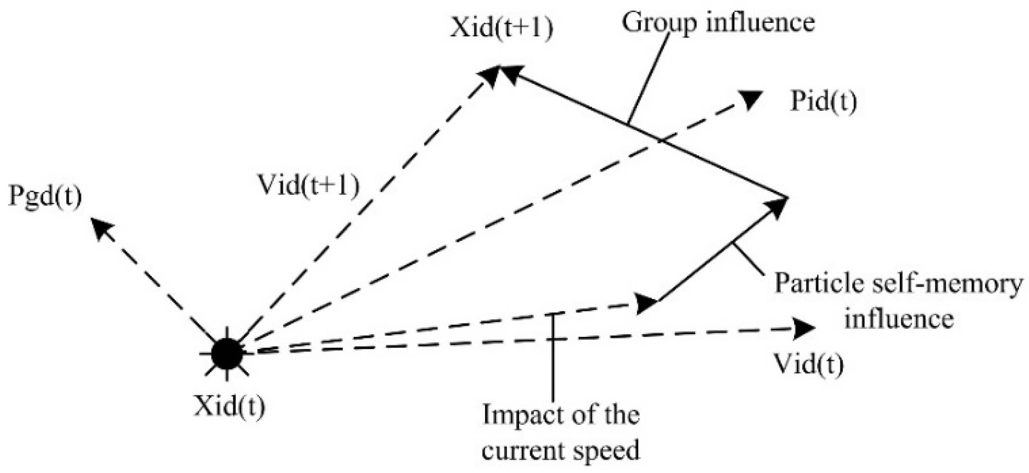
2.3.2. PSO
2.4. The PCA-PSO-BP Combined Algorithm Method
3. Materials
4. Experiments and Results
4.1. Characteristic Parameters of the Gravity Field in the Experiment Region
4.2. Results of the PPBA Method and the Classification Evaluation Index
- Accuracy (A):
- Precision-T (PT):
- Precision-F (PF):
- Average classification accuracy (AA):
4.3. Classification Results by PPBA
5. Discussion
6. Conclusions
Author Contributions
Funding
Data Availability Statement
Acknowledgments
Conflicts of Interest
Abbreviations
| Accuracy | A |
| average classification accuracy | AA |
| Artificial neural networks | ANN |
| Ant Colony Optimization | ACO |
| Artificial Bee Colony | ABC |
| back propagation | BP |
| Differential Evolution | DE |
| Fractal theory | FD |
| Genetic Algorithm | GA |
| Grey Wolf Optimizer | GWO |
| Inertial navigation systems | INS |
| matching probability | MP |
| Multi-Layer Perceptron | MLP |
| neural networks | NN |
| Precision-T | PT |
| Precision-F | PF |
| particle swarm optimization | PSO |
| principal component analysis | PCA |
| PCA theory and PSO-BP neural networks | PPBA |
| Terrain Contour Matching | TERCOM |
| sine-cosine algorithm | SCA |
References
- Wang, B.; Ren, Q.; Deng, Z.; Fu, M. A self-calibration method for nonorthogonal angles between gimbals of rotational inertial navigation system. IEEE Trans. Ind. Electron. 2015, 62, 2353–2362. [Google Scholar] [CrossRef]
- Wang, C.; Deng, Z.; Fu, M. A delaunay triangulation based matching area selection algorithm for underwater gravity-aided inertial navigation. IEEE/ASME Trans. Mechatron. 2020, 26, 908–917. [Google Scholar] [CrossRef]
- Plueddemann, A.; Kukulya, A.; Stokey, R.; Freitag, L. Autonomous underwater vehicle operations beneath coastal sea ice. IEEE-ASME Trans. Mechatron. 2012, 17, 54–64. [Google Scholar] [CrossRef]
- Andersen, O.B.; Knudsen, P.; Trimmer, R.G. Improved high resolution altimetric gravity field mapping (KMS2002 global marine gravity field). In International Association of Geodesy Symposia; Ramillien, G., Cazenave, A., Reigber, C., Schmidt, R., Schwintzer, P., Eds.; Springer-Verlag Inc.: New York, NY, USA, 2004; Volume 128, pp. 326–331. [Google Scholar]
- Sandwell, D. Antarctic marine gravity field from high-density satellite altimetry. Geophys. J. Int. 1992, 109, 437–448. [Google Scholar] [CrossRef] [Green Version]
- Panahandeh, G.; Jansson, M. Vision-aided inertial navigation based on ground plane feature detection. IEEE/ASME Trans. Mechatron. 2014, 19, 1206–1215. [Google Scholar] [CrossRef]
- Zhao, L.; Gao, N.; Huang, B.; Wang, Q.; Zhou, J. A novel terrain-aided navigation algorithm combined with the TERCOM algorithm and particle filter. IEEE Sens. J. 2015, 15, 1124–1131. [Google Scholar] [CrossRef]
- Peng, C. Straight-line geomagnetic matching for underwater base on ICCP. J. Chin. Inert. Technol. 2009, 17, 153–155. [Google Scholar]
- Adamek, T.; Kitts, C.; Mas, I. Gradient-based cluster space navigation for autonomous surface vessels. IEEE/ASME Trans. Mechatron. 2015, 20, 506–518. [Google Scholar] [CrossRef]
- Arquero, A.; Alvarez, M.; Martinez, E. Decision management making by AHP (Analytical Hierarchy Process) trought GIS data. IEEE Lat. Am. Trans. 2009, 7, 101–106. [Google Scholar] [CrossRef]
- Pedrycz, W.; Song, M. Analytic Hierarchy Process (AHP) in group decision making and its optimization with an allocation of information granularity. IEEE Trans. Fuzzy Syst. 2011, 19, 527–539. [Google Scholar] [CrossRef]
- Li, Z.; Zheng, W.; Fang, J.; Wu, F. Optimizing suitability area of underwater gravity matching navigation based on a new principal component weighted average normalization method. Chin. J. Geophys. 2019, 62, 3269–3278. [Google Scholar]
- Wang, H.; Wu, L.; Chai, H.; Xiao, Y.; Hsu, H.; Wang, Y. Characteristics of marine gravity anomaly reference maps and accuracy analysis of gravity matching-aided navigation. Sensors 2017, 17, 1851. [Google Scholar] [CrossRef] [PubMed]
- Zitová, B.; Flusser, J. Image registration methods: A survey. Image Vis. Comput. 2003, 21, 977–1000. [Google Scholar] [CrossRef] [Green Version]
- Goldenberg, F. Geomagnetic navigation beyond the magnetic compass. In Proceedings of the 2006 IEEE/ION Position, Location, and Navigation Symposium, Coronado, CA, USA, 25–27 April 2006; pp. 684–694. [Google Scholar]
- Potlapalli, H.; Luo, R.C. Fractal-based classification of natural textures. IEEE Trans. Ind. Electron. 1998, 45, 142–150. [Google Scholar] [CrossRef]
- Shukla, R.K.; Giri, P. Isotropic finite volume discretization. J. Comput. Phys. 2014, 276, 252–290. [Google Scholar] [CrossRef]
- Butera, S.; Di Paola, M. A physically based connection between fractional calculus and fractal geometry. Ann. Phys. 2014, 350, 146–158. [Google Scholar] [CrossRef] [Green Version]
- Zhu, Y.; Zhihong, D.; Fu, M. The gravity matching area selection criteria for underwater gravity aided navigation application based on the comprehensive characteristic parameter. IEEE/ASME Trans. Mechatron. 2016, 21, 2935–2943. [Google Scholar] [CrossRef]
- Chan, L.W.; Fallside, F. An adaptive training algorithm for back propagation networks. Comput. Speech Lang. 1987, 2, 205–218. [Google Scholar] [CrossRef]
- Rumelhart, D.E.; McClelland, J.L.; PDP Research Group. Parallel Distributed Processing: Explorations in the Microstructure of Cognition: Foundations; MIT Press: Cambridge, MA, USA, 1986. [Google Scholar] [CrossRef] [Green Version]
- Sundermeyer, M.; Ney, H.; Schlüter, R. From feedforward to recurrent LSTM neural networks for language modeling. IEEE/ACM Trans. Audio Speech Lang. Process. 2015, 23, 517–529. [Google Scholar] [CrossRef]
- Phansalkar, V.V.; Sastry, P.S. Analysis of the back-propagation algorithm with momentum. IEEE Trans. Neural Netw. 1994, 5, 505–506. [Google Scholar] [CrossRef] [Green Version]
- Meybodi, M.R.; Beigy, H. A note on learning automata-based schemes for adaptation of BP parameters. Neurocomputing 2002, 48, 957–974. [Google Scholar] [CrossRef]
- Bhaya, A.; Kaszkurewicz, E. Steepest descent with momentum for quadratic functions is a version of the conjugate gradient method. Neural Netw. Off. J. Int. Neural Netw. Soc. 2004, 17, 65–71. [Google Scholar] [CrossRef] [PubMed] [Green Version]
- Hager, W.W.; Zhang, H. A new conjugate gradient method with guaranteed descent and an efficient line search. SIAM J. Optim. 2005, 16, 170–192. [Google Scholar] [CrossRef] [Green Version]
- Nocedal, J.; Wright, S.J. Numerical Optimization; Springer: New York, NY, USA, 1999; pp. 21–25. [Google Scholar]
- Zhao, Y.; Juang, B.H. Nonlinear compensation using the Gauss–Newton method for noise-robust speech recognition. IEEE Trans. Audio Speech Lang. Process. 2012, 20, 2191–2206. [Google Scholar] [CrossRef]
- Podlena, J.R.; Hendtlass, T. An accelerated genetic algorithm. Appl. Intell. 1998, 8, 103–111. [Google Scholar] [CrossRef]
- Mirjalili, S.; Mohd Hashim, S.Z.; Moradian Sardroudi, H. Training feedforward neural networks using hybrid particle swarm optimization and gravitational search algorithm. Appl. Math. Comput. 2012, 218, 11125–11137. [Google Scholar] [CrossRef]
- Kennedy, J.; Eberhart, R. Particle swarm optimization. In Proceedings of the ICNN’95—International Conference on Neural Networks, Perth, WA, Australia, 27 November–1 December 1995; Volume 1944, pp. 1942–1948. [Google Scholar]
- Spears, W.; Green, D.; Spears, D. Biases in particle swarm optimization. IJSIR 2010, 1, 34–57. [Google Scholar] [CrossRef]
- Altınöz, T.; Tanyer, S.G.; Yilmaz, A. A comparative study of fuzzy-PSO and chaos-PSO. Electroteh. Versnik 2012, 79, 68–72. [Google Scholar]
- Socha, K.; Blum, C. An ant colony optimization algorithm for continuous optimization: Application to feed-forward neural network training. Neural Comput. Appl. 2007, 16, 235–247. [Google Scholar] [CrossRef]
- Karaboga, D.; Akay, B.; Ozturk, C. Artificial Bee Colony (ABC) Optimization algorithm for training feed-forward neural networks. In Proceedings of the Modeling Decisions for Artificial Intelligence, Berlin/Heidelberg, Germany, 16–18 August 2007; pp. 318–329. [Google Scholar]
- Ozturk, C.; Karaboga, D. Hybrid Artificial Bee Colony algorithm for neural network training. In Proceedings of the 2011 IEEE Congress of Evolutionary Computation (CEC), Wellington, New Zealand, 5–8 June 2011; pp. 84–88. [Google Scholar]
- Slowik, A.; Bialko, M. Training of artificial neural networks using differential evolution algorithm. In Proceedings of the 2008 Conference on Human System Interactions, Krakow, Poland, 25–27 May 2008; pp. 60–65. [Google Scholar]
- Wang, Y.; Peng, H. Underwater acoustic source localization using generalized regression neural network. J. Acoust. Soc. Am. 2018, 143, 2321. [Google Scholar] [CrossRef]
- Mirjalili, S. How effective is the Grey Wolf optimizer in training multi-layer perceptrons. Appl. Intell. 2015, 43, 150–161. [Google Scholar] [CrossRef]
- Hosseini Nejad Takhti, A.; Saffari, A.; Martín, D.; Khishe, M.; Mohammadi, M. Classification of marine mammals using the trained multilayer perceptron neural network with the whale algorithm developed with the fuzzy system. Comput. Intell. Neurosci. 2022, 2022, 3216400. [Google Scholar] [CrossRef] [PubMed]
- Saffari, A.; Khishe, M.; Zahiri, S.-H. Fuzzy-ChOA: An improved chimp optimization algorithm for marine mammal classification using artificial neural network. Analog. Integr. Circuits Signal Process. 2022, 111, 403–417. [Google Scholar] [CrossRef] [PubMed]
- Wang, Y.; Yuan, L.; Khishe, M.; Moridi, A.; Mohammadzade, F. Training RBF NN Using sine-cosine algorithm for sonar target classification. Arch. Acoust. 2020, 45, 753–764. [Google Scholar]
- Ma, Y.Y.; Ouyang, Y.Z.; Huang, M.T.; Deng, K.L.; Qu, Z.H. Selection method for gravity-field matchable area based on information entropy of characteristic parameters. J. China Inert. Technol. 2016, 24, 763–768. [Google Scholar] [CrossRef]
- Majhi, B.R. Gravitational anomalies and entropy. Gen. Relativ. Gravit. 2013, 45, 345–357. [Google Scholar] [CrossRef] [Green Version]
- Wu, L.; Wang, H.; Chai, H.; Zhang, L.; Hsu, H.; Wang, Y. Performance evaluation and analysis for gravity matching aided navigation. Sensors 2017, 17, 769. [Google Scholar] [CrossRef] [Green Version]
- Sarkar, N.; Chaudhuri, B.B. An efficient differential box-counting approach to compute fractal dimension of image. IEEE Trans. Syst. Man Cybern. 1994, 24, 115–120. [Google Scholar] [CrossRef] [Green Version]
- Rumelhart, D.E.; Hinton, G.E.; Williams, R.J. Learning representations by back-propagating errors. Nature 1986, 323, 533–536. [Google Scholar] [CrossRef]
- Krasnov, A.A.; Nesenyuk, L.P.; Peshekhonov, V.G.; Sokolov, A.V.; Elinson, L.S. Integrated marine gravimetric system. Development and operation results. Gyroscopy Navig. 2011, 2, 75–81. [Google Scholar] [CrossRef]
- Sandwell, D.; Garcia, E.; Soofi, K.; Wessel, P.; Hamilton, M.; Smith, W. Toward 1-mGal accuracy in global marine gravity from CryoSat-2, Envisat, and Jason-1. Lead. Edge 2013, 32, 892–899. [Google Scholar] [CrossRef] [Green Version]
- Sandwell, D.; Müller, D.; Smith, W.; Garcia, E.; Francis, R. New global marine gravity from CryoSat-2 and Jason-1 reveals buried tectonic structure. Science 2014, 346, 65–67. [Google Scholar] [CrossRef] [PubMed]
- Krasnov, A.A.; Sokolov, A.V.; Elinson, L.S. Operational experience with the Chekan-AM gravimeters. Gyroscopy Navig. 2014, 5, 181–185. [Google Scholar] [CrossRef]
- Yu-De, T.; Shao-Feng, B.; Dong-Fang, J.; Cai-Bing, X. A new integrated gravity matching algorithm based on approximated local gravity map. Chin. J. Geophys. 2012, 55, 2917–2924. [Google Scholar] [CrossRef]
- Gupta, D.; Kose, U.; Khanna, A.; Balas, V.E. Deep Learning for Medical Applications with Unique Data; Academic Press: Washington, DC, USA, 2022; pp. 31–51. ISBN 9780128241455. [Google Scholar] [CrossRef]
- Bazi, Y.; Melgani, F. Toward an optimal SVM classification system for hyperspectral remote sensing images. IEEE Trans. Geosci. Remote Sens. 2006, 44, 3374–3385. [Google Scholar] [CrossRef]


| Characteristic Parameters of the Gravity Field | Feature Description | Correlation with Gravity Anomaly |
|---|---|---|
| σ | overall variation characteristics of the gravity field | Positive |
| characteristics of the rate of slope change | Positive | |
| R | smoothness of the trend surface of the gravity field | Positive |
| H | the amount of information in gravity field | Negative |
| RC | relevant between neighboring grid in gravity field | Negative |
| AG | degree of the gravity changes in regions or regions | Positive |
| FD | complex irregularity shape of the local gravity field | Positive |
| PK | sharpness and flatness of the gravity anomaly distribution | Positive |
| Principal Component | Eigenvalues | Variance Contribution Rate/% | Cumulative Contribution Rate/% |
|---|---|---|---|
| First | 4.0702 | 50.877 | 50.877 |
| Second | 1.4717 | 19.396 | 69.273 |
| Third | 1.0117 | 12.646 | 82.919 |
| Fourth | 0.5169 | 6.861 | 89.780 |
| Fifth | 0.4535 | 5.669 | 95.449 |
| Sixth | 0.2900 | 2.226 | 97.675 |
| Seventh | 0.1509 | 1.887 | 99.562 |
| Eighth | 0.0350 | 0.438 | 100.000 |
| Characteristic Parameters of the Gravity Field | First Component | Second Component | Third Component | Fourth Component | Fifth Component |
|---|---|---|---|---|---|
| σ | 0.94166 | −0.04244 | −0.05438 | −0.10338 | 0.17976 |
| 0.89217 | 0.14041 | 0.07922 | 0.03174 | 0.26915 | |
| R | 0.94146 | −0.01915 | 0.05935 | −0.05234 | 0.22774 |
| H | −0.23897 | 0.83033 | 0.09734 | 0.46948 | 0.13206 |
| RR | −0.80304 | −0.09542 | −0.23105 | −0.08109 | 0.45517 |
| AG | 0.32659 | −0.77711 | −0.09100 | 0.52420 | −0.00958 |
| FD | −0.81539 | −0.34302 | 0.05911 | 0.01189 | 0.26346 |
| PK | −0.16612 | −0.17225 | 0.96141 | −0.02337 | 0.05284 |
| Prediction | |||
| Reference | Positive | Negative | |
| Positive | Ture Positive | False Negative | |
| Negative | False Positive | Ture Negative | |
| Test | PT/% | PF/% | A/% | AA/% |
|---|---|---|---|---|
| 1 | 92.00 | 83.19 | 87.00 | 87.60 |
| 2 | 87.50 | 93.97 | 91.25 | 90.74 |
| 3 | 85.71 | 99.14 | 93.50 | 92.43 |
| 4 | 92.86 | 99.57 | 96.75 | 96.22 |
| Region | Matching Probability/% | Category Labels |
|---|---|---|
| Region-A | 92.25 | suitable |
| Region-B | 89.50 | suitable |
| Region-C | 47.06 | unsuitable |
| Region-D | 65.31 | unsuitable |
| Region | Direction | Max | Min | Mean | Std |
|---|---|---|---|---|---|
| Latitude | 0.0569 | 0.0563 | 0.0566 | 0.0002 | |
| Region-A | Longitude | 0.14547 | 0.0004 | 0.0607 | 0.0422 |
| Radial | 0.1560 | 0.0567 | 0.0881 | 0.0303 | |
| Latitude | 0.2183 | 0.0005 | 0.0932 | 0.0598 | |
| Region-B | Longitude | 0.0217 | 0.0201 | 0.0209 | 0.0005 |
| Radial | 0.2190 | 0.0211 | 0.0972 | 0.0567 | |
| Latitude | 11.708 | 0.0157 | 4.9348 | 3.4992 | |
| Region-C | Longitude | 6.1323 | 2.7586 | 4.4446 | 0.9890 |
| Radial | 13.217 | 3.4531 | 6.8902 | 3.1339 | |
| Latitude | 1.5691 | 0.5825 | 1.0758 | 0.2891 | |
| Region-D | Longitude | 6.2376 | 0.0414 | 2.6116 | 1.8381 |
| Radial | 6.4319 | 0.8289 | 2.8950 | 1.7479 |
Publisher’s Note: MDPI stays neutral with regard to jurisdictional claims in published maps and institutional affiliations. |
© 2022 by the authors. Licensee MDPI, Basel, Switzerland. This article is an open access article distributed under the terms and conditions of the Creative Commons Attribution (CC BY) license (https://creativecommons.org/licenses/by/4.0/).
Share and Cite
Zong, J.; Bian, S.; Tong, Y.; Ji, B.; Li, H.; Xi, M. Classification of Gravity Matching Areas Using PSO-BP Neural Networks based on PCA and Satellite Altimetry Data over the Western Pacific. Sensors 2022, 22, 9892. https://doi.org/10.3390/s22249892
Zong J, Bian S, Tong Y, Ji B, Li H, Xi M. Classification of Gravity Matching Areas Using PSO-BP Neural Networks based on PCA and Satellite Altimetry Data over the Western Pacific. Sensors. 2022; 22(24):9892. https://doi.org/10.3390/s22249892
Chicago/Turabian StyleZong, Jingwen, Shaofeng Bian, Yude Tong, Bing Ji, Houpu Li, and Menghan Xi. 2022. "Classification of Gravity Matching Areas Using PSO-BP Neural Networks based on PCA and Satellite Altimetry Data over the Western Pacific" Sensors 22, no. 24: 9892. https://doi.org/10.3390/s22249892