
Condition Monitoring of Railway Crossing Geometry via Measured and Simulated Track Responses

 ,
,  ,
,
Abstract
:1. Introduction
2. Measurement Data
2.1. Crossing Rail Geometry Scans
2.1.1. Processing of Crossing Rail Geometry Scans
- Detection and removal of outlying data points with a fine point distance tolerance for meshing surfaces.
- Orienting the geometry in space to the defined reference frame of the MBS.
- Interpolation of cloud point data to a specified horizontal grid (nearest-neighbor method [20], 0.1-mm horizontal and 1-mm longitudinal spacing).
- Smoothening of the data with two decoupled moving average filters (2-mm lateral and 20-mm longitudinal filter length).
- Sampling the data to 2D profiles with a specified longitudinal spacing (chosen longitudinal spacing: 10 mm).
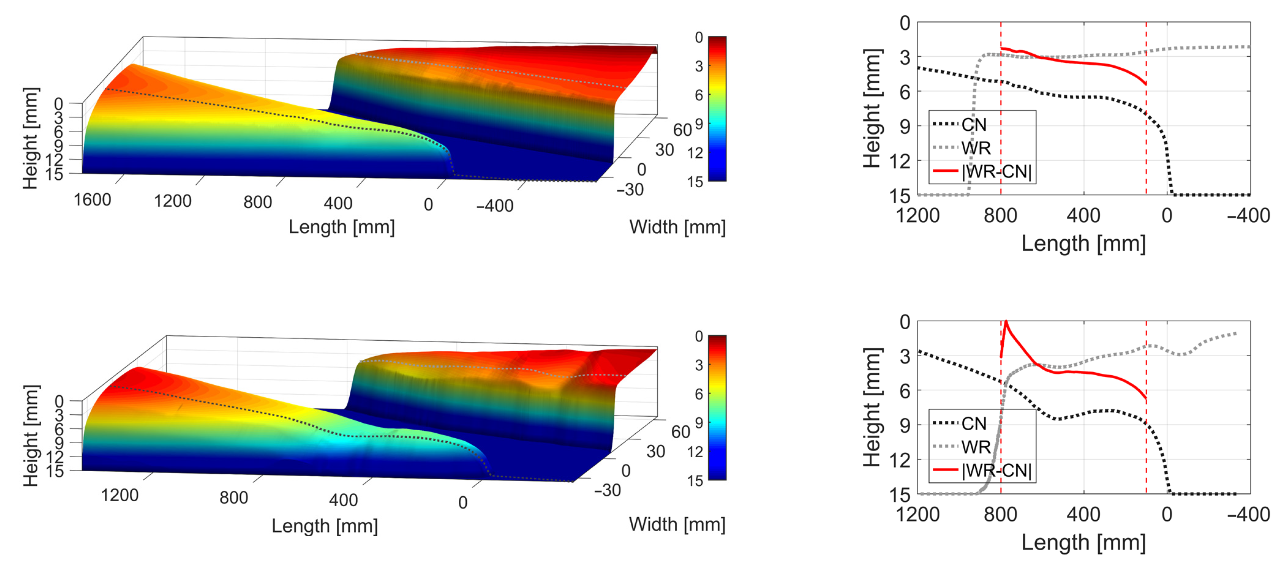
2.1.2. Post-Processed Crossing Rail Geometries
2.2. Sleeper Acceleration Measurements
3. Model for Simulation of Dynamic Train–Track Interaction
3.1. Sleeper Void Model
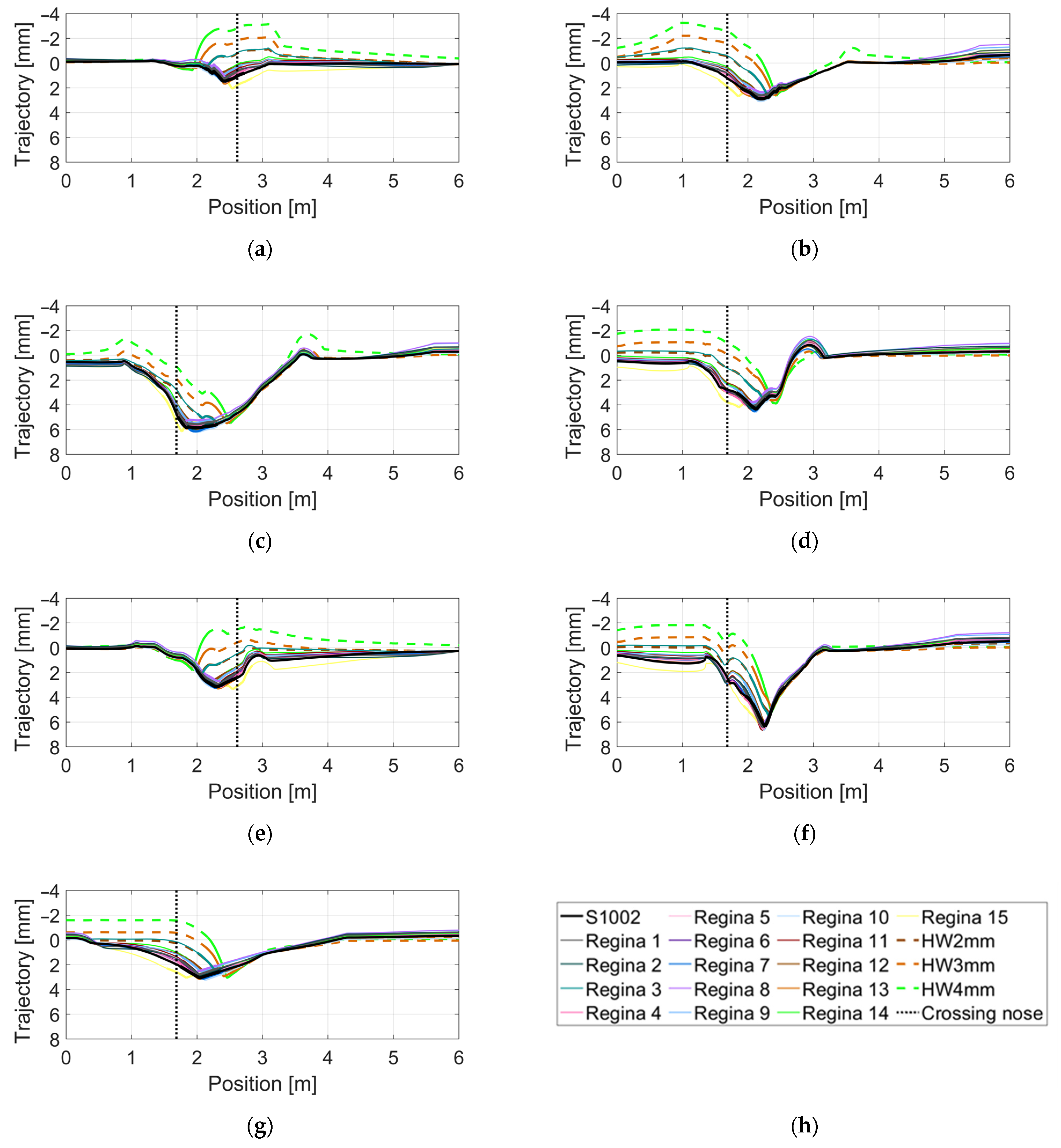
3.2. Wheel Profile Data
3.3. Simulation Setup
4. Observation of Track Response from Crossing Impact Loading
5. MBS Analysis with Nominal Track Model Parameters: Influence of Crossing Geometry
6. Calibration of MBS Track Model Parameters
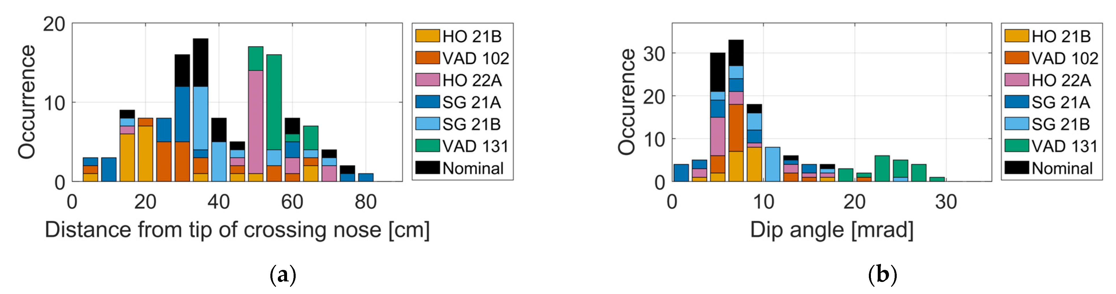
7. Agreement between Measured and Simulated Crossing Condition Indicators
8. Conclusions
8.1. Wheel–Crossing Interaction Kinematics
8.2. Calibration of MBS Models
8.3. Crossing Geometry Condition Indicator
Author Contributions
Funding
Institutional Review Board Statement
Informed Consent Statement
Data Availability Statement
Acknowledgments
Conflicts of Interest
References
- Increased Capacity 4 Rail Networks through Enhanced Infrastructure and Optimized Operations, Deliverable D13.1 Operational Failure Modes of S&C; European Commission: Brussels, Belgium, 2015.
- Skrypnyk, R.; Ossberger, U.; Pålsson, B.A.; Ekh, M.; Nielsen, J.C.O. Long-term rail profile damage in a railway crossing: Field measurements and numerical simulations. Wear 2021, 472, 203331. [Google Scholar] [CrossRef]
- Cornish, A. Life-Time Monitoring of in Service Switches and Crossings through Field Experimentation. Ph.D. Thesis, Imperial College London, London, UK, 2014. [Google Scholar]
- Zhai, W. Vehicle–Track Coupled Dynamics: Theory and Applications; Springer Nature: Basingstoke, UK, 2019. [Google Scholar]
- Liu, X.; Markine, V.L.; Wang, H.; Shevtsov, I.Y. Experimental tools for railway crossing condition monitoring (crossing condition monitoring tools). Measurement 2018, 129, 424–435. [Google Scholar] [CrossRef]
- In2Track, Deliverable 2.2, Enhanced S&C Whole System Analysis, Design and Virtual Validation, Chapter 3, Project Shift 2 Rail. Available online: https://projects.shift2rail.org/download.aspx?id=51f4ad7e-3dc1-418c-8744-97f861c4cf95 (accessed on 20 November 2021).
- Bezin, Y.; Grossoni, I.; Neves, S. Impact of wheel shape on the vertical damage of cast crossing panels in turnouts. In Proceedings of the 24th International Symposium on Dynamics of Vehicles on Roads and Tracks, Graz, Austria, 17–21 August 2015. [Google Scholar]
- Pålsson, B.A. A parameterized turnout model for simulation of dynamic vehicle-turnout interaction with an application to crossing geometry assessment. In Proceedings of the IAVSD International Symposium on Dynamics of Vehicles on Roads and Tracks, Gothenburg, Sweden, 12–16 August 2019; Springer: Berlin/Heidelberg, Germany, 2019; pp. 351–358. [Google Scholar]
- Torstensson, P.; Squicciarini, G.; Krüger, M.; Pålsson, B.A.; Nielsen, J.C.O.; Thompson, D.J. Wheel–rail impact loads and noise generated at railway crossings–Influence of vehicle speed and crossing dip angle. J. Sound Vib. 2019, 456, 119–136. [Google Scholar] [CrossRef]
- Liu, X.; Markine, V.L. Train hunting related fast degradation of a railway crossing—Condition monitoring and numerical verification. Sensors 2020, 20, 2278. [Google Scholar] [CrossRef] [Green Version]
- Bruni, S.; Anastasopoulos, I.; Alfi, S.; Van Leuven, A.; Gazetas, G. Effects of train impacts on urban turnouts: Modelling and validation through measurements. J. Sound Vib. 2009, 324, 666–689. [Google Scholar] [CrossRef]
- Grossoni, I.; Bezin, Y.; Neves, S. Optimisation of support stiffness at railway crossings. Veh. Syst. Dyn. 2018, 56, 1072–1096. [Google Scholar] [CrossRef] [Green Version]
- Pletz, M.; Daves, W.; Ossberger, H. A wheel set/crossing model regarding impact, sliding and deformation—Explicit finite element approach. Wear 2012, 294, 446–456. [Google Scholar] [CrossRef]
- Xin, L.; Markine, V.; Shevtsov, I. Numerical analysis of the dynamic interaction between wheel set and turnout crossing using the explicit finite element method. Veh. Syst. Dyn. 2016, 54, 301–327. [Google Scholar] [CrossRef] [Green Version]
- Boogaard, M.; Li, Z.; Dollevoet, R. In situ measurements of the crossing vibrations of a railway turnout. Measurement 2018, 125, 313–324. [Google Scholar] [CrossRef]
- Milosevic, M.D.G.; Pålsson, B.A.; Nissen, A.; Nielsen, J.C.O.; Johansson, H. Reconstruction of sleeper displacements from measured accelerations for model-based condition monitoring of railway crossing panels. 2021; Submitted for international publication. [Google Scholar]
- Kampczyk, A.; Dybeł, K. The Fundamental Approach of the Digital Twin Application in Railway Turnouts with Innovative Monitoring of Weather Conditions. Sensors 2021, 21, 5757. [Google Scholar] [CrossRef]
- Taştimur, C.; Karaköse, M.; Erhan, A. A vision based condition monitoring approach for rail switch and level crossing using hierarchical SVM in railways. Int. J. Appl. Math. Electron. Comput. 2016, 319–325. [Google Scholar] [CrossRef] [Green Version]
- HandySCAN 3D—Black Series. The Truly Portable Metrology-Grade 3D Scanners. Available online: https://www.creaform3d.com/en/portable-3d-scanner-handyscan-3d (accessed on 20 November 2021).
- Han, D. Comparison of commonly used image interpolation methods. In Proceedings of the 2nd International Conference on Computer Science and Electronics Engineering, Hangzhou, China, 22–23 March 2013; Atlantis Press: Dordrecht, The Netherlands, 2013; pp. 1556–1559. [Google Scholar]
- Next generation KONUX IoT Device. Available online: https://www.konux.com/ (accessed on 20 November 2021).
- Bezin, Y.; Pålsson, B.A. Multibody simulation benchmark for dynamic vehicle-track interaction in switches and crossings: Modelling description and simulation tasks. Veh. Syst. Dyn. 2021, 1–16. [Google Scholar] [CrossRef]
- Kalker, J.J. A fast algorithm for the simplified theory of rolling contact. Veh. Syst. Dyn. 1982, 11, 1–13. [Google Scholar] [CrossRef]
- Sysyn, M.; Nabochenko, O.; Kovalchuk, V. Experimental investigation of the dynamic behavior of railway track with sleeper voids. Railw. Eng. Sci. 2020, 28, 290–304. [Google Scholar] [CrossRef]
- Pålsson, B.A.; Nielsen, J.C.O. Wheel-rail interaction and damage in switches and crossings. Veh. Syst. Dyn. 2012, 50, 43–58. [Google Scholar] [CrossRef]
- Pålsson, B.A.; Nielsen, J.C.O. Track gauge optimisation of railway switches using a genetic algorithm. Veh. Syst. Dyn. 2012, 50, 365–387. [Google Scholar] [CrossRef]
- Pålsson, B.A. A linear wheel–crossing interaction model. Proc. Inst. Mech. Eng. Part F J. Rail Rapic Transit 2018, 232, 2431–2443. [Google Scholar] [CrossRef]
- Iwnicki, S. Manchester benchmarks for rail vehicle simulation. Veh. Syst. Dyn. 1998, 30, 295–313. [Google Scholar] [CrossRef]
- Milne, D.; Masoudi, A.; Ferro, E.; Watson, G.; Le Pen, L. An analysis of railway track behaviour based on distributed optical fibre acoustic sensing. Mech. Syst. Signal Process. 2020, 142, 106769. [Google Scholar] [CrossRef]
- Jenkins, H.; Stephenson, J.; Clayton, G.; Morland, G.; Lyon, D. The effect of track and vehicle parameters on wheel/rail vertical dynamic forces. Railw. Eng. J. 1974, 3, 2–16. [Google Scholar]
- Pålsson, B.A.; Nielsen, J.C.O. Dynamic vehicle-track interaction in switches and crossings and the influence of rail pad stiffness—Field measurements and validation of a simulation model. Veh. Syst. Dyn. 2015, 53, 734–755. [Google Scholar] [CrossRef]
- Nicklisch, D.; Nielsen, J.C.O.; Ekh, M.; Johansson, A.; Pålsson, B.; Zoll, A.; Reinecke, J. Simulation of wheel–rail contact and subsequent material degradation in switches & crossings. In Proceedings of the 21st International Symposium on Dynamics of Vehicles on Roads and Tracks, Stockholm, Sweden, 17–21 August 2009. [Google Scholar]
- Xu, L.; Liu, X. Matrix coupled model for the vehicle–track interaction analysis featured to the railway crossing. Mech. Syst. Signal Process. 2021, 152, 107485. [Google Scholar] [CrossRef]
- Schober, P.; Boer, C.; Schwarte, L.A. Correlation coefficients: Appropriate use and interpretation. Anesth. Analg. 2018, 126, 1763–1768. [Google Scholar] [CrossRef] [PubMed]
- Montgomery, D.C.; Peck, E.A.; Vining, G.G. Introduction to Linear Regression Analysis; John Wiley & Sons: New York, NY, USA, 2021. [Google Scholar]
- Takemiya, H. Simulation of track-ground vibrations due to a high-speed train: The case of X-2000 at Ledsgård. J. Sound Vib. 2003, 261, 503–526. [Google Scholar] [CrossRef]


| Location | Höör | Höör | Stehag | Stehag | Vätteryd | Vätteryd |
|---|---|---|---|---|---|---|
| Crossing name | 21B | 22A | 21A | 21B | 102 | 131 |
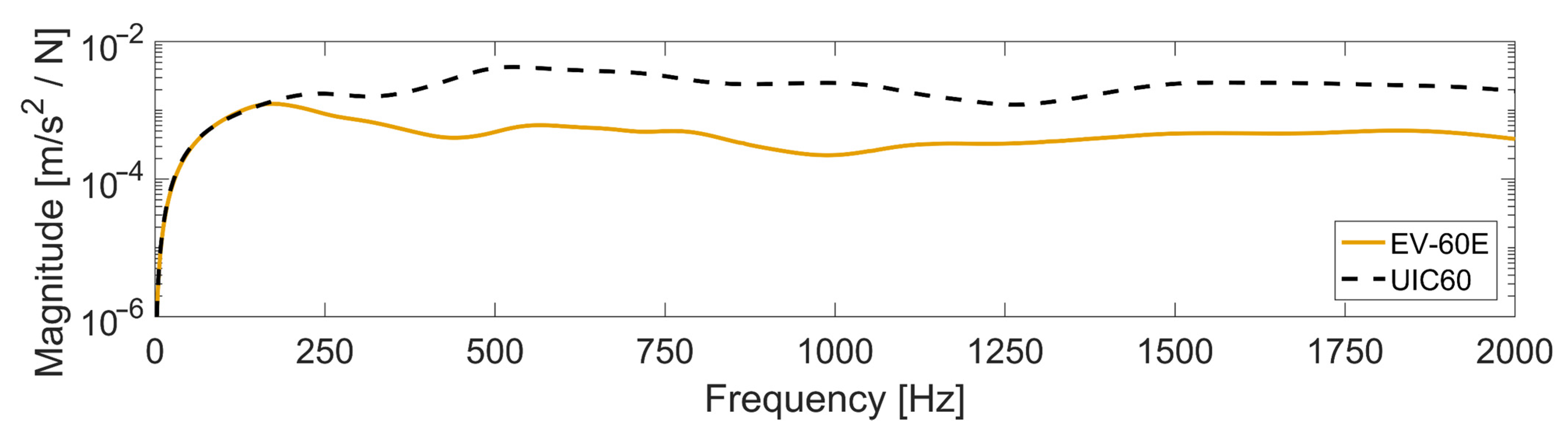
| Design | EV-60E 1:18.5 | EV-60E 1:18.5 | UIC60 1:18.5 | UIC60 1:18.5 | UIC60 1:18.5 | UIC60 1:18.5 |
| Direction | Trailing | Facing | Facing | Facing | Trailing | Facing |
| Radius | 1200 m | 1200 m | 1200 m | 1200 m | 1200 m | 1200 m |
| Crossing rail installation date | 2014 | 2014 | 2018 | 2012 | 2014 | 2014 |
| Scanning date | 4 June 2019 | |||||
| Scanner Information | |
|---|---|
| Device | PorTable 3D laser scanner |
| Accuracy | 0.035 mm |
| Volumetric accuracy | 0.02 mm + 0.06 mm/m |
| Measurement resolution | 0.025 mm |
| Mesh resolution | 0.1 mm |
| Measurement rate | 800,000 measurements/s |
| Light source | 7 laser crosses |
| Scanning area | 310 × 350 mm |
| Device | Monoaxial Cellular Accelerometer |
|---|---|
| Installation | Permanent sleeper connection |
| Direction of measurements | Vertical |
| Sampling rate | 2 kHz |
| Range | ±50 g or ±100 g Depending on crossing panel |
| MBS Model Components | Value | |
|---|---|---|
| Vehicle | Type | Single bogie [28] |
| Wheel radius [m] | 0.46 | |
| Wheelset mass [kg] | 1340 | |
| Axle load [kg] | 15,500 | |
| Axle spacing [m] | 2.9 | |
| Rail * | Element type | Timoshenko beam |
| Lengthwise node spacing [m] | 0.3 | |
| Profile | 60E1 | |
| Young’s modulus [GPa] | 210 | |
| Mass density [kg/meter rail] | 60 | |
| Rail pads | Element type | Kelvin bushing elements |
| Vertical stiffness [MN/m] | 1200 (UIC60) 60 (EV-60E) | |
| Vertical damping [kNs/m] | 25 (UIC60) 6 (EV-60E) | |
| Sleeper | Element type | Timoshenko beam |
| Lengthwise node spacing [m] | 0.25 average | |
| Young’s modulus [GPa] | 30 | |
| Mass density [kg/m3] | 2400 | |
| Ballast | Element type | Kelvin bushing elements |
| Vertical stiffness [MN/m/m] | 30 | |
| Vertical damping [kNs/m/m] | 125 | |
| Feature Name | Case 1—Nominal | Case 2—Soft Pad | Case 3—Calibration |
|---|---|---|---|
| Wheel profiles | 19 | 19 | 19 |
| Crossing panels | 6 scanned + 1 nominal (7) | 6 scanned + 1 nominal (7) | 6 scanned |
| Train speed [km/h] | 160 | 160 | various |
| Total number of simulations | 133 | 133 | 114 |
| Calibration Parameters | |||||||||
|---|---|---|---|---|---|---|---|---|---|
| Crossing Panel | Ballast Vertical Stiffness [MN/m/m] | Ballast Vertical Damping [kNs/m/m] | Rail Pad Vertical Stiffness [MN/m] | Rail Pad Vertical Damping [kNs/m] | Number of Voided Sleepers | Sleeper Void [mm] | Crossing and Stock Rail Flexural Stiffness | RMS Error Measurem-ents and Simulations | Train Speed [km/h] |
| HO 21B | 15 | 75 | 50 | 12 | 0 | 0 | 100% | 0.037 | 160 |
| HO 22A | 20 | 60 | 60 | 12 | 2 | 0.55 | 100% | 0.052 | 190 |
| SG 21A | 20 | 50 | 1200 | 120 | 3 | 1.00 | 100% | 0.085 | 160 |
| SG 21B | 20 | 50 | 1200 | 120 | 3 | 2.00 | 100% | 0.149 | 160 |
| VAD 102 | 12 | 50 | 1200 | 120 | 0 | 0 | 100% | 0.138 | 190 |
| VAD 131 | 10 | 50 | 1200 | 120 | 4 | 5.00 | 75–85% | 0.358 | 130 |
Publisher’s Note: MDPI stays neutral with regard to jurisdictional claims in published maps and institutional affiliations. |
© 2022 by the authors. Licensee MDPI, Basel, Switzerland. This article is an open access article distributed under the terms and conditions of the Creative Commons Attribution (CC BY) license (https://creativecommons.org/licenses/by/4.0/).
Share and Cite
Milosevic, M.D.G.; Pålsson, B.A.; Nissen, A.; Nielsen, J.C.O.; Johansson, H. Condition Monitoring of Railway Crossing Geometry via Measured and Simulated Track Responses. Sensors 2022, 22, 1012. https://doi.org/10.3390/s22031012
Milosevic MDG, Pålsson BA, Nissen A, Nielsen JCO, Johansson H. Condition Monitoring of Railway Crossing Geometry via Measured and Simulated Track Responses. Sensors. 2022; 22(3):1012. https://doi.org/10.3390/s22031012
Chicago/Turabian StyleMilosevic, Marko D. G., Björn A. Pålsson, Arne Nissen, Jens C. O. Nielsen, and Håkan Johansson. 2022. "Condition Monitoring of Railway Crossing Geometry via Measured and Simulated Track Responses" Sensors 22, no. 3: 1012. https://doi.org/10.3390/s22031012