
Experimental Shape Sensing and Load Identification on a Stiffened Panel: A Comparative Study


Abstract
:1. Introduction
2. Methods
2.1. The Modal Method
2.2. The Inverse Finite Element Method
2.3. The 2-Step Method
3. Experimental Setup and Preliminary Computations
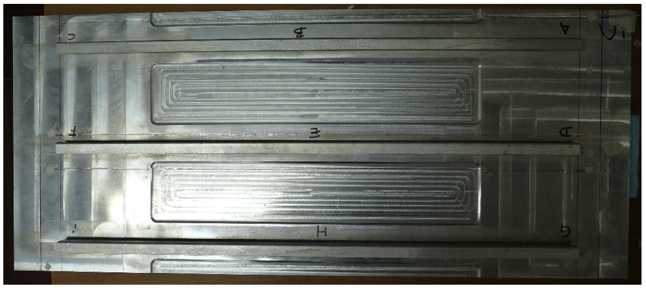
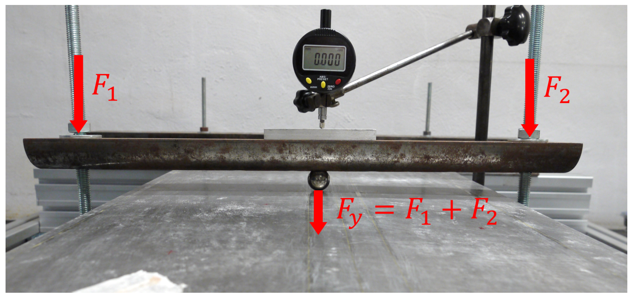
3.1. Experimental Setup
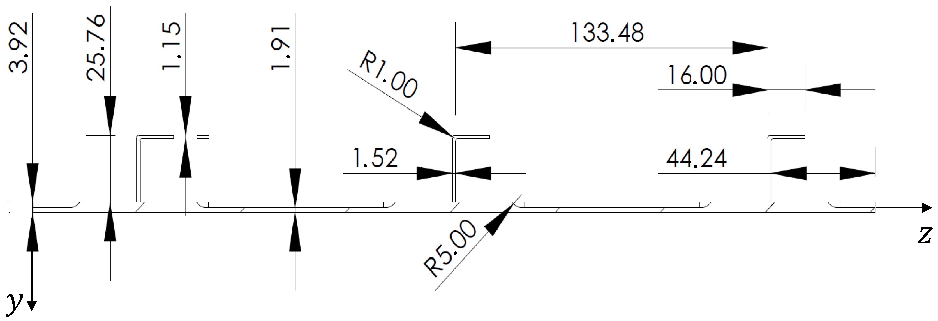
3.2. Models
3.3. Configuration of Sensors
4. Experimental Results
5. Conclusions
Author Contributions
Funding
Institutional Review Board Statement
Informed Consent Statement
Data Availability Statement
Acknowledgments
Conflicts of Interest
Appendix A. Experimental Strains


References
- Colombo, L.; Sbarufatti, C.; Giglio, M. Definition of a load adaptive baseline by inverse finite element method for structural damage identification. Mech. Syst. Signal Process. 2019, 120, 584–607. [Google Scholar] [CrossRef]
- Roy, R.; Gherlone, M.; Surace, C.; Tessler, A. Full-Field strain reconstruction using uniaxial strain measurements: Application to damage detection. Appl. Sci. 2021, 11, 1681. [Google Scholar] [CrossRef]
- Li, M.; Kefal, A.; Cerik, B.C.; Oterkus, E. Dent damage identification in stiffened cylindrical structures using inverse Finite Element Method. Ocean. Eng. 2020, 198, 106944. [Google Scholar] [CrossRef]
- Colombo, L.; Oboe, D.; Sbarufatti, C.; Cadini, F.; Russo, S.; Giglio, M. Shape sensing and damage identification with iFEM on a composite structure subjected to impact damage and non-trivial boundary conditions. Mech. Syst. Signal Process. 2021, 148, 107163. [Google Scholar] [CrossRef]
- Airoldi, A.; Sala, G.; Evenblij, R.; Koimtzoglou, C.; Loutas, T.; Carossa, G.M.; Mastromauro, P.; Kanakis, T. Load monitoring by means of optical fibres and strain gages. In Smart Intelligent Aircraft Structures (SARISTU); Wölcken, P.C., Papadopoulos, M., Eds.; Springer International Publishing: Cham, Switzerland, 2016; pp. 433–469. [Google Scholar] [CrossRef]
- Nakamura, T.; Igawa, H.; Kanda, A. Inverse identification of continuously distributed loads using strain data. Aerosp. Sci. Technol. 2012, 23, 75–84. [Google Scholar] [CrossRef]
- Barbarino, S.; Bilgen, O.; Ajaj, R.M.; Friswell, M.I.; Inman, D.J. A review of morphing aircraft. J. Intell. Mater. Syst. Struct. 2011, 22, 823–877. [Google Scholar] [CrossRef]
- de Souza Siqueira Versiani, T.; Silvestre, F.J.; Guimarães Neto, A.B.; Rade, D.A.; Annes da Silva, R.G.; Donadon, M.V.; Bertolin, R.M.; Silva, G.C. Gust load alleviation in a flexible smart idealized wing. Aerosp. Sci. Technol. 2019, 86, 762–774. [Google Scholar] [CrossRef]
- Soller, B.J.; Gifford, D.K.; Wolfe, M.S.; Froggatt, M.E. High resolution optical frequency domain reflectometry for characterization of components and assemblies. Opt. Express 2005, 13, 666–674. [Google Scholar] [CrossRef] [Green Version]
- Di Sante, R. Fibre optic sensors for structural health monitoring of aircraft composite structures: Recent advances and applications. Sensors 2015, 15, 18666–18713. [Google Scholar] [CrossRef]
- Ko, W.L.; Richards, W.L.; Fleischer, V.T. Displacement Theories for In-Flight Deformed Shape Predictions of Aerospace Structures; Report NASA/TP-2007-214612; NASA Dryden Flight Research Center: Edwards, CA, USA, 2007. [Google Scholar]
- Pak, C. Wing Shape Sensing from Measured Strain. AIAA J. 2016, 54, 1068–1077. [Google Scholar] [CrossRef] [Green Version]
- Ding, G.; Yue, S.; Zhang, S.; Song, W. Strain—Deformation reconstruction of CFRP laminates based on Ko displacement theory. Nondestruct. Test. Eval. 2020, 36, 1–13. [Google Scholar] [CrossRef]
- Foss, G.; Haugse, E. Using modal test results to develop strain to displacement transformations. In Proceedings of the 13th International Modal Analysis Conference, Nashville, TN, USA, 13–16 February 1995. [Google Scholar]
- Bogert, P.; Haugse, E.; Gehrki, R. Structural shape identification from experimental strains using a modal transformation technique. In Proceedings of the 44th AIAA/ASME/ASCE/AHS/ASC Structures, Structural Dynamics, and Materials Conference, Norfolk, VA, USA, 7–10 April 2012. [Google Scholar] [CrossRef]
- Freydin, M.; Rattner, M.K.; Raveh, D.E.; Kressel, I.; Davidi, R.; Tur, M. Fiber-optics-based aeroelastic shape sensing. AIAA J. 2019, 57, 5094–5103. [Google Scholar] [CrossRef]
- Bruno, R.; Toomarian, N.; Salama, M. Shape estimation from incomplete measurements: A neural-net approach. Smart Mater. Struct. 1994, 3, 92–97. [Google Scholar] [CrossRef]
- Mao, Z.; Todd, M. Comparison of shape reconstruction strategies in a complex flexible structure. In Sensors and Smart Structures Technologies for Civil, Mechanical, and Aerospace Systems 2008; Tomizuka, M., Ed.; International Society for Optics and Photonics: Bellingham, WA, USA, 2008; Volume 6932, pp. 127–138. [Google Scholar]
- Gherlone, M.; Cerracchio, P.; Mattone, M. Shape sensing methods: Review and experimental comparison on a wing-shaped plate. Prog. Aerosp. Sci. 2018, 99, 14–26. [Google Scholar] [CrossRef]
- Esposito, M.; Gherlone, M. Composite wing box deformed-shape reconstruction based on measured strains: Optimization and comparison of existing approaches. Aerosp. Sci. Technol. 2020, 99, 105758. [Google Scholar] [CrossRef]
- Esposito, M.; Gherlone, M. Material and strain sensing uncertainties quantification for the shape sensing of a composite wing box. Mech. Syst. Signal Process. 2021, 160, 107875. [Google Scholar] [CrossRef]
- Pisoni, A.C.; Santolini, C.; Hauf, D.E.; Dubowsky, S. Displacements in a vibrating body by strain gauge measurements. In Proceedings of the 13th International Modal Analysis Conference, Nashville, TN, USA, 13–16 February 1995. [Google Scholar]
- Tessler, A.; Spangler, J.L. A Variational Principle for Reconstruction of Elastic Deformations in Shear Deformable Plates and Shells; Report NASA/TM-2003-212445; NASA Langley Research Center: Hampton, VA, USA, 2003. [Google Scholar]
- Gherlone, M.; Cerracchio, P.; Mattone, M.; Sciuva, M.D.; Tessler, A. Shape sensing of 3D frame structures using an inverse Finite Element Method. Int. J. Solids Struct. 2012, 49, 3100–3112. [Google Scholar] [CrossRef] [Green Version]
- Gherlone, M.; Cerracchio, P.; Mattone, M.; Sciuva, M.D.; Tessler, A. An inverse finite element method for beam shape sensing: Theoretical framework and experimental validation. Smart Mater. Struct. 2014, 23, 045027. [Google Scholar] [CrossRef] [Green Version]
- Zhao, F.; Xu, L.; Bao, H.; Du, J. Shape sensing of variable cross-section beam using the inverse finite element method and isogeometric analysis. Measurement 2020, 158, 107656. [Google Scholar] [CrossRef]
- Roy, R.; Gherlone, M.; Surace, C. A shape sensing methodology for beams with generic cross-sections: Application to airfoil beams. Aerosp. Sci. Technol. 2021, 110, 106484. [Google Scholar] [CrossRef]
- Papa, U.; Russo, S.; Lamboglia, A.; Core, G.D.; Iannuzzo, G. Health structure monitoring for the design of an innovative UAS fixed wing through inverse finite element method (iFEM). Aerosp. Sci. Technol. 2017, 69, 439–448. [Google Scholar] [CrossRef]
- Tessler, A.; Spangler, J.L. Inverse FEM for full-field reconstruction of elastic deformations in shear deformable plates and shells. In Proceedings of the 2nd European Workshop on Structural Health Monitoring, Munich, Germany, 7–9 July 2004. [Google Scholar]
- Cerracchio, P.; Gherlone, M.; Tessler, A. Real-time displacement monitoring of a composite stiffened panel subjected to mechanical and thermal loads. Meccanica 2015, 50, 2487–2496. [Google Scholar] [CrossRef]
- Miller, E.J.; Manalo, R.; Tessler, A. Full-Field Reconstruction of Structural Defor- mations and Loads from Measured Strain Data on a Wing Using the Inverse Finite Element Method; Report NASA/TM-2016-219407; NASA Dryden Flight Research Center: Edwards, CA, USA, 2016. [Google Scholar]
- Kefal, A.; Tabrizi, I.E.; Yildiz, M.; Tessler, A. A smoothed iFEM approach for efficient shape-sensing applications: Numerical and experimental validation on composite structures. Mech. Syst. Signal Process. 2021, 152, 107486. [Google Scholar] [CrossRef]
- Kefal, A.; Oterkus, E. Displacement and stress monitoring of a chemical tanker based on inverse finite element method. Ocean Eng. 2016, 112, 33–46. [Google Scholar] [CrossRef] [Green Version]
- Kefal, A.; Oterkus, E. Displacement and stress monitoring of a Panamax containership using inverse finite element method. Ocean Eng. 2016, 119, 16–29. [Google Scholar] [CrossRef] [Green Version]
- Kefal, A.; Oterkus, E.; Tessler, A.; Spangler, J.L. A quadrilateral inverse-shell element with drilling degrees of freedom for shape sensing and structural health monitoring. Eng. Sci. Technol. Int. J. 2016, 19, 1299–1313. [Google Scholar] [CrossRef] [Green Version]
- Kefal, A.; Oterkus, E. Isogeometric iFEM analysis of thin shell structures. Sensors 2020, 20, 2685. [Google Scholar] [CrossRef]
- Oboe, D.; Colombo, L.; Sbarufatti, C.; Giglio, M. Shape sensing of a complex aeronautical structure with inverse Finite Element Method. Sensors 2021, 21, 1388. [Google Scholar] [CrossRef]
- Shkarayev, S.; Krashanitsa, R.; Tessler, A. An inverse interpolation method utilizing in-flight strain measurements for determining loads and structural response of aerospace vehicles. In Proceedings of the 3rd Intrnational Workshop on Structural Health Monitoring, Stanford, CA, USA, 12–14 September 2001. [Google Scholar]
- Coates, C.; Thamburaj, P.; Kim, C. An inverse method for selection of Fourier coefficients for flight load identification. In Proceedings of the 46th AIAA/ASME/ ASCE/AHS/ASC Structures, Structural Dynamics and Materials Conference, Austin, TX, USA, 18–25 April 2005. [Google Scholar] [CrossRef]
- Coates, C.W.; Thamburaj, P. Inverse method using finite strain measurements to determine flight load distribution functions. J. Aircr. 2008, 45, 366–370. [Google Scholar] [CrossRef]
- Liu, H.; Liu, Q.; Liu, B.; Tang, X.; Ma, H.; Pan, Y.; Fish, J. An efficient and robust method for structural distributed load identification based on mesh superposition approach. Mech. Syst. Signal Process. 2021, 151, 107383. [Google Scholar] [CrossRef]
- Airoldi, A.; Marelli, L.; Bettini, P.; Sala, G.; Apicella, A. Strain field reconstruction on composite spars based on the identification of equivalent load conditions. In Sensors and Smart Structures Technologies for Civil, Mechanical, and Aerospace Systems 2017; Lynch, J.P., Ed.; International Society for Optics and Photonics: Bellingham, WA, USA, 2017; Volume 10168, pp. 207–226. [Google Scholar] [CrossRef]
- Esposito, M.; Gherlone, M.; Marzocca, P. External loads identification and shape sensing on an aluminum wing box: An integrated approach. Aerosp. Sci. Technol. 2021, 114, 106743. [Google Scholar] [CrossRef]
- Penrose, R. On best approximate solutions of linear matrix equations. Math. Proc. Camb. Philos. Soc. 1956, 52, 17–19. [Google Scholar] [CrossRef]
- Mindlin, R. Influence of rotatory inertia and shear deformation on flexural motions of isotropic elastic plates. J. Appl. Mech. 1951, 18, 31–138. [Google Scholar] [CrossRef]


| Al-Li Alloy | |
|---|---|
| 75,958 | |
| 0.300 | |
| 2.78 |
| Experimental | HF-FEM | 2-Step | MM (1–22) | MM | iFEM | |
|---|---|---|---|---|---|---|
| Test 1 | ||||||
| −865.0 | −883.1 | |||||
| () | (+2.1%) | |||||
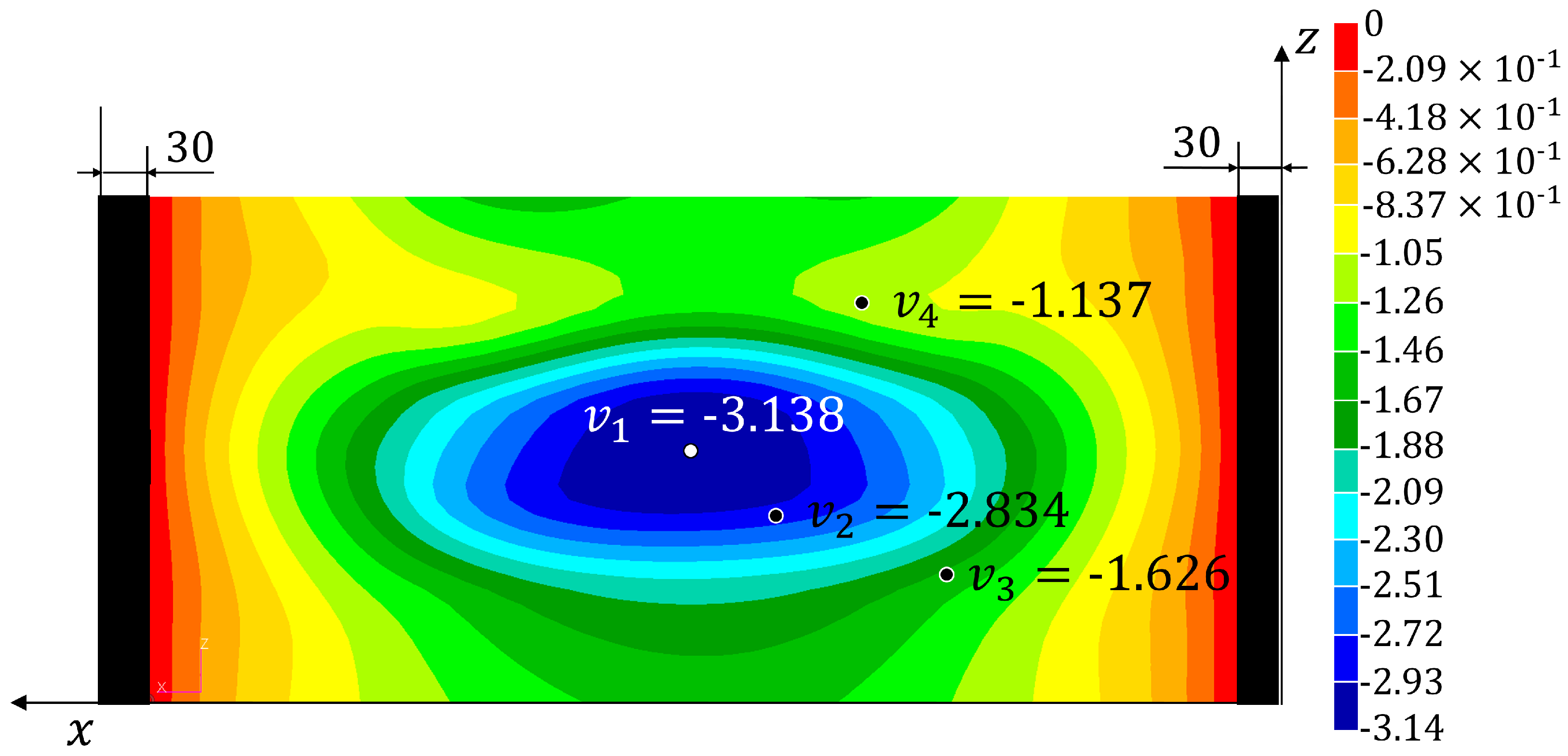
| −3.000 | −3.078 | −3.142 | −3.081 | −3.047 | −2.916 | |
| () | (+2.6%) | (+4.7%) | (+2.7%) | (+1.6%) | (−2.8%) | |
| −2.644 | −2.752 | −2.809 | −2.823 | −2.705 | −2.624 | |
| () | (+4.1%) | (+6.2%) | (+6.8%) | (+2.3%) | (−0.8%) | |
| −1.614 | −1.660 | −1.695 | −1.653 | −1.627 | −1.641 | |
| () | (+2.9%) | (+5.0%) | (+2.4%) | (+0.8%) | (+1.7%) | |
| −1.610 | −1.600 | −1.633 | −1.058 | −1.475 | −1.562 | |
| () | (−0.6%) | (+1.4%) | (−34.3%) | (−8.4%) | (−3.0%) | |
| Test 2 | ||||||
| −882.0 | −899.9 | |||||
| () | (+2.0%) | |||||
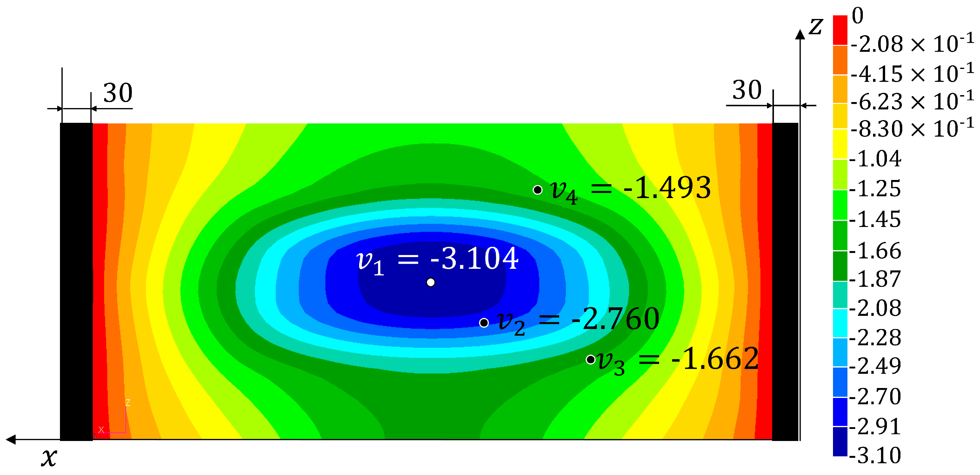
| −3.002 | −3.138 | −3.202 | −3.139 | −3.104 | −2.973 | |
| () | (+4.5%) | (+6.7%) | (+4.6%) | (+3.4%) | (−1.0%) | |
| −2.634 | −2.806 | −2.863 | −2.825 | −2.761 | −2.657 | |
| () | (+6.5%) | (+8.7%) | (+7.3%) | (+4.8%) | (+0.9%) | |
| −1.603 | −1.693 | −1.727 | −1.605 | −1.662 | −1.631 | |
| () | (+5.6%) | (+7.7%) | (+0.1%) | (+3.7%) | (+1.7%) | |
| −1.613 | −1.631 | −1.644 | −1.130 | −1.481 | −1.638 | |
| () | (+1.1%) | (+1.9%) | (−29.9%) | (−8.2%) | (+1.5%) | |
| Test 3 | ||||||
| −882.0 | −899.7 | |||||
| () | (+2.0%) | |||||
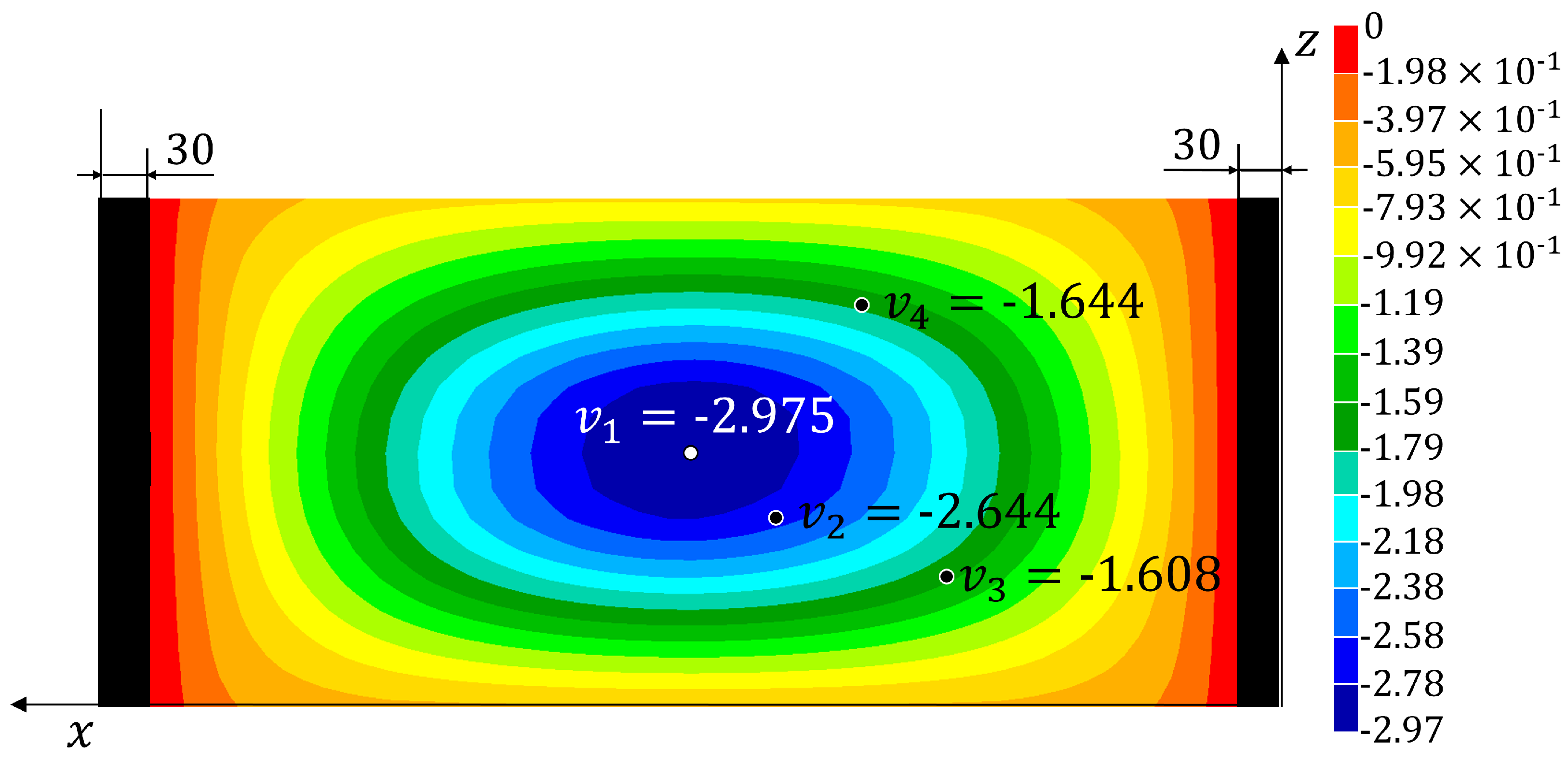
| −3.004 | −3.138 | −3.201 | −3.138 | −3.104 | −2.975 | |
| () | (+4.5%) | (+6.6%) | (+4.5%) | (+3.3%) | (−1.0%) | |
| −2.649 | −2.806 | −2.862 | −2.834 | −2.760 | −2.644 | |
| () | (+5.9%) | (+8.0%) | (+7.0%) | (+4.2%) | (−0.2%) | |
| −1.622 | −1.693 | −1.727 | −1.626 | −1.662 | −1.608 | |
| () | (+4.4%) | (+6.5%) | (+0.2%) | (+2.5%) | (−0.9%) | |
| −1.609 | −1.631 | −1.664 | −1.137 | −1.493 | −1.644 | |
| () | (+1.4%) | (+3.4%) | (−29.3%) | (−7.2%) | (+2.2%) | |
| 2-Step | MM (1–22) | MM | iFEM | |
|---|---|---|---|---|
| 2.0% | ||||
| 6.0% | 3.9% | 2.8% | 1.6% | |
| 7.7% | 7.0% | 3.8% | 0.6% | |
| 6.4% | 0.9% | 2.3% | 1.4% | |
| 2.3% | 31.2% | 7.9% | 2.2% | |
| 5.6% | 10.8% | 4.2% | 1.5% |
Publisher’s Note: MDPI stays neutral with regard to jurisdictional claims in published maps and institutional affiliations. |
© 2022 by the authors. Licensee MDPI, Basel, Switzerland. This article is an open access article distributed under the terms and conditions of the Creative Commons Attribution (CC BY) license (https://creativecommons.org/licenses/by/4.0/).
Share and Cite
Esposito, M.; Mattone, M.; Gherlone, M. Experimental Shape Sensing and Load Identification on a Stiffened Panel: A Comparative Study. Sensors 2022, 22, 1064. https://doi.org/10.3390/s22031064
Esposito M, Mattone M, Gherlone M. Experimental Shape Sensing and Load Identification on a Stiffened Panel: A Comparative Study. Sensors. 2022; 22(3):1064. https://doi.org/10.3390/s22031064
Chicago/Turabian StyleEsposito, Marco, Massimiliano Mattone, and Marco Gherlone. 2022. "Experimental Shape Sensing and Load Identification on a Stiffened Panel: A Comparative Study" Sensors 22, no. 3: 1064. https://doi.org/10.3390/s22031064