
First Gradually, Then Suddenly: Understanding the Impact of Image Compression on Object Detection Using Deep Learning


Abstract
:1. Introduction
- They offer a high object-detection performance that outperforms classical approaches [4];
- They can be trained to detect new classes of objects without programming new algorithms or feature extractors in a human-dependent manual way [5]; and
- Hardware acceleration to address their substantial computational needs is readily available, thus allowing end-to-end training of large models.
1.1. Related Work
1.2. Contribution
- We devise a fully reproducible computational study to thoroughly assess the influence of varying compression levels on the performance of a representative collection of models for object detection (including one-stage and two-stage detection pipelines), using a well-known validation dataset [18].
- We analyze the changes in performance using both an aggregated performance score, as well as separate metrics of recall and precision to allows us to observe differences in behaviors between models in detail.
- We show how different architectures behave with respect to the confidence threshold, and we present the examples of high and low sensitivity to such threshold, which needs to be taken into account while balancing precision and recall.
- We examine the influence of object size (quantified as the object’s area in pixels) on the robustness of object detection.
1.3. Paper Structure
2. Materials and Methods
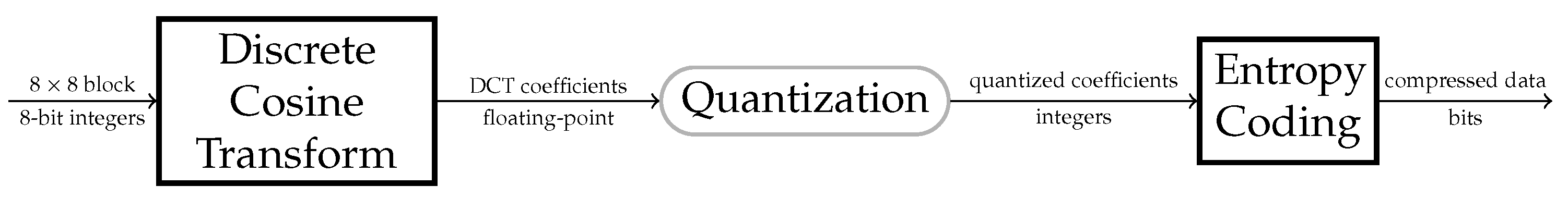
2.1. JPEG Image Compression
2.1.1. Block Transform
2.1.2. Quantization
2.1.3. Setting the JPEG Quality
2.1.4. Relation between the Q Parameter and the Image Quality
2.2. Deep Learning in Object Detection
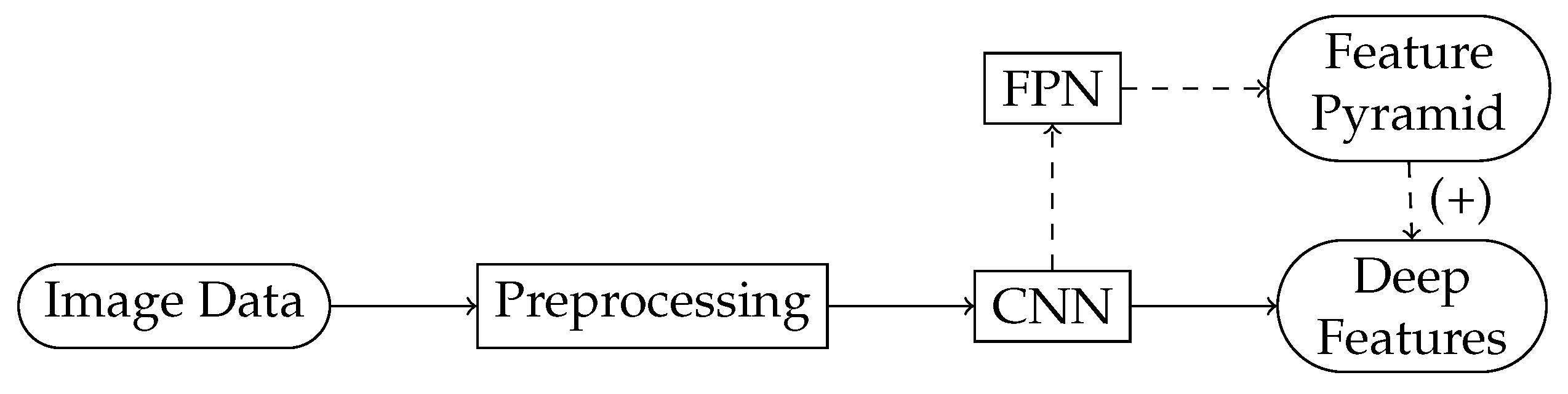
2.2.1. The Object Detection Pipeline
- One- and two-stage detectors (also referred to as the dense and sparse detectors), and
- Detectors, those that use a feature pyramid built on top of the backbone and those that exploit the final convolutional layer of the backbone.
2.2.2. The Backbone for Feature Extraction
2.2.3. Single-Stage Detectors
2.2.4. Two-Stage Detectors
- The region of interest (ROI) proposal mechanism, which generates the locations (boxes) in the image (where an any-class object can be found); when implemented as a neural network, it is known as the region proposal network (RPN).
- The ROI heads, which evaluate the proposals, producing detections.
2.3. Performance Metrics for Object Detection
2.3.1. Assessing a Single Detection
2.3.2. Detecting the Unlabeled Objects: Crowds
2.3.3. Precision, Recall and the F1-Score
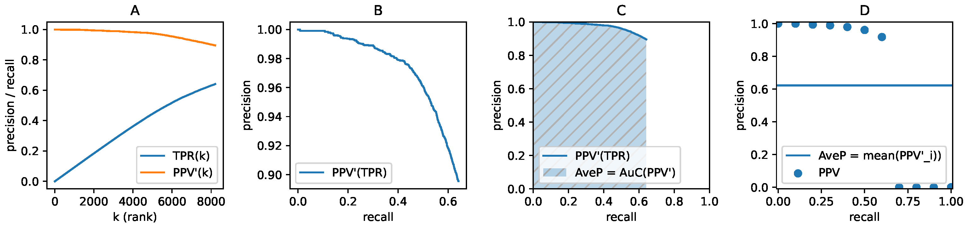
2.3.4. The Precision–Recall Curve and Average Precision
2.3.5. The Performance Metrics Selected for This Study
- TP: the number of true positive detections,
- FP: the number of false positive detections,
- EX: the number of the “extra” (crowd) detections,
- PPV: the overall precision of the detections,
- TPR: the overall recall of the detections,
- F1: the overall F1-score,
- AP: the overall AP metric,
- APs, APm, APl: AP separately for small (below pixels of area), medium (between 1024 and pixels) and large (above 9216 pixels) objects,
- mAP.5, mAP.75: the mean average precision for two different values.
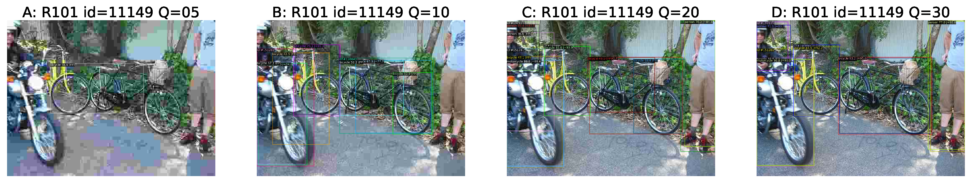
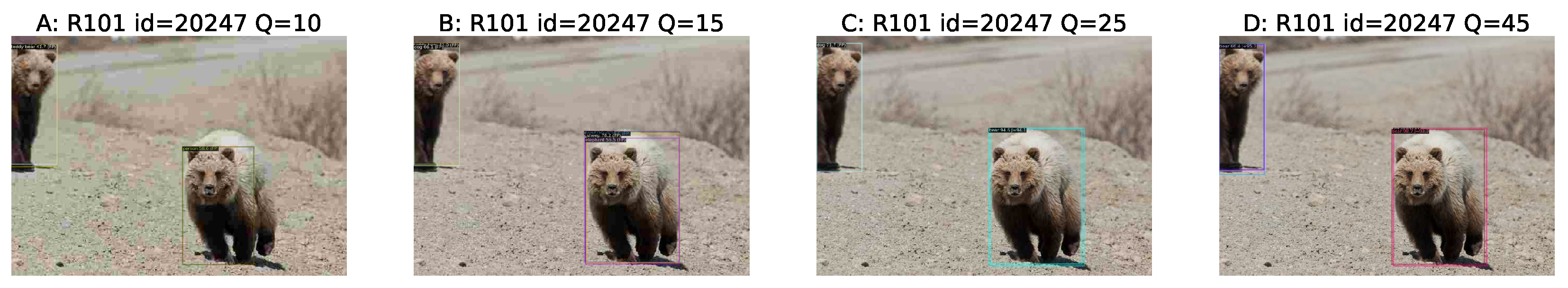
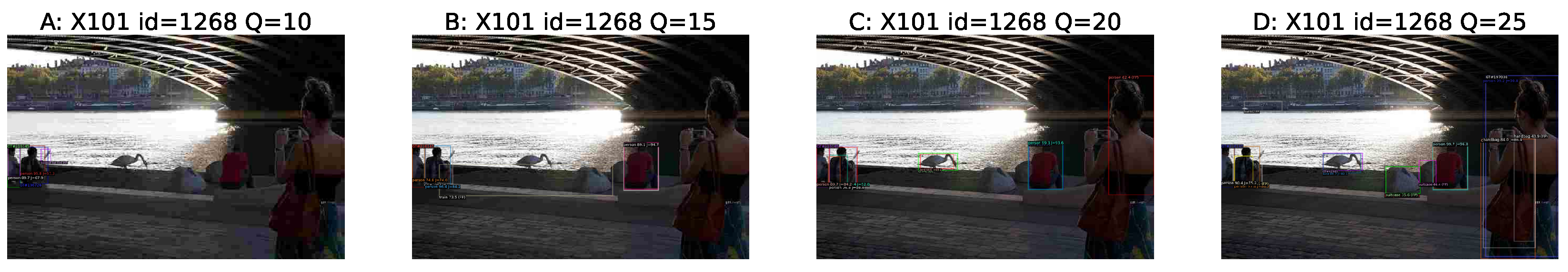
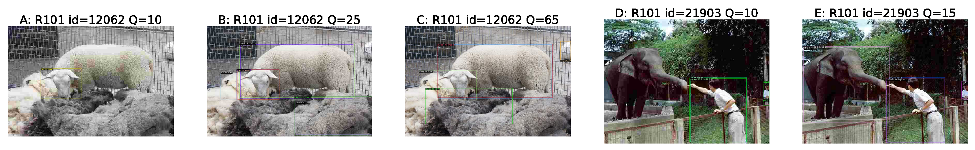
2.4. Qualitative Assessment of the Detection Performance
- omission of an object (FN), the most common error,
- wrong classifications (a bounding box around an object with the wrong category returned, sometimes alongside a correct detection of that very object),
- mistaken objects (detecting real objects with a correct bounding box, but of a category not present in the GT),
- detections of unrelated objects at random places in the image (“halucinating”).
- loss of bounding box accuracy,
- selecting only part of an object or having multiple selections of the object (loss of continuity),
- one box covering multiple objects (cluster) or parts of different objects from the same category (chimera).
2.5. Reproducibility Information
2.5.1. Benchmark Dataset
2.5.2. The Investigated Deep Models
2.5.3. Image Degradation
3. Experimental Results
3.1. The Baseline Results
3.1.1. The AP and Related Metrics
- For AP, the ResNet-101 Faster R-CNNs were only from each other, with the following order of its variants: C4, FPN, DC5.
- For mAP.5, the order was DC5, C4 (), FPN ().
- For mAP.75, the order was FPN, DC5 (), C4 ().
3.1.2. Counting the Objects (TP, FP, EX), Recall and Precision
3.1.3. Discussing the Impact of
3.2. Detection Results on Degraded Images
3.3. Performance Metrics as a Function of Q
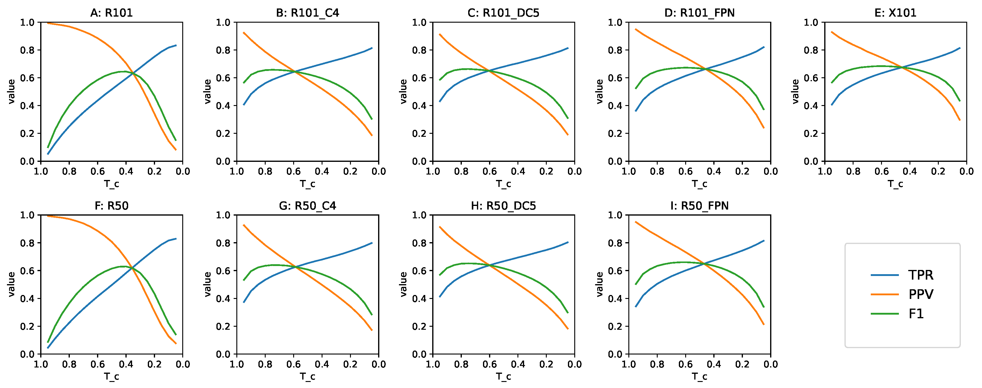
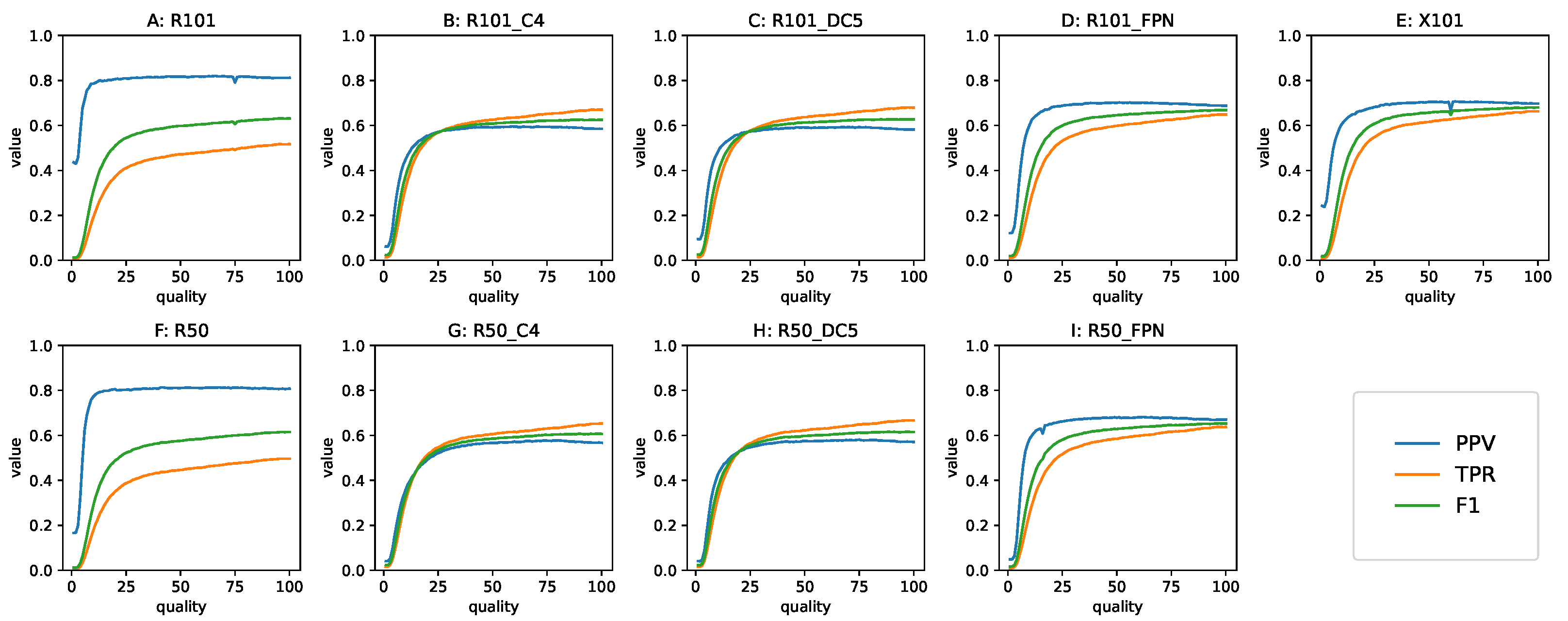
3.3.1. The Precision, Recall and F1 Metrics
3.3.2. The AP, mAP.5 and mAP.75 Metrics
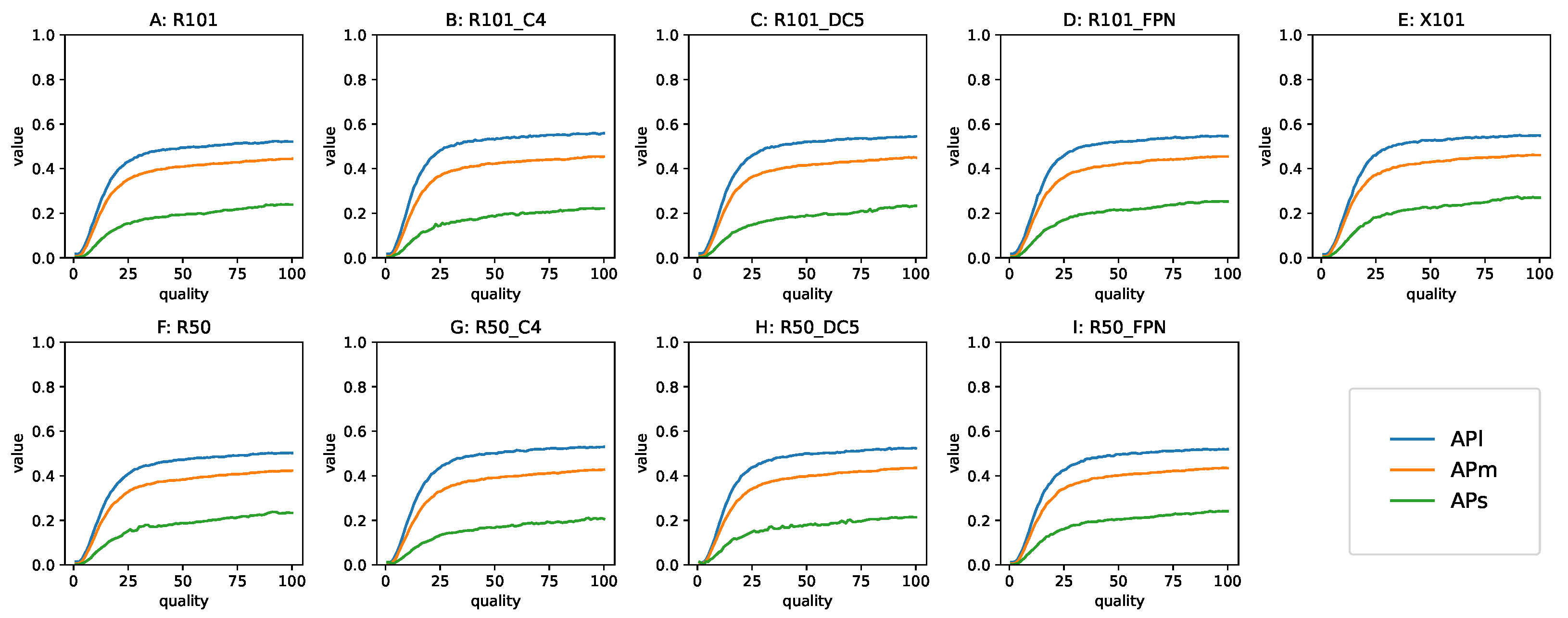
3.3.3. The AP Behavior for Different Sizes of Objects
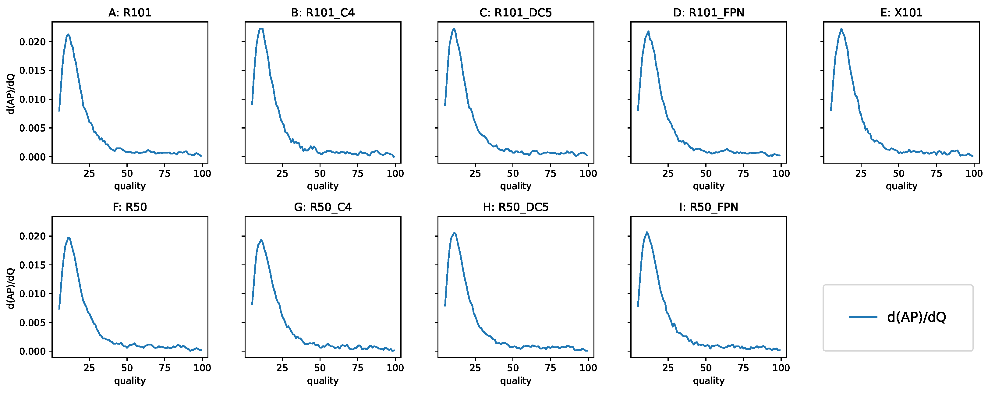
3.3.4. Analyzing the Derivative of AP with Respect to Q
3.3.5. The Metric Values for Stronger Compression
4. Conclusions and Future Work
- Inclusion of more deep-learning-powered object detection models;
- Consideration of related computer vision tasks such as instance segmentation;
Author Contributions
Funding
Institutional Review Board Statement
Informed Consent Statement
Data Availability Statement
Acknowledgments
Conflicts of Interest
Abbreviations
| CNN | convolutional neural network |
| DCT | discrete cosine transform |
| FDCT | forward DCT |
| FN | false negative |
| FP | false positive |
| GT | ground truth |
| IDCT | inverse DCT |
| IoU | intersection over union |
| QT | quantization table |
| ROI | region of interest |
| RPN | region proposal network |
| TP | true positive |
References
- Zelener, A. Object Localization, Segmentation, and Classification in 3D Images. Ph.D. Thesis, The City University of New York, New York, NY, USA, 2018. [Google Scholar]
- Chen, X.; Kundu, K.; Zhang, Z.; Ma, H.; Fidler, S.; Urtasun, R. Monocular 3d object detection for autonomous driving. In Proceedings of the IEEE Conference on Computer Vision and Pattern Recognition, Las Vegas, NV, USA, 27–30 June 2016; pp. 2147–2156. [Google Scholar]
- Dewi, C.; Chen, R.C.; Yu, H.; Jiang, X. Robust detection method for improving small traffic sign recognition based on spatial pyramid pooling. J. Ambient. Intell. Humaniz. Comput. 2021, 1–18. [Google Scholar] [CrossRef]
- Sharma, V.; Mir, R.N. A comprehensive and systematic look up into deep learning based object detection techniques: A review. Comput. Sci. Rev. 2020, 38, 100301. [Google Scholar] [CrossRef]
- Masita, K.L.; Hasan, A.N.; Shongwe, T. Deep Learning in Object Detection: A Review. In Proceedings of the 2020 International Conference on Artificial Intelligence, Big Data, Computing and Data Communication Systems (icABCD), Durban, South Africa, 6–7 August 2020; pp. 1–11. [Google Scholar] [CrossRef]
- Poyser, M.; Atapour-Abarghouei, A.; Breckon, T.P. On the Impact of Lossy Image and Video Compression on the Performance of Deep Convolutional Neural Network Architectures. In Proceedings of the 2020 25th International Conference on Pattern Recognition (ICPR), Milan, Italy, 10–15 January 2021; pp. 2830–2837. [Google Scholar]
- Yang, E.H.; Amer, H.; Jiang, Y. Compression Helps Deep Learning in Image Classification. Entropy 2021, 23, 881. [Google Scholar] [CrossRef] [PubMed]
- Battiato, S.; Mancuso, M.; Bosco, A.; Guarnera, M. Psychovisual and statistical optimization of quantization tables for DCT compression engines. In Proceedings of the 11th International Conference on Image Analysis and Processing, Palermo, Italy, 26–28 September 2001; pp. 602–606. [Google Scholar]
- Ernawan, F.; Abu, N.A.; Suryana, N. TMT quantization table generation based on psychovisual threshold for image compression. In Proceedings of the 2013 International Conference of Information and Communication Technology (ICoICT), Bandung, Indonesia, 20–22 March 2013; pp. 202–207. [Google Scholar]
- Ernawan, F.; Abu, N.A.; Suryana, N. An adaptive JPEG image compression using psychovisual model. Adv. Sci. Lett. 2014, 20, 26–31. [Google Scholar] [CrossRef]
- Siddiqui, S.A.; Dengel, A.; Ahmed, S. Understanding and Mitigating the Impact of Model Compression for Document Image Classification. In Document Analysis and Recognition—ICDAR 2021; Lladós, J., Lopresti, D., Uchida, S., Eds.; Springer: Cham, Switzerland, 2021; pp. 147–159. [Google Scholar]
- Nalepa, J.; Antoniak, M.; Myller, M.; Ribalta Lorenzo, P.; Marcinkiewicz, M. Towards resource-frugal deep convolutional neural networks for hyperspectral image segmentation. Microprocess. Microsystems 2020, 73, 102994. [Google Scholar] [CrossRef]
- Dodge, S.; Karam, L. Understanding how image quality affects deep neural networks. In Proceedings of the 2016 Eighth International Conference on Quality of Multimedia Experience (QoMEX), Lisbon, Portugal, 6–8 June 2016; pp. 1–6. [Google Scholar] [CrossRef] [Green Version]
- Russakovsky, O.; Deng, J.; Su, H.; Krause, J.; Satheesh, S.; Ma, S.; Huang, Z.; Karpathy, A.; Khosla, A.; Bernstein, M.; et al. ImageNet Large Scale Visual Recognition Challenge. Int. J. Comput. Vis. (IJCV) 2015, 115, 211–252. [Google Scholar] [CrossRef] [Green Version]
- Szegedy, C.; Liu, W.; Jia, Y.; Sermanet, P.; Reed, S.; Anguelov, D.; Erhan, D.; Vanhoucke, V.; Rabinovich, A. Going deeper with convolutions. In Proceedings of the IEEE Conference on Computer Vision and Pattern Recognition, Boston, MA, USA, 7–12 June 2015; pp. 1–9. [Google Scholar]
- Goodfellow, I.J.; Shlens, J.; Szegedy, C. Explaining and harnessing adversarial examples. arXiv 2014, arXiv:1412.6572. [Google Scholar]
- Patel, P.; Wong, J.; Tatikonda, M.; Marczewski, J. JPEG compression algorithm using CUDA. In Course Project for ECE; Department of Computer Engineering, University of Toronto: Toronto, ON, Canada, 2009; Volume 1724. [Google Scholar]
- Lin, T.Y.; Maire, M.; Belongie, S.; Hays, J.; Perona, P.; Ramanan, D.; Dollár, P.; Zitnick, C.L. Microsoft coco: Common objects in context. In European Conference on Computer Vision; Springer: Cham, Switzerland, 2014; pp. 740–755. [Google Scholar]
- Ahmed, N.; Natarajan, T.; Rao, K.R. Discrete cosine transform. IEEE Trans. Comput. 1974, 100, 90–93. [Google Scholar] [CrossRef]
- Wallace, G.K. The JPEG still picture compression standard. IEEE Trans. Consum. Electron. 1992, 38, xviii–xxxiv. [Google Scholar] [CrossRef]
- Wang, Z.; Bovik, A.C.; Sheikh, H.R.; Simoncelli, E.P. Image quality assessment: From error visibility to structural similarity. IEEE Trans. Image Process. 2004, 13, 600–612. [Google Scholar] [CrossRef] [Green Version]
- Wang, Z.; Bovik, A.C. A universal image quality index. IEEE Signal Process. Lett. 2002, 9, 81–84. [Google Scholar] [CrossRef]
- Liu, L.; Ouyang, W.; Wang, X.; Fieguth, P.; Chen, J.; Liu, X.; Pietikäinen, M. Deep Learning for Generic Object Detection: A Survey. Int. J. Comput. Vis. 2020, 128, 261–318. [Google Scholar] [CrossRef] [Green Version]
- Bochkovskiy, A.; Wang, C.Y.; Liao, H.Y.M. YOLOv4: Optimal Speed and Accuracy of Object Detection. arXiv 2020, arXiv:2004.10934. [Google Scholar]
- Chen, R.C.; Dewi, C.; Huang, S.W.; Caraka, R.E. Selecting critical features for data classification based on machine learning methods. J. Big Data 2020, 7, 52. [Google Scholar] [CrossRef]
- Lin, T.Y.; Dollár, P.; Girshick, R.; He, K.; Hariharan, B.; Belongie, S. Feature pyramid networks for object detection. In Proceedings of the IEEE Conference on Computer Vision and Pattern Recognition, Honolulu, HI, USA, 21–26 July 2017; pp. 2117–2125. [Google Scholar]
- Chen, Y.P.; Li, Y.; Wang, G. An Enhanced Region Proposal Network for object detection using deep learning method. PLoS ONE 2018, 13, 1–26. [Google Scholar] [CrossRef] [PubMed]
- Ren, S.; He, K.; Girshick, R.; Sun, J. Faster R-CNN: Towards Real-Time Object Detection with Region Proposal Networks. IEEE Trans. Pattern Anal. Mach. Intell. 2016, 39, 1137–1149. [Google Scholar] [CrossRef] [Green Version]
- Redmon, J.; Divvala, S.; Girshick, R.; Farhadi, A. You only look once: Unified, real-time object detection. In Proceedings of the IEEE Conference on Computer Vision and Pattern Recognition, Las Vegas, NV, USA, 27–30 June 2016; pp. 779–788. [Google Scholar]
- He, K.; Zhang, X.; Ren, S.; Sun, J. Deep residual learning for image recognition. In Proceedings of the IEEE Conference on Computer Vision and Pattern Recognition, Las Vegas, NV, USA, 27–30 June 2016; pp. 770–778. [Google Scholar]
- Xie, S.; Girshick, R.; Dollár, P.; Tu, Z.; He, K. Aggregated residual transformations for deep neural networks. In Proceedings of the IEEE Conference on Computer Vision and Pattern Recognition, Honolulu, HI, USA, 21–26 July 2017; pp. 1492–1500. [Google Scholar]
- Howard, A.G.; Zhu, M.; Chen, B.; Kalenichenko, D.; Wang, W.; Weyand, T.; Andreetto, M.; Adam, H. MobileNets: Efficient Convolutional Neural Networks for Mobile Vision Applications. arXiv 2017, arXiv:1704.04861. [Google Scholar]
- Tan, M.; Le, Q. Efficientnet: Rethinking model scaling for convolutional neural networks. In Proceedings of the International Conference on Machine Learning, Long Beach, CA, USA, 9–15 June 2019; pp. 6105–6114. [Google Scholar]
- Liu, W.; Anguelov, D.; Erhan, D.; Szegedy, C.; Reed, S.; Fu, C.Y.; Berg, A.C. Ssd: Single shot multibox detector. In Proceedings of the European Conference on Computer Vision, Amsterdam, The Netherlands, 11–14 October 2016; pp. 21–37. [Google Scholar]
- Lin, T.Y.; Goyal, P.; Girshick, R.; He, K.; Dollár, P. Focal loss for dense object detection. In Proceedings of the IEEE International Conference on Computer Vision, Venice, Italy, 22–29 October 2017; pp. 2980–2988. [Google Scholar]
- Redmon, J.; Farhadi, A. YOLO9000: Better, faster, stronger. In Proceedings of the IEEE Conference on Computer Vision and Pattern Recognition, Honolulu, HI, USA, 21–26 July 2017; pp. 7263–7271. [Google Scholar]
- Everingham, M.; Van Gool, L.; Williams, C.K.; Winn, J.; Zisserman, A. The pascal visual object classes (voc) challenge. Int. J. Comput. Vis. 2010, 88, 303–338. [Google Scholar] [CrossRef] [Green Version]
- Wu, Y.; Kirillov, A.; Massa, F.; Lo, W.Y.; Girshick, R. Detectron2. 2019. Available online: https://github.com/facebookresearch/detectron2 (accessed on 19 December 2021).
- Ren, S.; He, K.; Girshick, R.; Sun, J. Faster r-cnn: Towards real-time object detection with region proposal networks. Adv. Neural Inf. Process. Syst. 2015, 28, 91–99. [Google Scholar] [CrossRef] [Green Version]
- Yu, F.; Koltun, V. Multi-Scale Context Aggregation by Dilated Convolutions. arXiv 2016, arXiv:cs.CV/1511.07122. [Google Scholar]
- Oksuz, K.; Can Cam, B.; Akbas, E.; Kalkan, S. Localization recall precision (LRP): A new performance metric for object detection. In Proceedings of the European Conference on Computer Vision (ECCV), Munich, Germany, 8–14 September 2018; pp. 504–519. [Google Scholar]
- Hall, D.; Dayoub, F.; Skinner, J.; Zhang, H.; Miller, D.; Corke, P.; Carneiro, G.; Angelova, A.; Sünderhauf, N. Probabilistic object detection: Definition and evaluation. In Proceedings of the IEEE/CVF Winter Conference on Applications of Computer Vision, Snowmass, CO, USA, 1–5 March 2020; pp. 1031–1040. [Google Scholar]
- Zhang, L.; Zhang, L.; Mou, X.; Zhang, D. FSIM: A feature similarity index for image quality assessment. IEEE Trans. Image Process. 2011, 20, 2378–2386. [Google Scholar] [CrossRef] [Green Version]
- Lin, L.; Yang, J.; Wang, Z.; Zhou, L.; Chen, W.; Xu, Y. Compressed Video Quality Index Based on Saliency-Aware Artifact Detection. Sensors 2021, 21, 6429. [Google Scholar] [CrossRef] [PubMed]
- Rabbani, M. JPEG2000: Image compression fundamentals, standards and practice. J. Electron. Imaging 2002, 11, 286. [Google Scholar]
- Lian, L.; Shilei, W. Webp: A new image compression format based on vp8 encoding. Microcontrollers Embed. Syst. 2012, 3, 47–50. [Google Scholar]
- Andris, S.; Weickert, J.; Alt, T.; Peter, P. JPEG meets PDE-based Image Compression. arXiv 2021, arXiv:2102.01138. [Google Scholar]
- Kawulok, M.; Benecki, P.; Piechaczek, S.; Hrynczenko, K.; Kostrzewa, D.; Nalepa, J. Deep Learning for Multiple-Image Super-Resolution. IEEE Geosci. Remote. Sens. Lett. 2020, 17, 1062–1066. [Google Scholar] [CrossRef] [Green Version]
- Chen, H.; He, X.; Qing, L.; Wu, Y.; Ren, C.; Sheriff, R.E.; Zhu, C. Real-world single image super-resolution: A brief review. Inf. Fusion 2022, 79, 124–145. [Google Scholar] [CrossRef]


| Q | Mean | Std | Min | 25% | 50% | 75% | Max |
|---|---|---|---|---|---|---|---|
| 5 | 100.51 | 36.36 | 1.45 | 75.61 | 97.69 | 125.08 | 229.79 |
| 15 | 51.34 | 21.22 | 1.44 | 37.01 | 47.77 | 61.89 | 210.04 |
| 25 | 36.45 | 16.08 | 1.42 | 25.97 | 33.52 | 43.63 | 194.23 |
| 35 | 28.96 | 13.29 | 1.41 | 20.43 | 26.51 | 34.51 | 174.91 |
| 45 | 24.31 | 11.38 | 1.40 | 17.13 | 22.15 | 28.77 | 154.25 |
| 55 | 21.46 | 10.05 | 1.39 | 15.26 | 19.60 | 25.37 | 144.08 |
| 65 | 17.64 | 8.29 | 1.38 | 12.54 | 16.13 | 20.67 | 121.30 |
| 75 | 14.78 | 6.76 | 1.36 | 10.61 | 13.57 | 17.38 | 103.31 |
| 85 | 9.60 | 4.04 | 1.32 | 7.05 | 8.90 | 11.18 | 53.47 |
| 95 | 5.56 | 2.20 | 1.19 | 4.15 | 5.13 | 6.52 | 32.92 |
| Q | Mean | Std | Min | 25% | 50% | 75% | Max |
|---|---|---|---|---|---|---|---|
| 5 | 0.6271 | 0.0898 | 0.1533 | 0.5741 | 0.6309 | 0.6860 | 0.9657 |
| 15 | 0.7738 | 0.0637 | 0.3593 | 0.7360 | 0.7802 | 0.8176 | 0.9694 |
| 25 | 0.8262 | 0.0546 | 0.3900 | 0.7945 | 0.8320 | 0.8643 | 0.9795 |
| 35 | 0.8549 | 0.0484 | 0.4191 | 0.8276 | 0.8600 | 0.8883 | 0.9760 |
| 45 | 0.8740 | 0.0436 | 0.4440 | 0.8498 | 0.8785 | 0.9039 | 0.9910 |
| 55 | 0.8868 | 0.0413 | 0.4674 | 0.8645 | 0.8915 | 0.9150 | 0.9931 |
| 65 | 0.9047 | 0.0358 | 0.5045 | 0.8865 | 0.9090 | 0.9287 | 0.9881 |
| 75 | 0.9211 | 0.0331 | 0.5768 | 0.9061 | 0.9256 | 0.9424 | 0.9972 |
| 85 | 0.9562 | 0.0249 | 0.7819 | 0.9432 | 0.9597 | 0.9757 | 0.9985 |
| 95 | 0.9947 | 0.0026 | 0.9808 | 0.9931 | 0.9947 | 0.9969 | 0.9996 |
| Symbol | Description |
|---|---|
| R101 | RetinaNet [35] with ResNet-101 [30] + FPN [26] |
| R101_C4 | Faster R-CNN [39] with ResNet-101 [30] |
| R101_DC5 | Faster R-CNN [39] with ResNet-101 [30] + DC [40] |
| R101_FPN | Faster R-CNN [39] with ResNet-101 [30] + FPN [26] |
| R50 | RetinaNet [35] with ResNet-50 [30] + FPN [26] |
| R50_C4 | Faster R-CNN [39] with ResNet-50 [30] |
| R50_DC5 | Faster R-CNN [39] with ResNet-50 [30] + DC [40] |
| R50_FPN | Faster R-CNN [39] with ResNet-50 [30] + FPN [26] |
| X101 | Faster R-CNN [39] with ResNeXt-101 [31] + FPN [26] |
| Model | AP | mAP.5 | mAP.75 | APl | APm | APs | TPR | PPV | TP | FP | EX |
|---|---|---|---|---|---|---|---|---|---|---|---|
| R101 | 33.6 | 47.0 | 37.2 | 46.3 | 37.5 | 15.3 | 51.7 | 81.1 | 18,769 | 4360 | 820 |
| R101_C4 | 38.5 | 56.3 | 41.9 | 53.6 | 42.8 | 19.1 | 67.1 | 58.6 | 24,373 | 17,246 | 4463 |
| R101_DC5 | 38.3 | 56.8 | 42.0 | 52.1 | 42.8 | 19.4 | 68.0 | 58.2 | 24,701 | 17,752 | 4504 |
| R101_FPN | 38.4 | 55.5 | 42.6 | 51.2 | 42.1 | 20.8 | 64.9 | 68.7 | 23,593 | 10,751 | 2605 |
| R50 | 31.6 | 44.3 | 35.2 | 44.3 | 34.8 | 14.1 | 49.7 | 80.7 | 18,043 | 4320 | 821 |
| R50_C4 | 35.9 | 53.6 | 39.3 | 51.0 | 39.8 | 17.6 | 65.3 | 56.8 | 23,733 | 18,075 | 4586 |
| R50_DC5 | 36.8 | 55.7 | 40.5 | 50.5 | 41.4 | 18.2 | 66.7 | 57.1 | 24,244 | 18,190 | 4668 |
| R50_FPN | 36.7 | 54.1 | 40.7 | 49.4 | 40.1 | 19.1 | 63.8 | 67.0 | 23,170 | 11,428 | 2763 |
| X101 | 39.6 | 57.0 | 43.9 | 52.1 | 42.9 | 22.6 | 66.3 | 69.7 | 24,073 | 10,472 | 2534 |
| Model | AP | mAP.5 | mAP.75 | APl | APm | APs | TPR | PPV | TP | FP | EX |
|---|---|---|---|---|---|---|---|---|---|---|---|
| R101 | 25.2 | 36.2 | 27.8 | 36.7 | 28.0 | 8.8 | 41.0 | 80.9 | 14,900 | 3511 | 513 |
| R101_C4 | 30.3 | 45.5 | 32.8 | 45.5 | 33.8 | 12.0 | 56.8 | 57.1 | 20,634 | 15,478 | 3253 |
| R101_DC5 | 30.1 | 46.6 | 32.4 | 43.5 | 33.7 | 12.6 | 57.7 | 57.3 | 20,979 | 15,626 | 3363 |
| R101_FPN | 29.2 | 43.7 | 31.9 | 42.1 | 31.9 | 13.1 | 53.1 | 68.8 | 19,309 | 8765 | 1779 |
| R50 | 23.2 | 33.4 | 25.8 | 35.0 | 25.8 | 7.8 | 38.7 | 80.3 | 14,067 | 3458 | 470 |
| R50_C4 | 27.4 | 42.5 | 29.6 | 41.1 | 30.1 | 10.7 | 54.6 | 52.1 | 19,842 | 18,225 | 3373 |
| R50_DC5 | 28.4 | 44.7 | 30.5 | 41.0 | 31.5 | 12.0 | 56.5 | 54.7 | 20,516 | 16,974 | 3390 |
| R50_FPN | 27.1 | 42.1 | 29.5 | 38.5 | 30.2 | 12.1 | 51.6 | 66.2 | 18,761 | 9575 | 1784 |
| X101 | 30.4 | 45.6 | 32.8 | 42.4 | 33.5 | 13.7 | 54.8 | 68.2 | 19,914 | 9269 | 1736 |
Publisher’s Note: MDPI stays neutral with regard to jurisdictional claims in published maps and institutional affiliations. |
© 2022 by the authors. Licensee MDPI, Basel, Switzerland. This article is an open access article distributed under the terms and conditions of the Creative Commons Attribution (CC BY) license (https://creativecommons.org/licenses/by/4.0/).
Share and Cite
Gandor, T.; Nalepa, J. First Gradually, Then Suddenly: Understanding the Impact of Image Compression on Object Detection Using Deep Learning. Sensors 2022, 22, 1104. https://doi.org/10.3390/s22031104
Gandor T, Nalepa J. First Gradually, Then Suddenly: Understanding the Impact of Image Compression on Object Detection Using Deep Learning. Sensors. 2022; 22(3):1104. https://doi.org/10.3390/s22031104
Chicago/Turabian StyleGandor, Tomasz, and Jakub Nalepa. 2022. "First Gradually, Then Suddenly: Understanding the Impact of Image Compression on Object Detection Using Deep Learning" Sensors 22, no. 3: 1104. https://doi.org/10.3390/s22031104
APA StyleGandor, T., & Nalepa, J. (2022). First Gradually, Then Suddenly: Understanding the Impact of Image Compression on Object Detection Using Deep Learning. Sensors, 22(3), 1104. https://doi.org/10.3390/s22031104