
Direct Measurements of Turbulence in the Upper Western Pacific North Equatorial Current over a 25-h Period


Abstract
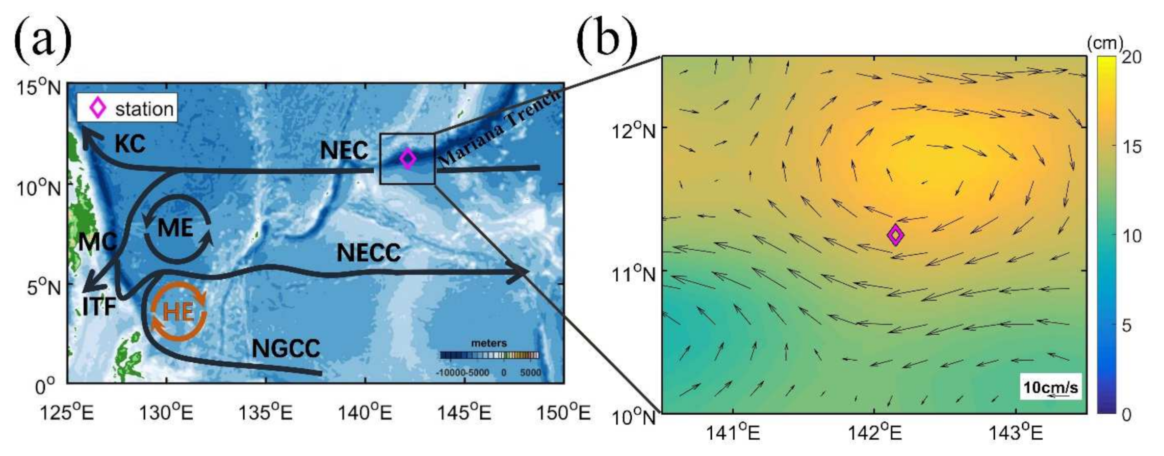
:1. Introduction
2. Observations and Methods
3. Meteorological and Hydrological Conditions
4. Results
4.1. The Barrier Layer
4.2. Turbulence Characteristics
4.2.1. Evolution of ε in the Mixed Layer
4.2.2. Evolution of ε below the Mixed Layer
4.2.3. Shear and Stratification
4.3. Double Diffusion
5. Discussion and Conclusions
Supplementary Materials
Author Contributions
Funding
Data Availability Statement
Acknowledgments
Conflicts of Interest
Abbreviations
| ε | Turbulent Kinetic Energy Dissipation Rate |
| WPNEC | Western Pacific North Equatorial Current |
| ML | Mixed Layer |
| NEC | North Equatorial Current |
| KC | Kuroshio Current |
| MC | Mindanao Current |
| NPTW | North Pacific Tropical Water |
| BL | Barrier Layers |
| IL | Isothermal Layer |
| TL | Transition Layer |
| MSP | Microstructure Profile |
| LT | Local Time |
| LADCP | Lowered Acoustic Doppler Current Profiler |
| CTD | Conductivity, Temperature, Depth |
| AE | Anticyclonic Eddy |
| TSW | Tropical Surface Water |
| ITCZ | Intertropical Convergence Zone |
References
- Crawford, W.R.; Osborn, T.R. Turbulence in the Equatorial Pacific Ocean, Pacific Marine Science Report 81-1; Institute of Ocean Sciences: Sidney, BC, Canada, 1981. [Google Scholar]
- Dewar, W.K. Simple models of stratification. J. Phys. Oceanogr. 1991, 21, 1762–1779. [Google Scholar] [CrossRef] [Green Version]
- Munk, W.; Wunsch, C. Abyssal recipes II: Energetics of tidal and wind mixing. Deep-Sea Res. Pt. I 1998, 45, 1977–2010. [Google Scholar] [CrossRef]
- D’Asaro, E.A. Turbulent Vertical Kinetic Energy in the Ocean Mixed Layer. J. Phys. Oceanogr. 2001, 31, 3530–3537. [Google Scholar] [CrossRef]
- Lien, R.-C.; D’Asaro, E.A.; McPhaden, M.J. Internal Waves and Turbulence in the Upper Central Equatorial Pacific: Lagrangian and Eulerian Observations. J. Phys. Oceanogr. 2002, 32, 2619–2639. [Google Scholar] [CrossRef] [Green Version]
- Large, W.G.; Mcwilliams, J.C.; Doney, S.C. Oceanic Vertical Mixing—A Review and a Model with a Nonlocal Boundary-Layer Parameterization. Rev. Geophys. 1994, 32, 363–403. [Google Scholar] [CrossRef] [Green Version]
- McWilliams, J.C. Modeling the oceanic general circulation. Annu. Rev. Fluid Mech. 1996, 28, 215–248. [Google Scholar] [CrossRef]
- Langmuir, I. Surface motion of water induced by wind. Science 1938, 87, 119–123. [Google Scholar] [CrossRef] [PubMed]
- Craik, A.D.D.; Leibovich, S. Rational Model for Langmuir Circulations. J. Fluid Mech. 1976, 73, 401–426. [Google Scholar] [CrossRef] [Green Version]
- Skyllingstad, E.D.; Denbo, D.W. An Ocean Large-Eddy Simulation of Langmuir Circulations and Convection in the Surface Mixed-Layer. J. Geophys. Res. Oceans 1995, 100, 8501–8522. [Google Scholar] [CrossRef]
- McWilliams, J.C.; Sullivan, P.P.; Moeng, C.H. Langmuir turbulence in the ocean. J. Fluid Mech. 1997, 334, 1–30. [Google Scholar] [CrossRef] [Green Version]
- Belcher, S.E.; Grant, A.L.M.; Hanley, K.E.; Fox-Kemper, B.; van Roekel, L.; Sullivan, P.P.; Large, W.G.; Brown, A.; Hines, A.; Calvert, D.; et al. A global perspective on Langmuir turbulence in the ocean surface boundary layer. Geophys. Res. Lett. 2012, 39. [Google Scholar] [CrossRef] [Green Version]
- Fox-Kemper, B.; Danabasoglu, G.; Ferrari, R.; Griffies, S.M.; Hallberg, R.W.; Holland, M.M.; Maltrud, M.E.; Peacock, S.; Samuels, B.L. Parameterization of mixed layer eddies. III: Implementation and impact in global ocean climate simulations. Ocean. Model. 2011, 39, 61–78. [Google Scholar] [CrossRef] [Green Version]
- Furue, R.; Jia, Y.; McCreary, J.P.; Schneider, N.; Richards, K.J.; Müller, P.; Cornuelle, B.D.; Avellaneda, N.M.; Stammer, D.; Liu, C.; et al. Impacts of regional mixing on the temperature structure of the equatorial Pacific Ocean. Part 1: Vertically uniform vertical diffusion. Ocean. Model. 2015, 91, 91–111. [Google Scholar] [CrossRef] [Green Version]
- Richards, K.J.; Kashino, Y.; Natarov, A.; Firing, E. Mixing in the western equatorial Pacific and its modulation by ENSO. Geophys. Res. Lett. 2012, 39. [Google Scholar] [CrossRef]
- Wyrtki, K. The Thermohaline Circulation in Relation to the General Circulation in the Oceans. Deep. Sea Res. 1961, 8, 39–64. [Google Scholar] [CrossRef]
- Nitani, H. Beginning of the Kuroshio. Kuroshio: Physical Aspects of the Japan Current; Stommel, H., Oshida, K.Y., Eds.; University of Washington Press: Seattle, WA, USA, 1972; pp. 129–163. [Google Scholar]
- Qiu, B.; Lukas, R. Seasonal and interannual variability of the North Equatorial Current, the Mindanao Current, and the Kuroshio along the Pacific western boundary. J. Geophys. Res. Oceans 1996, 101, 12315–12330. [Google Scholar] [CrossRef]
- Qu, T.D.; Mitsudera, H.; Yamagata, T. On the western boundary currents in the Philippine Sea. J. Geophys. Res. Oceans 1998, 103, 7537–7548. [Google Scholar] [CrossRef]
- Fine, R.A.; Lukas, R.; Bingham, F.M.; Warner, M.J.; Gammon, R.H. The western equatorial pacific—A water mass crossroads. J. Geophys. Res.-Oceans 1994, 99, 25063–25080. [Google Scholar] [CrossRef] [Green Version]
- Li, Y.; Wang, F. Spreading and salinity change of North Pacific Tropical Water in the Philippine Sea. J. Oceanogr. 2012, 68, 439–452. [Google Scholar] [CrossRef]
- Qu, T.D.; Mitsudera, H.; Yamagata, T. A climatology of the circulation and water mass distribution near the Philippine coast. J. Phys. Oceanogr. 1999, 29, 1488–1505. [Google Scholar] [CrossRef] [Green Version]
- Suga, T.; Kato, A.; Hanawa, K. North Pacific Tropical Water: Its climatology and temporal changes associated with the climate regime shift in the 1970s. Prog. Oceanogr. 2000, 47, 223–256. [Google Scholar] [CrossRef]
- Xie, L.; Tian, J.; Hu, D.; Wang, F. A quasi-synoptic interpretation of water mass distribution and circulation in the western North Pacific II: Circulation. Chin. J. Oceanol. Limnol. 2009, 27, 955–965. [Google Scholar] [CrossRef]
- Lukas, R.; Lindstrom, E. The Mixed Layer of the Western Equatorial Pacific-Ocean. J. Geophys. Res. Oceans 1991, 96, 3343–3357. [Google Scholar] [CrossRef]
- Sprintall, J.; Tomczak, M. Evidence of the barrier layer in the surface layer of the tropics. J. Geophys. Res. 1992, 97, 7305–7316. [Google Scholar] [CrossRef] [Green Version]
- Gu, D.F.; Philander, S.G.H.; McPhaden, M.J. The seasonal cycle and its modulation in the eastern tropical Pacific Ocean. J. Phys. Oceanogr. 1997, 27, 2209–2218. [Google Scholar] [CrossRef] [Green Version]
- Vialard, J.; Delecluse, P. An OGCM study for the TOGA decade. Part II: Barrier-layer formation and variability. J. Phys. Oceanogr. 1998, 28, 1089–1106. [Google Scholar] [CrossRef]
- Zhang, R.H.; Rothstein, L.M.; Busalacchi, A.J. Origin of upper-ocean warming and El Nino change on decadal scales in the tropical Pacific Ocean. Nature 1998, 391, 879–883. [Google Scholar] [CrossRef]
- Schneider, N. The response of tropical climate to the equatorial emergence of spiciness anomalies. J. Clim. 2004, 17, 1083–1095. [Google Scholar] [CrossRef]
- Sasaki, H.; Xie, S.P.; Taguchi, B.; Nonaka, M.; Masumoto, Y. Seasonal variations of the Hawaiian Lee Countercurrent induced by the meridional migration of the trade winds. Ocean Dynam 2010, 60, 705–715. [Google Scholar] [CrossRef]
- Katsura, S.; Oka, E.; Qiu, B.; Schneider, N. Formation and Subduction of North Pacific Tropical Water and Their Interannual Variability. J. Phys. Oceanogr. 2013, 43, 2400–2415. [Google Scholar] [CrossRef] [Green Version]
- Price, J.F.; Weller, R.A.; Pinkel, R. Diurnal cycling: Observations and models of the upper ocean response to diurnal heating, cooling, and wind mixing. J. Geophys. Res. 1986, 91, 8411–8427. [Google Scholar] [CrossRef] [Green Version]
- Gordon, C.; Corry, R.A. A Model Simulation of the Seasonal Cycle in the Tropical Pacific-Ocean Using Climatological and Modeled Surface Forcing. J. Geophys. Res. Oceans 1991, 96, 847–864. [Google Scholar] [CrossRef]
- Sato, K.; Suga, T.; Hanawa, K. Barrier layer in the North Pacific subtropical gyre. Geophys. Res. Lett. 2004, 31. [Google Scholar] [CrossRef]
- Edwards, N.R.; Richards, K.J. Nonlinear double-diffusive intrusions at the equator. J. Mar. Res. 2004, 62, 233–259. [Google Scholar] [CrossRef]
- Richards, K.; Banks, H. Characteristics of interleaving in the western equatorial Pacific. J. Geophys. Res. Oceans 2002, 107, 24-1–24-12. [Google Scholar] [CrossRef]
- Lee, C.; Chang, K.I.; Lee, J.H.; Richards, K.J. Vertical mixing due to double diffusion in the tropical western Pacific. Geophys. Res. Lett. 2014, 41, 7964–7970. [Google Scholar]
- Schmitt, R.W.; Perkins, H.; Boyd, J.D.; Stalcup, M.C. C-salt—An investigation of the thermohaline staircase in the western tropical north-atlantic. Deep-Sea Res. 1987, 34, 1655–1665. [Google Scholar] [CrossRef]
- Tsuchiya, M.; Talley, L.D. A Pacific hydrographic section at 88 degrees W: Water-property distribution. J. Geophys. Res.-Oceans 1998, 103, 12899–12918. [Google Scholar] [CrossRef] [Green Version]
- Wong, A.P.S.; Johnson, G.C. South Pacific Eastern Subtropical Mode Water. J. Phys. Oceanogr. 2003, 33, 1493–1509. [Google Scholar] [CrossRef]
- McCreary, J.P.; Lu, P. Interaction between the subtropical and equatorial ocean circulations—The subtropical cell. J. Phys. Oceanogr. 1994, 24, 466–497. [Google Scholar]
- Moum, J.N.; Caldwell, D.R. Local Influences on Shear-Flow Turbulence in the Equatorial Ocean. Science 1985, 230, 315–316. [Google Scholar] [CrossRef] [PubMed]
- Gregg, M.C.; Peters, H.; Wesson, J.C.; Oakey, N.S.; Shay, T.J. Intensive Measurements of Turbulence and Shear in the Equatorial Undercurrent. Nature 1985, 318, 140–144. [Google Scholar] [CrossRef]
- Visbeck, M. Deep velocity profiling using lowered acoustic Doppler current profilers: Bottom track and inverse solutions. J. Atmos. Ocean. Technol. 2002, 19, 794–807. [Google Scholar] [CrossRef]
- Thurnherr, A. How to Process LADCP Data with the LDEO Software, Versions IX.7–IX.13; Lamont Doherty Earth Observatory: New York, NY, USA, 2018; Volume 5. [Google Scholar]
- Roget, E.; Lozovatsky, I.; Sanchez, X.; Figueroa, M. Microstructure measurements in natural waters: Methodology and applications. Prog. Oceanogr. 2006, 70, 126–148. [Google Scholar] [CrossRef]
- Osborn, T.R. Estimates of the local-rate of vertical diffusion from dissipation measurements. J. Phys. Oceanogr. 1980, 10, 83–89. [Google Scholar] [CrossRef] [Green Version]
- Berrisford, P.; Kållberg, P.; Kobayashi, S.; Dee, D.; Uppala, S.; Simmons, A.J.; Poli, P.; Sato, H. Atmospheric conservation properties in ERA-Interim. Q. J. R. Meteorol. Soc. 2011, 137, 1381–1399. [Google Scholar] [CrossRef]
- Shay, T.J.; Gregg, M.C. Convectively driven turbulent mixing in the upper ocean. J. Phys. Oceanogr. 1986, 16, 1777–1798. [Google Scholar] [CrossRef]
- Fairall, C.W.; Bradley, E.F.; Rogers, D.P.; Edson, J.B.; Young, G.S. Bulk parameterization of air-sea fluxes for Tropical Ocean Global Atmosphere Coupled Ocean Atmosphere Response Experiment. J. Geophys. Res. Oceans 1996, 101, 3747–3764. [Google Scholar] [CrossRef]
- You, Y.Z. Salinity Variability and Its Role in the Barrier-Layer Formation during Toga-Coare. J. Phys. Oceanogr. 1995, 25, 2778–2807. [Google Scholar] [CrossRef] [Green Version]
- Chu, P.C.; Liu, Q.Y.; Jia, Y.L.; Fan, C.W. Evidence of a barrier layer in the Sulu and Celebes Seas. J. Phys. Oceanogr. 2002, 32, 3299–3309. [Google Scholar] [CrossRef] [Green Version]
- Ferrari, R.; Boccaletti, G. Eddy-mixed layer interactions in the ocean. Oceanography 2004, 17, 12–21. [Google Scholar] [CrossRef] [Green Version]
- Turner, J.S. Buoyancy Effects in Fluids; Cambridge University Press: Cambridge, UK, 1973. [Google Scholar]
- Ruddick, B.R. A practical indicator of the stability of the water column to double-diffusive activity. Deep-Sea Res. 1983, 30, 1105–1107. [Google Scholar] [CrossRef]
- Mcdougall, T.J.; Thorpe, S.A.; Gibson, C.H. Small-Scale Turbulence and Mixing in the Ocean: A Glossary; Elsevier: Amsterdam, The Netherlands, 1988; Volume 46, pp. 3–9. [Google Scholar]
- Gregg, M.C. Mixing in the Thermohaline Staircase East of Barbados. Small-Scale Turbulence and Mixing in the Ocean. In Proceedings of the 19th International Liege Colloquium on Ocean Hydrodynamics, Liege, Belgium, 4–8 May 1987; pp. 453–470. [Google Scholar]
- Inoue, R.; Yamazaki, H.; Wolk, F.; Kono, T.; Yoshida, J. An Estimation of Buoyancy Flux for a Mixture of Turbulence and Double Diffusion. J. Phys. Oceanogr. 2007, 37, 611–624. [Google Scholar] [CrossRef]
- Schmitt, R.W. Form of the temperature–salinity relationship in the central water: Evidence for double-diffusive mixing. J. Phys. Oceanogr. 1981, 11, 1015–1026. [Google Scholar] [CrossRef] [Green Version]
- Merryfield, W.J.; Holloway, G.; Gargett, A.E. A global ocean model with double-diffusive mixing. J. Phys. Oceanogr. 1999, 29, 1124–1142. [Google Scholar] [CrossRef]
- Callaghan, A.H.; Ward, B.; Vialard, J. Influence of surface forcing on near-surface and mixing layer turbulence in the tropical Indian Ocean. Deep-Sea Res. Part I 2014, 94, 107–123. [Google Scholar] [CrossRef]
- Tsuchiya, M. Upper waters of the intertropical Pacific Ocean. Johns Hopkins Oceanogr. Stud. 1968, 4, 50. [Google Scholar]
- Veronis, G. On properties of seawater defined by temperature, salinity, and pressure. J. Mar. Res. 1972, 30, 227–255. [Google Scholar] [CrossRef]
- Munk, W.; Worcester, P.; Zachariasen, F. Scattering of Sound by Internal Wave Currents—The Relation to Vertical Momentum Flux. J. Phys. Oceanogr. 1981, 11, 442–454. [Google Scholar] [CrossRef] [Green Version]
- Tomczak, M. Salinity Variability in the Surface-Layer of the Tropical Western Pacific-Ocean. J. Geophys. Res. Oceans 1995, 100, 20499–20515. [Google Scholar] [CrossRef]
- Woods, J.D.; Barkmann, W. A Lagrangian Mixed Layer Model of Atlantic 18-Degrees-C Water Formation. Nature 1986, 319, 574–576. [Google Scholar] [CrossRef]
- Brainerd, K.E.; Gregg, M.C. Surface Mixed and Mixing Layer Depths. Deep-Sea Res. Part I 1995, 42, 1521–1543. [Google Scholar] [CrossRef]
- Hughes, K.G.; Moum, J.N.; Shroyer, E.L. Evolution of the velocity structure in the diurnal warm layer. J. Phys. Oceanogr. 2020, 50, 615–631. [Google Scholar] [CrossRef]
- Brainerd, K.E.; Gregg, M.C. Diurnal restratification and turbulence in the oceanic surface mixed layer: 1. Observations. J. Geophys. Res. 1993, 98, 22645–22656. [Google Scholar] [CrossRef]
- Gargett, A.E. Ocean Turbulence. Annu. Rev. Fluid Mech. 1989, 21, 419–451. [Google Scholar] [CrossRef]
- Zhang, Z.W.; Qiu, B.; Tian, J.; Zhao, W.; Huang, X. Latitude-dependent finescale turbulent shear generations in the Pacific tropical-extratropical upper ocean. Nat. Commun. 2018, 9, 4086. [Google Scholar] [CrossRef]
- Kantha, L.H.; Clayson, C.A. An Improved Mixed-Layer Model for Geophysical Applications. J. Geophys. Res. Oceans 1994, 99, 25235–25266. [Google Scholar] [CrossRef]
- Johnston, T.M.S.; Rudnick, D.L. Observations of the transition layer. J. Phys. Oceanogr. 2009, 39, 780. [Google Scholar] [CrossRef]
- Rahter, B.A. Turbulent Dissipation Properties of the Midlatitude Mixed Layer/Thermocline Transition Layer. Master’s Thesis, Florida State University, Tallahassee, FL, USA, 2010; p. 60. [Google Scholar]
- Sun, O.M.; Jayne, S.R.; Polzin, K.L.; Rahter, B.A.; Laurent, L.C.S. Scaling Turbulent Dissipation in the Transition Layer. J. Phys. Oceanogr. 2013, 43, 2475–2489. [Google Scholar] [CrossRef] [Green Version]
- Gregg, M.C.; Sanford, T.B. The Dependence of Turbulent Dissipation on Stratification in a Diffusively Stable Thermocline. J. Geophys. Res. Oceans 1988, 93, 12381–12392. [Google Scholar] [CrossRef]
- Polzin, K.L.; Toole, J.M.; Schmitt, R.W. Finescale Parameterizations of Turbulent Dissipation. J. Phys. Oceanogr. 1995, 25, 306–328. [Google Scholar] [CrossRef] [Green Version]
- Polzin, K.L.; Oakey, N.S.; Toole, J.M.; Schmitt, R.W. Fine structure and microstructure characteristics across the northwest atlantic subtropical front. J. Geophys. Res. Ocean. 1996, 101, 14111–14121. [Google Scholar] [CrossRef]
- Avicola, G.S.; Moum, J.N.; Perlin, A.; Levine, M.D. Enhanced turbulence due to the superposition of internal gravity waves and a coastal upwelling jet. J. Geophys. Res. 2007, 112. [Google Scholar] [CrossRef] [Green Version]
- Kara, A.B.; Rochford, P.A.; Hurlburt, H.E. Mixed layer depth variability over the global ocean. J. Geophys. Res. 2003, 108, 3079. [Google Scholar] [CrossRef] [Green Version]
- de Boyer Montégut, C.; Madec, G.; Fischer, A.S.; Lazar, A.; Iudicone, D. Mixed layer depth over the global ocean: An examination of profile data and a profile-based climatology. J. Geophys. Res. 2004, 109, C12003. [Google Scholar] [CrossRef]
- Yeager, S.; Large, W. Observational Evidence of Winter Spice Injection. J. Phys. Oceanogr. 2007, 37, 2895–2919. [Google Scholar] [CrossRef] [Green Version]
- Yamazaki, H. Stratified turbulence near a critical dissipation rate. J. Phys. Oceanogr. 1990, 20, 1583–1598. [Google Scholar] [CrossRef] [Green Version]


| N | |||||||
|---|---|---|---|---|---|---|---|
| (m/s) | (W kg−1) | (m) | (m) | (m) | (W m−2) | ||
| Period I | 7.84 | −2.40 × 10⁻⁷ | −33.19 | 96.71 | 11.19 | −515.89 | 18 |
| Period II | 9.34 | 1.42 × 10⁻⁷ | 27.22 | 95.97 | 12.27 | 304.71 | 11 |
| Period III | 9.29 | 1.39 × 10⁻⁷ | 28.29 | 96.53 | 6.58 | 297.97 | 12 |
| Period IV | 8.84 | −3.32 × 10⁻⁷ | −20.39 | 94.08 | 9.67 | −741.04 | 12 |
Publisher’s Note: MDPI stays neutral with regard to jurisdictional claims in published maps and institutional affiliations. |
© 2022 by the authors. Licensee MDPI, Basel, Switzerland. This article is an open access article distributed under the terms and conditions of the Creative Commons Attribution (CC BY) license (https://creativecommons.org/licenses/by/4.0/).
Share and Cite
Yang, W.; Zhou, H.; Wang, Y.; Liu, J.; Liu, H.; Liu, C.; Dewar, W. Direct Measurements of Turbulence in the Upper Western Pacific North Equatorial Current over a 25-h Period. Sensors 2022, 22, 1167. https://doi.org/10.3390/s22031167
Yang W, Zhou H, Wang Y, Liu J, Liu H, Liu C, Dewar W. Direct Measurements of Turbulence in the Upper Western Pacific North Equatorial Current over a 25-h Period. Sensors. 2022; 22(3):1167. https://doi.org/10.3390/s22031167
Chicago/Turabian StyleYang, Wenlong, Hui Zhou, Yonggang Wang, Juan Liu, Hengchang Liu, Chenglong Liu, and William Dewar. 2022. "Direct Measurements of Turbulence in the Upper Western Pacific North Equatorial Current over a 25-h Period" Sensors 22, no. 3: 1167. https://doi.org/10.3390/s22031167