The MCM, which is defined in Supplement 1 to the Guide to the expression of Uncertainty in Measurements (GUM) [
15], was used to determine the estimate and the uncertainty of the measurement of the leakage flow, which could be obtained indirectly from the measurements of the CO
2 concentration levels and of the source of CO
2 in the cabin. The leakage flow is the product between the air exchange rate (AER) and the cabin volume (
); in essence, it is the fresh air flow that enters the cabin, which is also equal to the air flow exhausted by the cabin. The model that correlates the leakage flow (
) to the mean CO
2 concentration (
) in the cabin volume is this mass balance equation:
where
is the CO
2 concentration level in the external ambient conditions,
is the source of CO
2, and
is the time instant. With the kind of sensors described in
Section 2, the measurable quantities are
,
, and
. Thus, in this equation there are 2 unknowns; these are the leakage flow
and the cabin volume
. According to Jung [
16], when a vehicle is motionless, and the wind speed is therefore zero, and the ventilation fan is off, the leakage flow is negligible and the mass balance Equation (5) for the CO
2 becomes, after integrating in time:
where
is the initial value of the CO
2 concentration in the cabin. In this particular condition, we obtain a linear equation with only one unknown, which is the cabin volume. Therefore, from Equation (6), considering two time instants,
and
, it is possible to find
:
where
and
are the mean CO
2 concentration levels in the cabin volume, respectively, at time
and
.
has been substituted with
, where
is the CO
2 mass flow injected into the cabin and measured with the mass flow meter. A test was performed where the CO
2 concentration levels were measured with the cabin in this condition. With the results obtained from the measurements at time
and
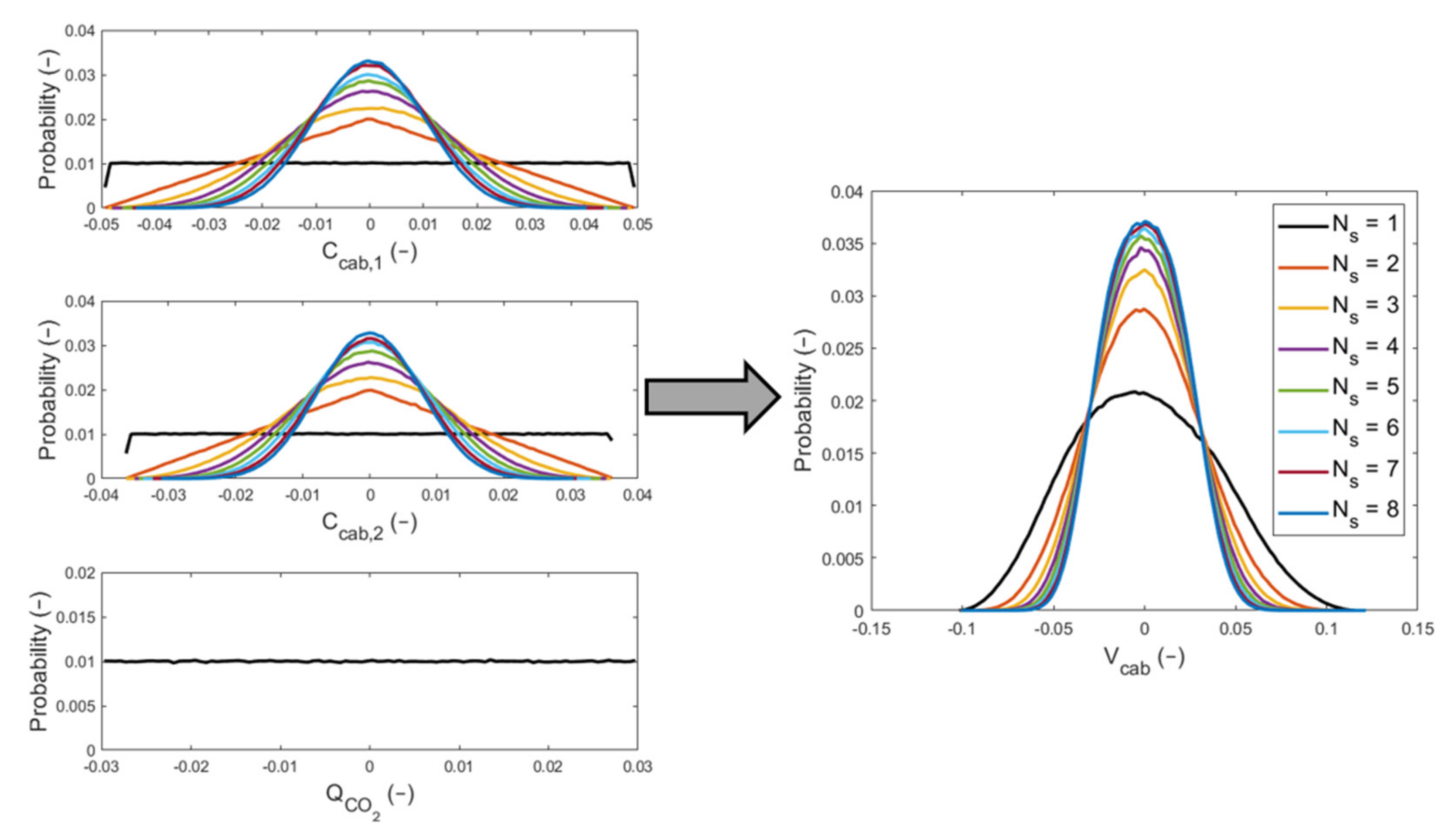
, we applied the MCM to find the mean and the standard deviation estimations of the cabin volume. We defined
to be equal to 3 × 10
6, the number of Monte Carlo trials. Thus, we generated a sequence of
values for each input quantity (
,
and
) by performing
random sampling from their probability distributions. Consecutively, we obtained a sequence of
values for
from the calculation of Equation (7) for the
trials. We did not corrupt the MCM with the quantities
and
because the error on the timestamp is negligible with respect to the other measurements. The variables
and
are obtained from the mean value of the measurements made by the sensors (
and
, where
is the sensor counter) placed inside the cabin. The reason is that Equation (7) is a lumped-parameter model; so, only one value of the CO
2 concentration level is considered for the entire cabin. For each input quantity, we considered a rectangular distribution, which means the error is uniformly distributed inside the interval of accuracy of each sensor, as given by the datasheet. The output signals of both the CO
2 sensors and the mass flow meter were already processed by their on-board microchips; the microprocessors (Arduino 2560 Mega and STM32F411RE) received a message of zeros and ones from the slave devices. Therefore, no other errors were added to the ones specified by the datasheets of the sensors. The choice of considering the error as uniformly distributed is motivated by the fact that the manufacturer of the sensors did not provide a PDF (Probability Density Function) associated with the accuracy, but only an interval. As stated in the GUM [
22], if the only available information regarding a quantity
is a lower limit
and un upper limit
with
, then, according to the principle of maximum entropy, a rectangular distribution
over the interval
would be assigned to
. Let us define
as a generic input quantity with
and
as its lower and upper limits, respectively. We can write the generic element
of the corrupted sequence
as:
where
is the element counter and
is a random draw from the standard rectangular distribution whose lower and upper limits are 0 and 1, respectively. As
(
) was calculated as the mean value of the measurements made in
spots inside the cabin, the element of the corrupted sequence
can be written as:
where
and
are the lower and upper limits for
(CO
2 measurement in the spot number
). The same formula can also be written for
. Substituting the input quantities in Equation (7) with the respective
corrupted values, we obtained a sequence of
corrupted elements
. Finally, from these
samples of the cabin volume obtained through the MCM, we could calculate the estimation of the mean value and of the standard deviation for the cabin volume:
and
.
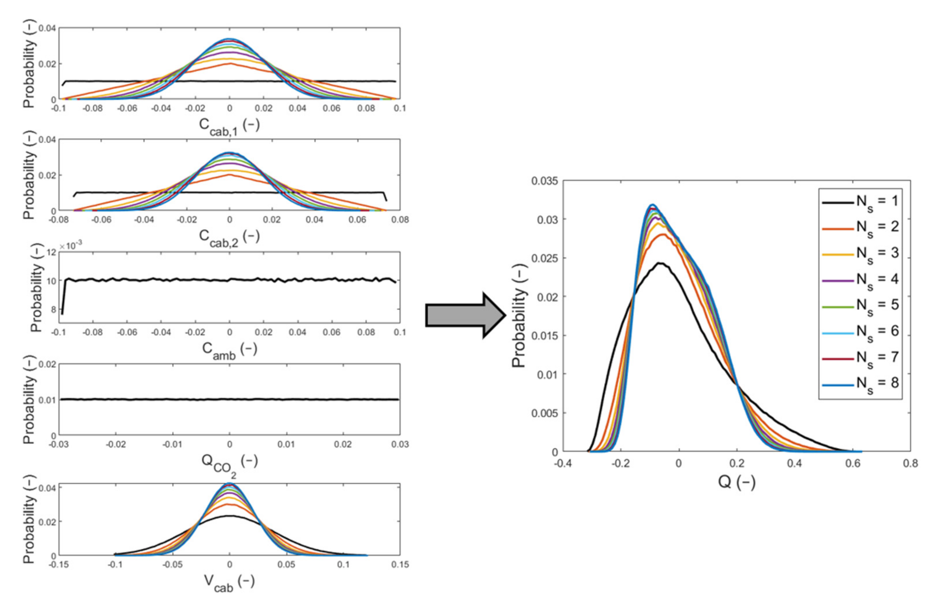
The same procedure used for the cabin volume was now repeated to find the estimate and the coverage interval for the leakage flow
. This time, we performed a test with the ventilation fan speed fixed at 50% of its maximum, where the CO
2 concentration levels were measured in the various spots inside the cabin and in the external ambient conditions; moreover, the CO
2 mass flow injected into the cabin was measured. We used rectangular distributions for the input quantities
,
,
, and
. As shown in
Section 3.3, a Gaussian distribution was obtained for
; so, the element of the corrupted sequence
was calculated at each trial of the MCM as:
where
is a random draw from the standard Gaussian distribution that has the best estimate equal to 0 and the variance equal to 1. Finally, substituting in Equation (10) the input quantities with their corrupted sequences
,
,
,
, and
, a sequence
of
elements was obtained by solving Equation (10) numerically. From these
samples of the leakage flow, we could calculate the mean value (
) and the 95% coverage interval for
.
The code used to apply the MCM to Equations (7) and (10), was written in the Matlab environment. Moreover, to calculate the mean value and standard deviation of a variable, the Matlab tools mean and std were used, respectively. Another Matlab tool, fzero, was utilized to find numerically the value of that solves Equation (10) at each Monte Carlo trial. Finally, the probability distribution of each variable was obtained thanks to the Matlab tool histogram.


 ,
, 


