
Underwater Energy Harvesting to Extend Operation Time of Submersible Sensors

 ,
,  , ,
, ,  ,
,  and
and 
Abstract
:
1. Introduction
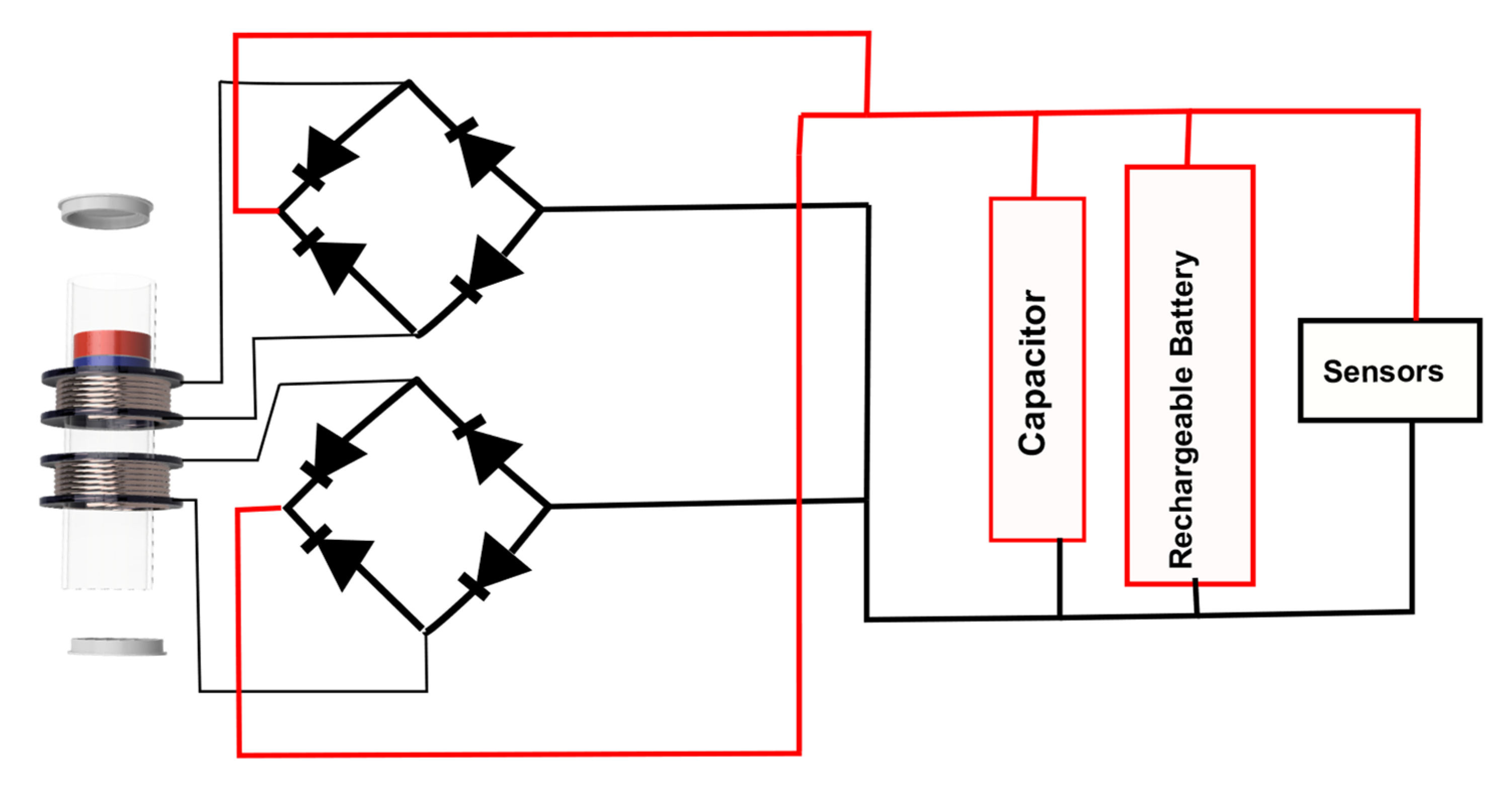
2. Energy Harvesting System Description
3. Materials and Methods
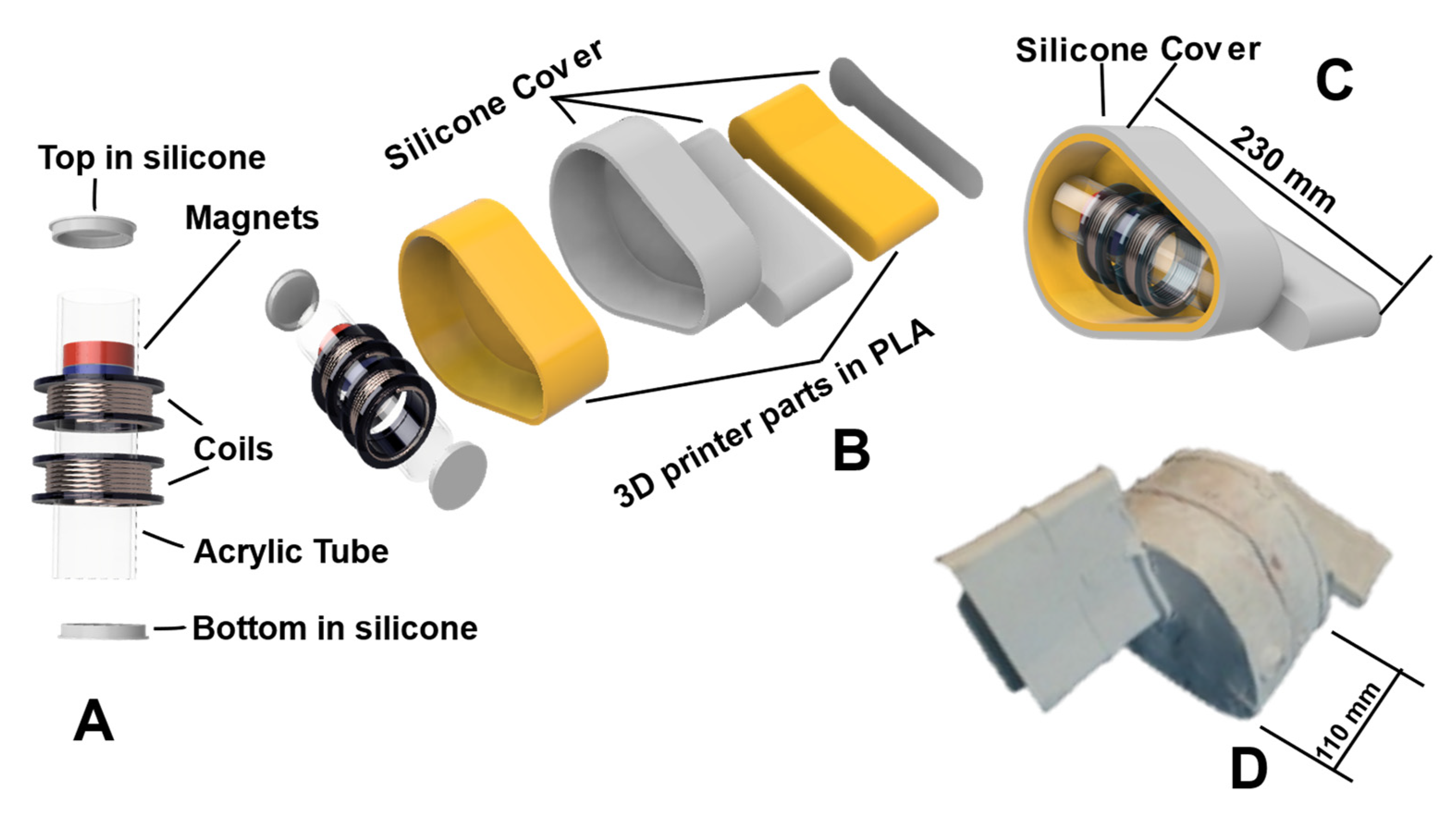
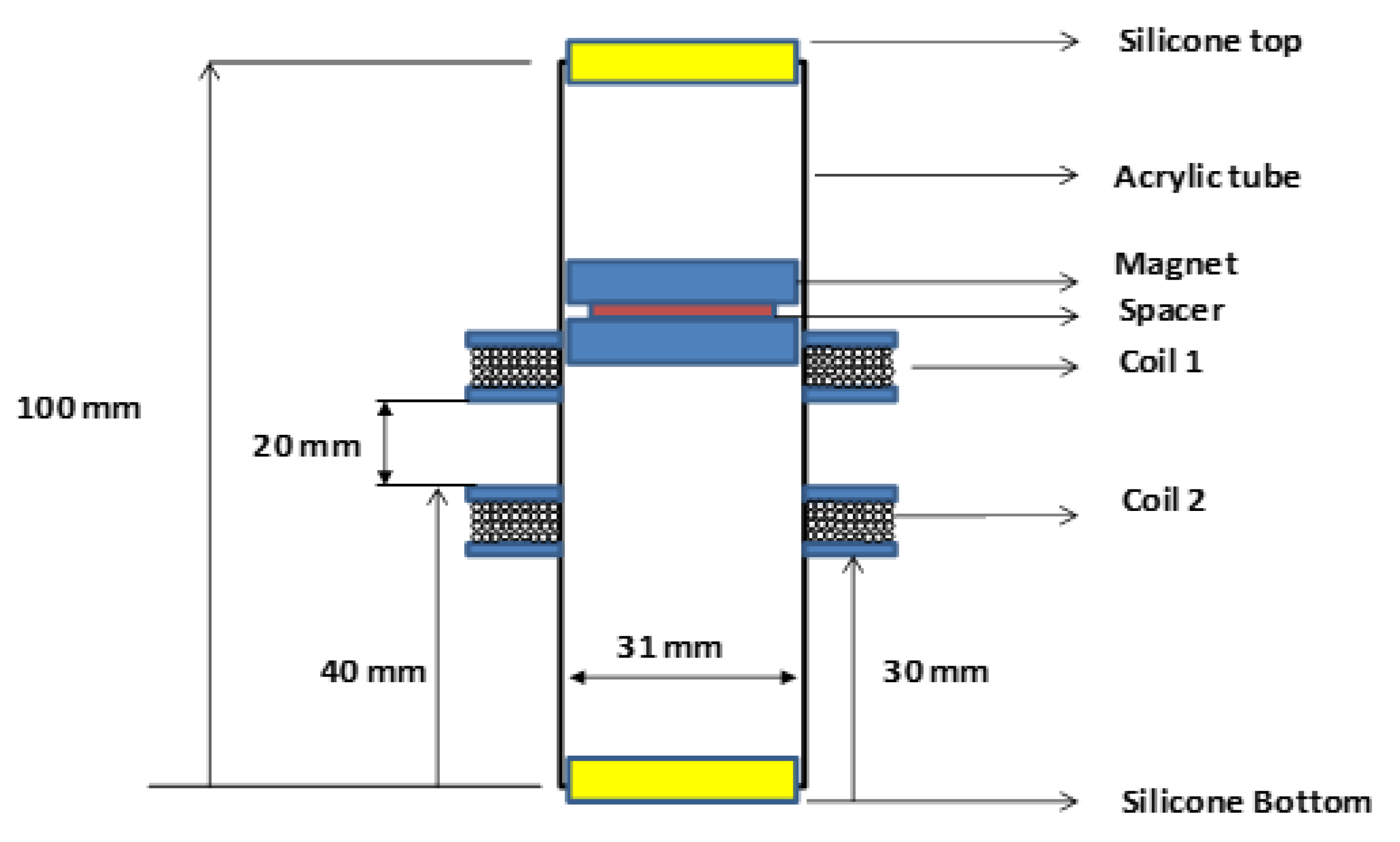
3.1. The LEG Prototype
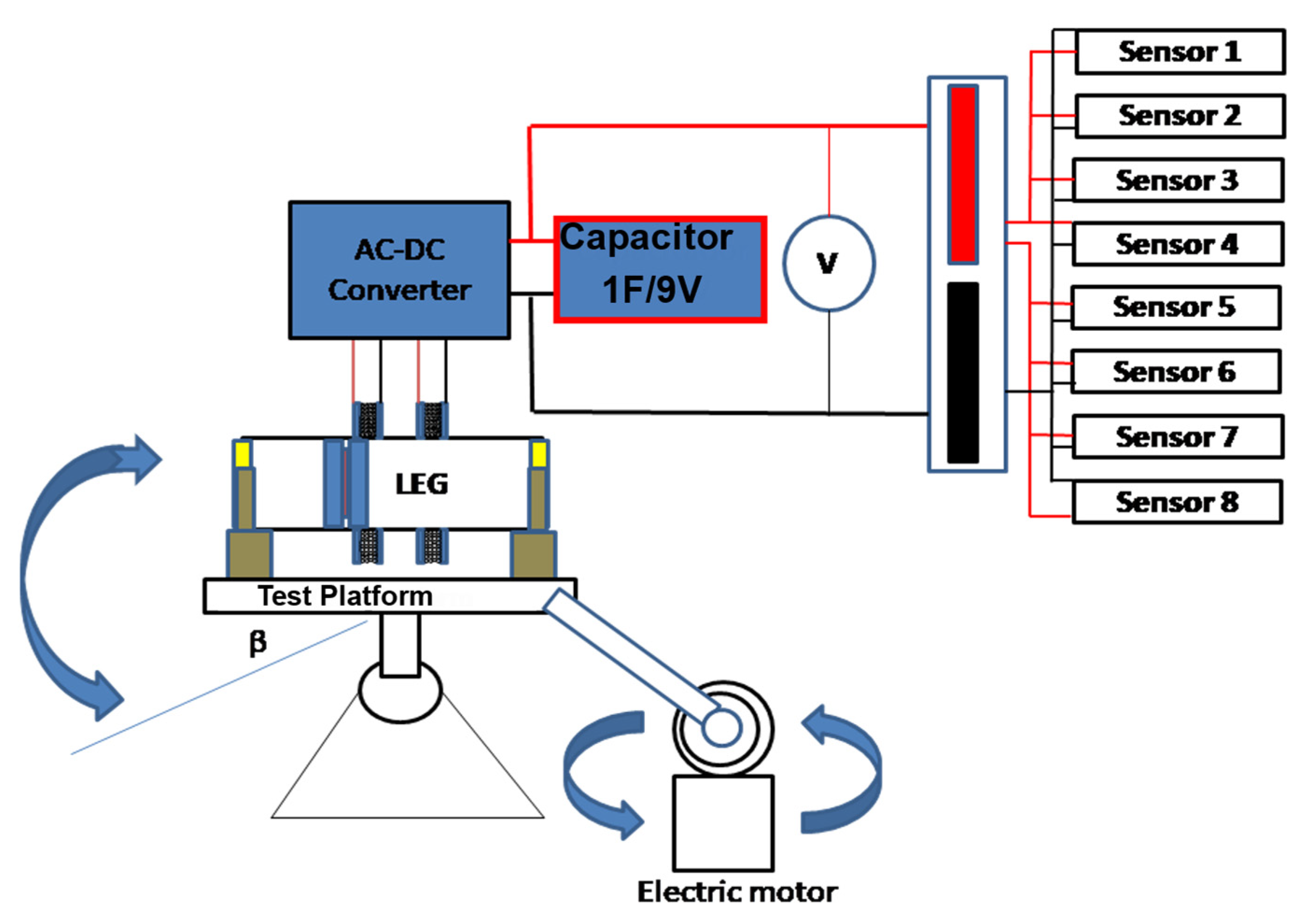
3.2. Methods
3.2.1. Freefall Tests
3.2.2. Load Tests
3.2.3. Frequency Tests
4. Results and Discussion
4.1. Open-Circuit Voltage Output
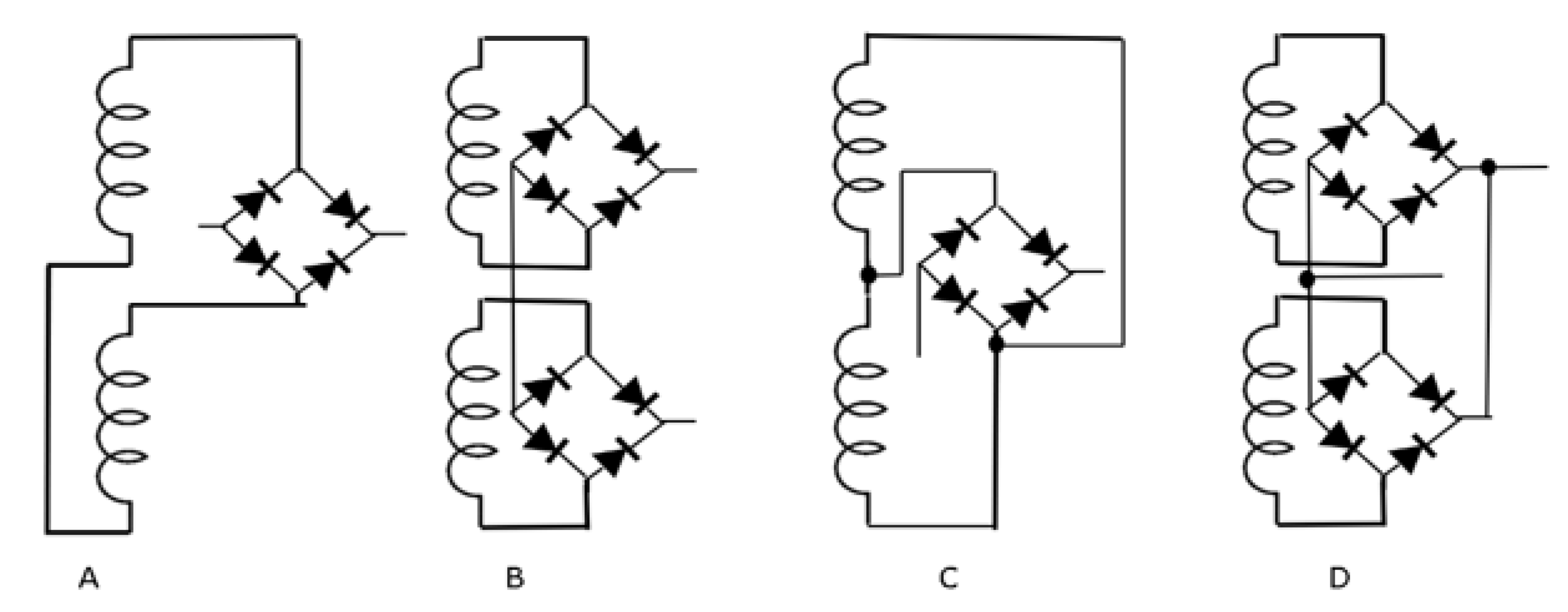
4.1.1. Coils in Series Followed by Rectification
4.1.2. Coils in Series after Rectification
4.1.3. Coils in Parallel Followed by Rectification
4.1.4. Coils in Parallel after Rectification
4.2. Comparison of Results
4.3. Output Power
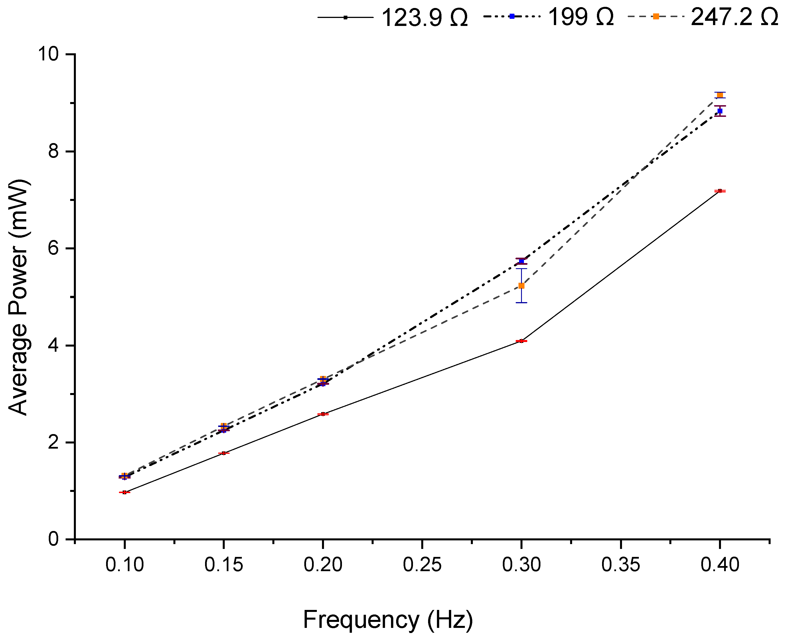
4.3.1. Load Dependence of Output Power
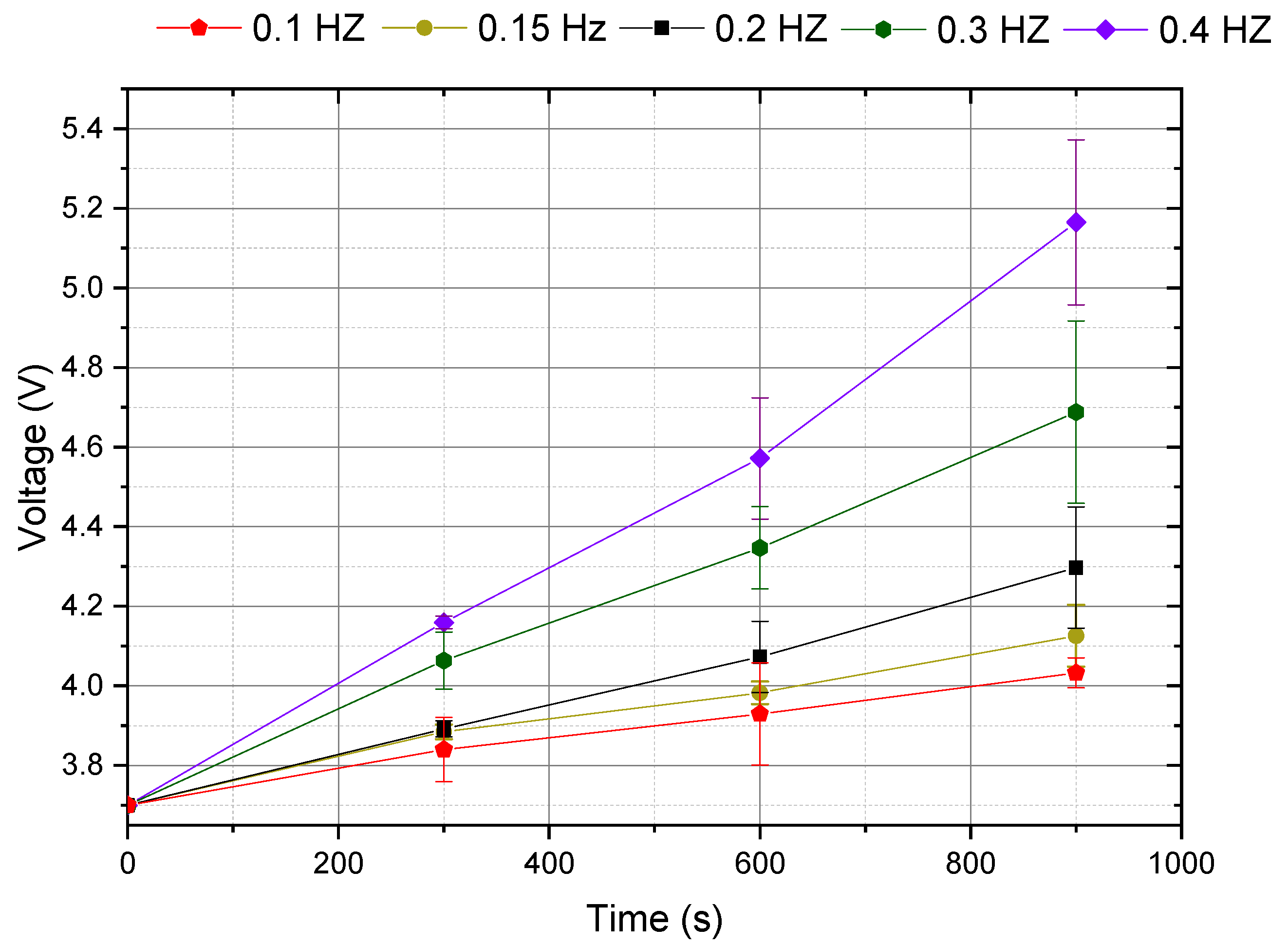
4.3.2. Frequency Dependence of Output Power
5. Conclusions
Author Contributions
Funding
Institutional Review Board Statement
Informed Consent Statement
Data Availability Statement
Acknowledgments
Conflicts of Interest
References
- Martins, M.S.; Barardo, C.; Matos, T.; Gonçalves, L.M.; Cabral, J.; Silva, A.; Jesus, S.M. High Frequency Wide Beam PVDF Ultrasonic Projector for Underwater Communications. In Proceedings of the OCEANS 2017—Aberdeen 2017, Aberdeen, UK, 19–22 June 2017. [Google Scholar] [CrossRef]
- Martins, M.S.; Pinto, N.; Rocha, G.; Cabral, J.; Mendez, S.L. Development of a 1 Mbps low power acoustic modem for underwater communications. In Proceedings of the 2014 IEEE International Ultrasonics Symposium (IUS), Chicago, IL USA, 3–6 September 2014; pp. 2482–2485. [Google Scholar] [CrossRef]
- Nimo, A.; Grgić, D.; Reindl, L.M. Optimization of Passive Low Power Wireless Electromagnetic Energy Harvesters. Sensors 2012, 12, 13636–13663. [Google Scholar] [CrossRef] [PubMed]
- Mariello, M.; Guido, F.; Mastronardi, V.M.; Todaro, M.T.; Desmaële, D.; De Vittorio, M. Nanogenerators for harvesting mechanical energy conveyed by liquids. Nano Energy 2019, 57, 141–156. [Google Scholar] [CrossRef]
- Gilbert, J.M.; Balouchi, F. Comparison of energy harvesting systems for wireless sensor networks. Int. J. Autom. Comput. 2008, 5, 334–347. [Google Scholar] [CrossRef] [Green Version]
- Bixler, G.D.; Bhushan, B. Biofouling: Lessons from nature. Philosophical Transactions of the Royal Society A: Mathematical. Phys. Eng. Sci. 2012, 370, 2381–2417. [Google Scholar] [CrossRef]
- Kiran, M.R.; Farrok, O.; Abdullah-Al-Mamun Md Islam, M.d.R.; Xu, W. Progress in Piezoelectric Material Based Oceanic Wave Energy Conversion Technology. IEEE Access 2020, 8, 146428–146449. [Google Scholar] [CrossRef]
- Xie, X.D.; Wang, Q.; Wu, N. Potential of a piezoelectric energy harvester from sea waves. J. Sound Vib. 2014, 333, 1421–1429. [Google Scholar] [CrossRef]
- Maamer, B.; Boughamoura, A.; Fath El-Bab, A.M.R.; Francis, L.A.; Tounsi, F. A review on design improvements and techniques for mechanical energy harvesting using piezoelectric and electromagnetic schemes. Energy Convers. Manag. 2019, 199, 111973. [Google Scholar] [CrossRef]
- Wang, X.; Niu, S.; Yin, Y.; Yi, F.; You, Z.; Wang, Z.L. Triboelectric Nanogenerator Based on Fully Enclosed Rolling Spherical Structure for Harvesting Low-Frequency Water Wave Energy. Adv. Energy Mater. 2015, 5, 1501467. [Google Scholar] [CrossRef]
- Liu, Y.; Li, S.; Liu, C.; Wang, Y.; Zhou, Y.; Yi, H.; Li, Y.; Chang, H.; Tao, K. Spherical electret generator for water wave energy harvesting by folded structure. In Proceedings of the IECON 2019–45th Annual Conference of the IEEE Industrial Electronics Society, Lisbon, Portugal, 14–17 October 2019; pp. 812–815. [Google Scholar] [CrossRef]
- Wu, Y.; Zeng, Q.; Tang, Q.; Liu, W.; Liu, G.; Zhang, Y.; Wu, J.; Hu, C.; Wang, X. A teeterboard-like hybrid nanogenerator for efficient harvesting of low-frequency ocean wave energy. Nano Energy 2020, 67, 104205. [Google Scholar] [CrossRef]
- Gao, W.; Shao, J.; Sagoe-Crentsil, K.; Duan, W. Investigation on energy efficiency of rolling triboelectric nanogenerator using cylinder-cylindrical shell dynamic model. Nano Energy 2021, 80, 105583. [Google Scholar] [CrossRef]
- Tao, K.; Yi, H.; Yang, Y.; Chang, H.; Wu, J.; Tang, L.; Yang, Z.; Wang, N.; Hu, L.; Fu, Y.; et al. Origami-inspired electret-based triboelectric generator for biomechanical and ocean wave energy harvesting. Nano Energy 2020, 67, 104197. [Google Scholar] [CrossRef]
- Lin, Z.; Zhang, B.; Guo, H.; Wu, Z.; Zou, H.; Yang, J.; Wang, Z.L. Super-robust and frequency-multiplied triboelectric nanogenerator for efficient harvesting water and wind energy. Nano Energy 2019, 64, 103908. [Google Scholar] [CrossRef]
- Zhao, T.; Xu, M.; Xiao, X.; Ma, Y.; Li, Z.; Wang, Z.L. Recent progress in blue energy harvesting for powering distributed sensors in ocean. Nano Energy 2021, 88, 106199. [Google Scholar] [CrossRef]
- Shen, F.; Li, Z.; Guo, H.; Yang, Z.; Wu, H.; Wang, M.; Luo, J.; Xie, S.; Peng, Y.; Pu, H. Recent Advances towards Ocean Energy Harvesting and Self-Powered Applications Based on Triboelectric Nanogenerators. Adv. Electron. Mater. 2021, 7, 2100277. [Google Scholar] [CrossRef]
- Kong, H.; Roussinova, V.; Stoilov, V. Renewable energy harvesting from water flow. Int. J. Environ. Stud. 2019, 76, 84–101. [Google Scholar] [CrossRef]
- Wang, J.; Geng, L.; Ding, L.; Zhu, H.; Yurchenko, D. The state-of-the-art review on energy harvesting from flow-induced vibrations. Appl. Energy 2020, 267, 114902. [Google Scholar] [CrossRef]
- Valizadeh, R.; Abbaspour, M.; Rahni, M.T. A low cost Hydrokinetic Wells turbine system for oceanic surface waves energy harvesting. Renew. Energy 2020, 156, 610–623. [Google Scholar] [CrossRef]
- Soares dos Santos, M.P.; Ferreira, J.A.; Simões, J.A.; Pascoal, R.; Torrão, J.; Xue, X.; Furlani, E.P. Magnetic levitation-based electromagnetic energy harvesting: A semi-analytical non-linear model for energy transduction. Sci. Rep. 2016, 6, 18579. [Google Scholar] [CrossRef]
- Kecik, K.; Mitura, A.; Lenci, S.; Warminski, J. Energy harvesting from a magnetic levitation system. Int. J. Non-Linear Mech. 2017, 94, 200–206. [Google Scholar] [CrossRef]
- Morgado, M.L.; Morgado, L.F.; Silva, N.; Morais, R. Mathematical modelling of cylindrical electromagnetic vibration energy harvesters. Int. J. Comput. Math. 2015, 92, 101–109. [Google Scholar] [CrossRef]
- Bendame, M.; Abdel-Rahman, E. Nonlinear Modeling and Analysis of a Vertical Springless Energy Harvester. MATEC Web Conf. 2012, 1, 01004. [Google Scholar] [CrossRef]
- Glynne-Jones, P.; Tudor, M.J.; Beeby, S.P.; White, N.M. An electromagnetic, vibration-powered generator for intelligent sensor systems. Sensors Actuators A Phys. 2004, 110, 344–349. [Google Scholar] [CrossRef] [Green Version]
- Beeby, S.P.; Torah, R.N.; Tudor, M.J.; Glynne-Jones, P.; O’donnell, T.; Saha, C.R.; Roy, S. A micro electromagnetic generator for vibration energy harvesting. J. Micromech. Microeng. 2007, 17, 1257–1265. [Google Scholar] [CrossRef]
- Silva, N.; Santos, P.; Morais, R.; Frias, C.; Ferreira, J.A.; Ramos, A.; Simões, J.A.O.; Reis, M.C. A Vibration-based Energy Harvesting System for Implantable Biomedical Telemetry Systems. In Proceedings of the International Conference on Biomedical Electronics and Devices, SciTePress—Science and and Technology Publications, Rome, Italy, 26–29 January 2011; pp. 329–332. [Google Scholar] [CrossRef]
- Guo, Q.; Sun, M.; Liu, H.; Ma, X.; Chen, Z.; Chen, T.; Sun, L. Design and experiment of an electromagnetic ocean wave energy harvesting device. In Proceedings of the 2018 IEEE/ASME International Conference on Advanced Intelligent Mechatronics (AIM), Auckland, New Zealand, 9–12 July 2018; pp. 381–384. [Google Scholar] [CrossRef]
- Farrok, O.; Islam, M.; Sheikh, M.; Islam, R. Analysis of the Oceanic Wave Dynamics for Generation of Electrical Energy Using a Linear Generator. J. Energy 2016, 2016, 1–14. [Google Scholar] [CrossRef] [Green Version]
- Chiu, M.-C.; Karkoub, M.; Her, M.-G. Energy harvesting devices for subsea sensors. Renew. Energy 2017, 101, 1334–1347. [Google Scholar] [CrossRef]
- Chiu, M.-C. Two-Magnet Energy Harvesting Devices in Subsea Sensors. DEStech Trans. Environ. Energy Earth Sci. 2019, 63–71. [Google Scholar] [CrossRef]
- Joos, J.; Paul, O. Spherical magnetic energy harvester with three orthogonal coils. In Proceedings of the 2015 IEEE SENSORS, Busan, Korea, 1–4 November 2015; pp. 1–4. [Google Scholar] [CrossRef]
- Park, J.; Bhat, G.; Nk, A.; Geyik, C.S.; Ogras, U.Y.; Lee, H.G. Energy per Operation Optimization for Energy-Harvesting Wearable IoT Devices. Sensors 2020, 20, 764. [Google Scholar] [CrossRef] [Green Version]
- La Rosa, R.; Livreri, P.; Trigona, C.; Di Donato, L.; Sorbello, G. Strategies and Techniques for Powering Wireless Sensor Nodes through Energy Harvesting and Wireless Power Transfer. Sensors 2019, 19, 2660. [Google Scholar] [CrossRef] [Green Version]
- Matos, T.; Faria, C.L.; Martins, M.S.S.; Henriques, R.; Gomes, P.A.A.; Goncalves, L.M.M. Development of a Cost-Effective Optical Sensor for Continuous Monitoring of Turbidity and Suspended Particulate Matter in Marine Environment. Sensors 2019, 19, 4439. [Google Scholar] [CrossRef] [Green Version]
- Faria, C.L.; Martins, M.S.; Lima, R.A.; Goncalves, L.M.; Matos, T. Optimization of an Electromagnetic Generator for Underwater Energy Harvester. In Proceedings of the OCEANS 2019—Marseille, Marseille, France, 17–20 June 2019; pp. 1–6. [Google Scholar] [CrossRef]
- Faria, C.L.; Goncalves, L.M.; Martins, M.S.; Lima, R. Energy Harvesting to Increase the Autonomy of Moored Oceanographic Monitoring Stations. In Proceedings of the 2018 OCEANS—MTS/IEEE Kobe Techno-Oceans (OTO), Kobe, Japan, 28–31 May 2018; pp. 1–5. [Google Scholar] [CrossRef]
- Gonçalves, A.; Luísa Morgado, M.; Filipe Morgado, L.; Silva, N.; Morais, R. Numerical Simulation of Inertial Energy Harvesters using Magnets. In Proceedings of the International Conference on Innovation, Engineering and Entrepreneurship 2019, Braga, Portugal, 17–18 October 2019; pp. 757–763. [Google Scholar] [CrossRef]
- Bernal, A.A.; García, L.L. The modelling of an electromagnetic energy harvesting architecture. Appl. Math. Model. 2012, 36, 4728–4741. [Google Scholar] [CrossRef]
- Ren, H.; Wang, T. Development and modeling of an electromagnetic energy harvester from pressure fluctuations. Mechatronics 2018, 49, 36–45. [Google Scholar] [CrossRef]


| Event | Time (s) | Power (mW) | Energy (mJ) |
|---|---|---|---|
| Sleep mode | 299.99 | 0.96 | 287.99 |
| Reading | 0.01 | 320 | 3.2 |
| Total | 300.00 | 0.97 | 291.1 |
| Type Combination | Theoretical Values (V) | Experimental Values (V) | ||
|---|---|---|---|---|
| Coil A to Coil B | Coil B to Coil A | Coil A to Coil B | Coil B to Coil A | |
| Series followed by rectification | 27.10 | 26.62 | 26.19 | 25.31 |
| Series after rectification | 26.80 | 26.32 | 26.06 | 26.06 |
| Parallel followed by rectification | 18.13 | 17.80 | 22.08 | 21.64 |
| Parallel after rectification | 22.39 | 21.78 | 21.20 | 22.80 |
| Connection Configuration | Total Time (ms) |
|---|---|
| Series followed by rectification | 145.6 |
| Series after rectification | 202.4 |
| Parallel followed by rectification | 123.3 |
| Parallel after rectification | 188.3 |
| Resistor (Ω) | PAB Coil A to Coil B (mW) | PBA Coil B to Coil A (mW) | PT One Cycle (A + B) (mW) |
|---|---|---|---|
| 12.1 | 0.51 | 0.31 | 0.82 |
| 24.1 | 0.86 | 0.96 | 1.82 |
| 30.2 | 1.11 | 1.21 | 2.32 |
| 62.2 | 1.78 | 1.66 | 3.44 |
| 123.9 | 2.44 | 2.45 | 4.89 |
| 199.0 | 2.95 | 3.04 | 6.00 |
| 242.7 | 3.15 | 3.06 | 6.20 |
| 510.0 | 3.23 | 3.15 | 6.38 |
| 912.0 | 0.48 | 0.47 | 0.95 |
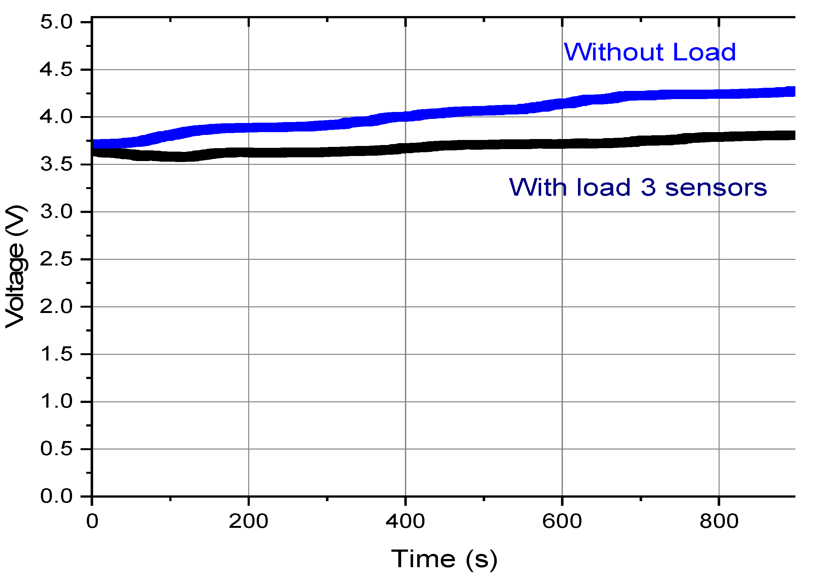
| Vi (V) | Vf (V) | Energy (J) | Power (mW) | |
|---|---|---|---|---|
| Without load | 3.71 | 4.44 | 2.97 | 3.3 |
| With 3 sensors load | 3.71 | 3.85 | 0.52 | 0.6 |
| Frequency f (Hz) | Total Generated Energy E(J) | Total Power PT (mW) | Maximum Number of Sensors N | Energy Used to the Sensors E (J) | Excess Energy Stored ∆E (J) | Excess Power ∆P (mW) |
|---|---|---|---|---|---|---|
| 0.1 | 1.18 | 1.31 | 1 | 0.85 | 0.33 | 0.37 |
| 0.15 | 1.78 | 1.98 | 2 | 1.70 | 0.08 | 0.09 |
| 0.2 | 2.97 | 3.30 | 3 | 2.55 | 0.42 | 0.47 |
| 0.3 | 4.56 | 5.07 | 5 | 4.25 | 0.31 | 0.34 |
| 0.4 | 6.96 | 7.73 | 8 | 6.80 | 0.16 | 0.18 |
Publisher’s Note: MDPI stays neutral with regard to jurisdictional claims in published maps and institutional affiliations. |
© 2022 by the authors. Licensee MDPI, Basel, Switzerland. This article is an open access article distributed under the terms and conditions of the Creative Commons Attribution (CC BY) license (https://creativecommons.org/licenses/by/4.0/).
Share and Cite
Faria, C.L.; Martins, M.S.; Matos, T.; Lima, R.; Miranda, J.M.; Gonçalves, L.M. Underwater Energy Harvesting to Extend Operation Time of Submersible Sensors. Sensors 2022, 22, 1341. https://doi.org/10.3390/s22041341
Faria CL, Martins MS, Matos T, Lima R, Miranda JM, Gonçalves LM. Underwater Energy Harvesting to Extend Operation Time of Submersible Sensors. Sensors. 2022; 22(4):1341. https://doi.org/10.3390/s22041341
Chicago/Turabian StyleFaria, Carlos L., Marcos S. Martins, Tiago Matos, Rui Lima, João M. Miranda, and Luís M. Gonçalves. 2022. "Underwater Energy Harvesting to Extend Operation Time of Submersible Sensors" Sensors 22, no. 4: 1341. https://doi.org/10.3390/s22041341
APA StyleFaria, C. L., Martins, M. S., Matos, T., Lima, R., Miranda, J. M., & Gonçalves, L. M. (2022). Underwater Energy Harvesting to Extend Operation Time of Submersible Sensors. Sensors, 22(4), 1341. https://doi.org/10.3390/s22041341