
High-Frequency Ultrasound Dataset for Deep Learning-Based Image Quality Assessment


Abstract
:1. Introduction
- images distorted by artifacts from trembling hand with the US probe or impurities contained in the ultrasound gel;
- frames captured when the ultrasound probe was not adhered or incorrectly adhered to the patient’s skin, or the angle between the ultrasound probe and the skin was too small (the proper angle is crucial for HFUS image acquisition);
- images with too low contrast for reliable diagnosis, or captured with too little gel volume-improper for epidermis layer detection;
- data with disturbed geometry as well as HFUS frames with common ultrasound artifacts like acoustic enhancement, acoustic shadowing, beam width artifact, etc.
2. Materials
3. Methods
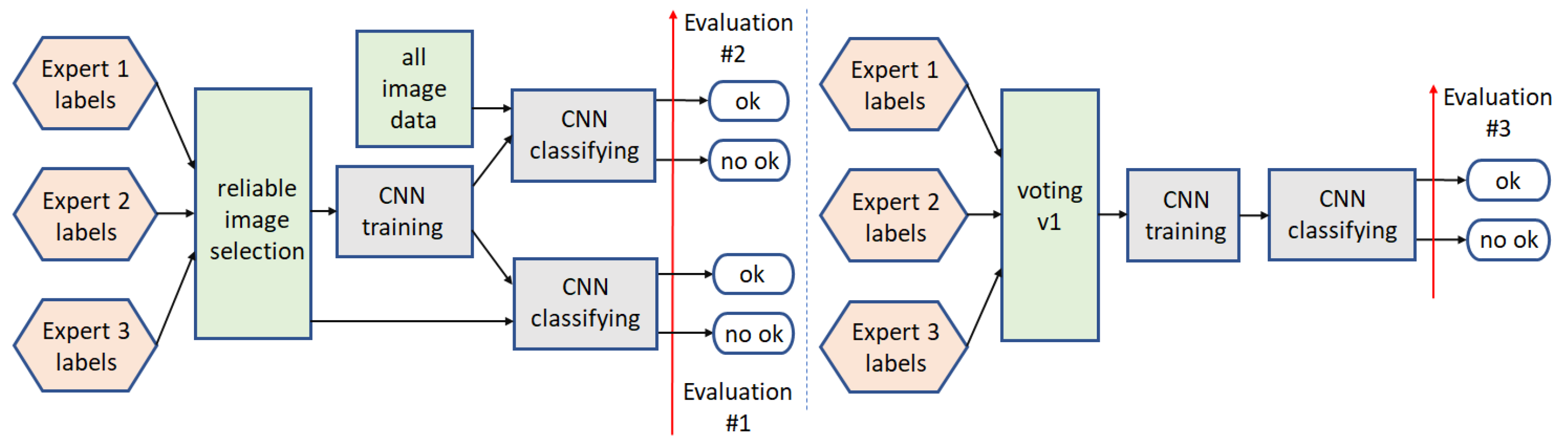
3.1. Binary Classification
3.1.1. Path1
3.1.2. Path2
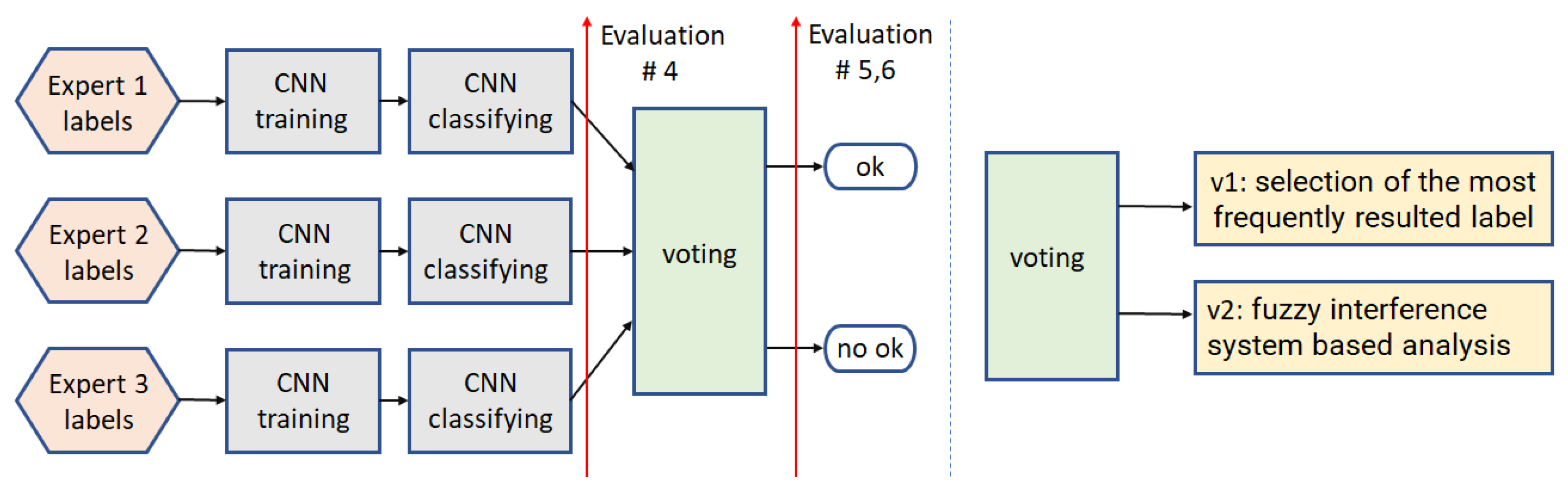
3.1.3. Path3
3.1.4. Path4
3.2. Multi-Class Analysis
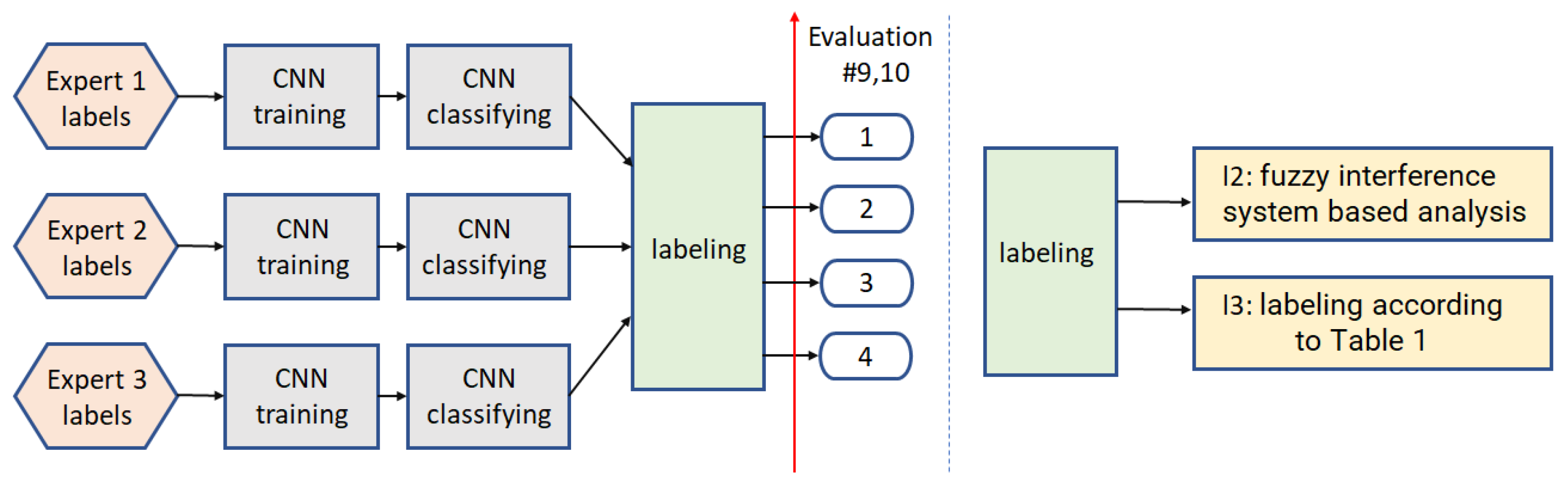
3.2.1. Path5
3.2.2. Path6
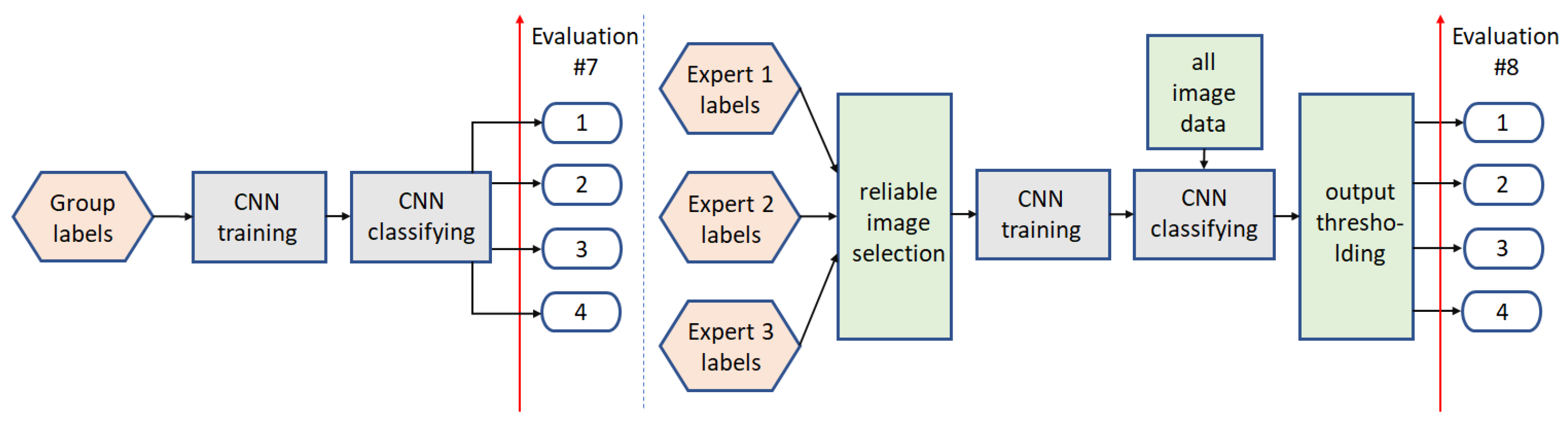
3.2.3. Path7
3.2.4. Path8
4. Experiments and Results
5. Discussion and Conclusions
Author Contributions
Funding
Institutional Review Board Statement
Informed Consent Statement
Data Availability Statement
Conflicts of Interest
References
- Bezugly, A.; Sedova, T.; Belkov, P.; Enikeev, D.; Voloshin, R. Nevus sebaceus of Jadassohn—High frequency ultrasound imaging and videodermoscopy examination. Case presentation. Med. Pharm. Rep. 2020, 94, 112. [Google Scholar] [CrossRef] [PubMed]
- Czajkowska, J.; Badura, P.; Korzekwa, S.; Płatkowska-Szczerek, A. Deep learning approach to skin layers segmentation in inflammatory dermatoses. Ultrasonics 2021, 114, 106412. [Google Scholar] [CrossRef] [PubMed]
- Levy, J.; Barrett, D.L.; Harris, N.; Jeong, J.J.; Yang, X.; Chen, S.C. High-frequency ultrasound in clinical dermatology: A review. Ultrasound J. 2021, 13, 1–12. [Google Scholar] [CrossRef] [PubMed]
- Czajkowska, J.; Badura, P.; Korzekwa, S.; Płatkowska-Szczerek, A.; Słowińska, M. Deep Learning-Based High-Frequency Ultrasound Skin Image Classification with Multicriteria Model Evaluation. Sensors 2021, 21, 5846. [Google Scholar] [CrossRef] [PubMed]
- Bhatta, A.; Keyal, U.; Liu, Y. Application of high frequency ultrasound in dermatology. Discov. Med. 2018, 26, 237–242. [Google Scholar]
- Heibel, H.D.; Hooey, L.; Cockerell, C.J. A Review of Noninvasive Techniques for Skin Cancer Detection in Dermatology. Am. J. Clin. Dermatol. 2020, 21, 513–524. [Google Scholar] [CrossRef] [PubMed]
- Kleinerman, R.; Whang, T.B.; Bard, R.L.; Marmur, E.S. Ultrasound in dermatology: Principles and applications. J. Am. Acad. Dermatol. 2012, 67, 478–487. [Google Scholar] [CrossRef]
- Sciolla, B.; Delachartre, P.; Cowell, L.; Dambry, T.; Guibert, B. Improved boundary segmentation of skin lesions in high-frequency 3D ultrasound. Comput. Biol. Med. 2017, 87, 302–310. [Google Scholar] [CrossRef]
- Hurnakova, J.; Filippucci, E.; Cipolletta, E.; Di Matteo, A.; Salaffi, F.; Carotti, M.; Draghessi, A.; Di Donato, E.; Di Carlo, M.; Lato, V.; et al. Prevalence and distribution of cartilage damage at the metacarpal head level in rheumatoid arthritis and osteoarthritis: An ultrasound study. Rheumatology 2019, 58, 1206–1213. [Google Scholar] [CrossRef] [Green Version]
- Cipolletta, E.; Fiorentino, M.C.; Moccia, S.; Guidotti, I.; Grassi, W.; Filippucci, E.; Frontoni, E. Artificial Intelligence for Ultrasound Informative Image Selection of Metacarpal Head Cartilage. A Pilot Study. Front. Med. 2021, 8, 88. [Google Scholar] [CrossRef]
- Chen, L.; Chen, J.; Hajimirsadeghi, H.; Mori, G. Adapting Grad-CAM for Embedding Networks. In Proceedings of the IEEE/CVF Winter Conference on Applications of Computer Vision (WACV), Snowmass, CO, USA, 1–5 March 2020; pp. 2783–2792. [Google Scholar] [CrossRef]
- Polańska, A.; Silny, W.; Jenerowicz, D.; Knioła, K.; Molińska-Glura, M.; Dańczak-Pazdrowska, A. Monitoring of therapy in atopic dermatitis–observations with the use of high-frequency ultrasonography. Ski. Res. Technol. 2015, 21, 35–40. [Google Scholar] [CrossRef] [PubMed]
- Czajkowska, J.; Korzekwa, S.; Pietka, E. Computer Aided Diagnosis of Atopic Dermatitis. Comput. Med. Imaging Graph. 2020, 79, 101676. [Google Scholar] [CrossRef]
- Marosán, P.; Szalai, K.; Csabai, D.; Csány, G.; Horváth, A.; Gyöngy, M. Automated seeding for ultrasound skin lesion segmentation. Ultrasonics 2021, 110, 106268. [Google Scholar] [CrossRef]
- Sciolla, B.; Digabel, J.L.; Josse, G.; Dambry, T.; Guibert, B.; Delachartre, P. Joint segmentation and characterization of the dermis in 50 MHz ultrasound 2D and 3D images of the skin. Comput. Biol. Med. 2018, 103, 277–286. [Google Scholar] [CrossRef] [PubMed]
- Gao, Y.; Tannenbaum, A.; Chen, H.; Torres, M.; Yoshida, E.; Yang, X.; Wang, Y.; Curran, W.; Liu, T. Automated Skin Segmentation in Ultrasonic Evaluation of Skin Toxicity in Breast Cancer Radiotherapy. Ultrasound Med. Biol. 2013, 39, 2166–2175. [Google Scholar] [CrossRef] [PubMed] [Green Version]
- Czajkowska, J.; Badura, P.; Korzekwa, S.; Płatkowska-Szczerek, A. Automated segmentation of epidermis in high-frequency ultrasound of pathological skin using a cascade of DeepLab v3+ networks and fuzzy connectedness. Comput. Med. Imaging Graph. 2021, 95, 102023. [Google Scholar] [CrossRef]
- Nguyen, K.L.; Delachartre, P.; Berthier, M. Multi-Grid Phase Field Skin Tumor Segmentation in 3D Ultrasound Images. IEEE Trans. Image Process. 2019, 28, 3678–3687. [Google Scholar] [CrossRef]
- Czajkowska, J.; Dziurowicz, W.; Badura, P.; Korzekwa, S. Deep Learning Approach to Subepidermal Low Echogenic Band Segmentation in High Frequency Ultrasound. In Information Technology in Biomedicine; Springer International Publishing: Berlin/Heidelberg, Germany, 2020. [Google Scholar] [CrossRef]
- del Amor, R.; Morales, S.; Colomer, A.; Mogensen, M.; Jensen, M.; Israelsen, N.M.; Bang, O.; Naranjo, V. Automatic Segmentation of Epidermis and Hair Follicles in Optical Coherence Tomography Images of Normal Skin by Convolutional Neural Networks. Front. Med. 2020, 7, 220. [Google Scholar] [CrossRef]
- Huang, Q.; Zhang, F.; Li, X. Machine Learning in Ultrasound Computer-Aided Diagnostic Systems: A Survey. BioMed Res. Int. 2018, 2018, 1–10. [Google Scholar] [CrossRef]
- Cai, L.; Gao, J.; Zhao, D. A review of the application of deep learning in medical image classification and segmentation. Ann. Transl. Med. 2020, 8, 713. [Google Scholar] [CrossRef]
- Liu, S.; Wang, Y.; Yang, X.; Lei, B.; Liu, L.; Li, S.X.; Ni, D.; Wang, T. Deep Learning in Medical Ultrasound Analysis: A Review. Engineering 2019, 5, 261–275. [Google Scholar] [CrossRef]
- Han, S.; Kang, H.K.; Jeong, J.Y.; Park, M.H.; Kim, W.; Bang, W.C.; Seong, Y.K. A deep learning framework for supporting the classification of breast lesions in ultrasound images. Phys. Med. Biol. 2017, 62, 7714–7728. [Google Scholar] [CrossRef] [PubMed]
- Chi, J.; Walia, E.; Babyn, P.; Wang, J.; Groot, G.; Eramian, M. Thyroid Nodule Classification in Ultrasound Images by Fine-Tuning Deep Convolutional Neural Network. J. Digit. Imaging 2017, 30, 477–486. [Google Scholar] [CrossRef]
- Meng, D.; Zhang, L.; Cao, G.; Cao, W.; Zhang, G.; Hu, B. Liver fibrosis classification based on transfer learning and FCNet for ultrasound images. IEEE Access 2017, 5, 5804–5810. [Google Scholar] [CrossRef]
- Burgos-Artizzu, X.P.; Coronado-Gutiérrez, D.; Valenzuela-Alcaraz, B.; Bonet-Carne, E.; Eixarch, E.; Crispi, F.; Gratacós, E. Evaluation of deep convolutional neural networks for automatic classification of common maternal fetal ultrasound planes. Sci. Rep. 2020, 10, 1–12. [Google Scholar] [CrossRef]
- Mendeley Data. Available online: https://data.mendeley.com/ (accessed on 18 January 2022).
- Shared Datasets, Center for Artificial Intelligence in Medicine & Imaging. Available online: https://aimi.stanford.edu/research/public-datasets (accessed on 30 December 2021).
- Czajkowska, J.; Badura, P.; Płatkowska-Szczerek, A.; Korzekwa, S. Data for: Deep Learning Approach to Skin Layers Segmentation in Inflammatory Dermatoses. Available online: https://data.mendeley.com/datasets/5p7fxjt7vs/1 (accessed on 30 December 2021). [CrossRef]
- Karimi, D.; Warfield, S.K.; Gholipour, A. Critical Assessment of Transfer Learning for Medical Image Segmentation with Fully Convolutional Neural Networks. arXiv 2020, arXiv:2006.00356. [Google Scholar]
- van Opbroek, A.; Ikram, M.A.; Vernooij, M.W.; de Bruijne, M. Transfer Learning Improves Supervised Image Segmentation Across Imaging Protocols. IEEE Trans. Med. Imaging 2015, 34, 1018–1030. [Google Scholar] [CrossRef] [PubMed] [Green Version]
- Morid, M.A.; Borjali, A.; Del Fiol, G. A scoping review of transfer learning research on medical image analysis using ImageNet. Comput. Biol. Med. 2021, 128, 104115. [Google Scholar] [CrossRef]
- ImageNet. 2021. Available online: http://www.image-net.org (accessed on 8 April 2021).
- Kim, I.; Rajaraman, S.; Antani, S. Visual Interpretation of Convolutional Neural Network Predictions in Classifying Medical Image Modalities. Diagnostics 2019, 9, 38. [Google Scholar] [CrossRef] [Green Version]
- Kim, J.; Nguyen, A.D.; Lee, S. Deep CNN-Based Blind Image Quality Predictor. IEEE Trans. Neural Netw. Learn. Syst. 2019, 30, 11–24. [Google Scholar] [CrossRef]
- Zhang, S.; Wang, Y.; Jiang, J.; Dong, J.; Yi, W.; Hou, W. CNN-Based Medical Ultrasound Image Quality Assessment. Complexity 2021, 2021, 1–9. [Google Scholar] [CrossRef]
- Wang, X.; Zhang, S.; Liang, X.; Zheng, C.; Zheng, J.; Sun, M. A cnn-based retinal image quality assessment system for teleophthalmology. J. Mech. Med. Biol. 2019, 19, 1950030. [Google Scholar] [CrossRef]
- Gu, K.; Zhai, G.; Yang, X.; Zhang, W. Using Free Energy Principle For Blind Image Quality Assessment. IEEE Trans. Multimed. 2015, 17, 50–63. [Google Scholar] [CrossRef]
- Sun, S.; Yu, T.; Xu, J.; Lin, J.; Zhou, W.; Chen, Z. GraphIQA:Learning Distortion Graph Representations for Blind Image Quality Assessment. arXiv 2021, arXiv:2103.07666v3. [Google Scholar]
- Moorthy, A.K.; Bovik, A.C. Blind Image Quality Assessment: From Natural Scene Statistics to Perceptual Quality. IEEE Trans. Image Process. 2011, 20, 3350–3364. [Google Scholar] [CrossRef] [PubMed]
- Zhou, W.; Chen, Z.; Li, W. Dual-Stream Interactive Networks for No-Reference Stereoscopic Image Quality Assessment. IEEE Trans. Image Process. 2019, 28, 3946–3958. [Google Scholar] [CrossRef]
- Xu, J.; Zhou, W.; Chen, Z. Blind Omnidirectional Image Quality Assessment With Viewport Oriented Graph Convolutional Networks. IEEE Trans. Circuits Syst. Video Technol. 2021, 31, 1724–1737. [Google Scholar] [CrossRef]
- Piccini, D.; Demesmaeker, R.; Heerfordt, J.; Yerly, J.; Sopra, L.D.; Masci, P.G.; Schwitter, J.; Ville, D.V.D.; Richiardi, J.; Kober, T.; et al. Deep Learning to Automate Reference-Free Image Quality Assessment of Whole-Heart MR Images. Radiol. Artif. Intell. 2020, 2, e190123. [Google Scholar] [CrossRef]
- Wu, L.; Cheng, J.Z.; Li, S.; Lei, B.; Wang, T.; Ni, D. FUIQA: Fetal Ultrasound Image Quality Assessment With Deep Convolutional Networks. IEEE Trans. Cybern. 2017, 47, 1336–1349. [Google Scholar] [CrossRef] [PubMed]
- Wang, Z.; Bovik, A.; Sheikh, H.; Simoncelli, E. Image Quality Assessment: From Error Visibility to Structural Similarity. IEEE Trans. Image Process. 2004, 13, 600–612. [Google Scholar] [CrossRef] [Green Version]
- Czajkowska, J.; Juszczyk, J.; Piejko, L.; Glenc-Ambroży, M. High-Frequency Dataset of Facial Skin. Available online: https://doi.org/10.17632/td8r3ty79b.1 (accessed on 10 February 2022).
- Landis, J.R.; Koch, G.G. The measurement of observer agreement for categorical data. Biometrics 1977, 33, 159–174. [Google Scholar] [CrossRef] [PubMed] [Green Version]
- Cardillo, G. Cohen’s Kappa: Compute the Cohen’s Kappa Ratio on a Square Matrix. 2007. Available online: http://www.mathworks.com/matlabcentral/fileexchange/15365 (accessed on 10 February 2022).
- Huang, G.; Liu, Z.; van der Maaten, L.; Weinberger, K.Q. Densely Connected Convolutional Networks. arXiv 2018, arXiv:1608.06993. [Google Scholar]
- Simonyan, K.; Zisserman, A. Very deep convolutional networks for large-scale image recognition. arXiv 2014, arXiv:1409.1556. [Google Scholar]
- Mamdani, E.; Assilian, S. An experiment in linguistic synthesis with a fuzzy logic controller. Int. J. Man-Mach. Stud. 1975, 7, 1–13. [Google Scholar] [CrossRef]


| Group Label | Description | Size |
|---|---|---|
| 1 | all experts labeled the image ‘no ok’ | 8398 |
| 2 | one expert labeled the image ‘no ok’ | 1261 |
| 3 | two experts labeled the image ‘no ok’ | 1324 |
| 4 | all experts labeled the image ‘ok’ | 6442 |
| ID | 8032021 | 15022021 | 12042021 | 7062021 |
|---|---|---|---|---|
| nb. of patients | 43 | 43 | 40 | 40 |
| nb. of images | 4385 | 5840 | 4384 | 2816 |
| ACC | Precision | Recall | f1-Score | ||
|---|---|---|---|---|---|
| Expert1: | DenseNet-201 | 0.8790 | 0.8440 | 0.8723 | 0.8579 |
| VGG16 | 0.8982 | 0.8738 | 0.8849 | 0.8793 | |
| Expert2: | DenseNet-201 | 0.8682 | 0.8322 | 0.8644 | 0.8480 |
| VGG16 | 0.8907 | 0.8713 | 0.8718 | 0.8716 | |
| Expert3: | DenseNet-201 | 0.8802 | 0.8632 | 0.8974 | 0.8800 |
| VGG16 | 0.8999 | 0.8855 | 0.9135 | 0.8993 |
| Kappa | Agreement | Kappa | Agreement | ||
|---|---|---|---|---|---|
| Evaluation#1 | 0.9177 | Perfect | Evaluation#7 | 0.7193 | Substantial |
| Evaluation#2 | 0.8302 | Perfect | Evaluation#8 | 0.6855 | Substantial |
| Evaluation#3 | 0.8214 | Perfect | Evaluation#9 | 0.6808 | Substantial |
| Evaluation#5 | 0.7822 | Substantial | Evaluation#10 | 0.6730 | Substantial |
| Evaluation#6 | 0.8322 | Perfect |
Publisher’s Note: MDPI stays neutral with regard to jurisdictional claims in published maps and institutional affiliations. |
© 2022 by the authors. Licensee MDPI, Basel, Switzerland. This article is an open access article distributed under the terms and conditions of the Creative Commons Attribution (CC BY) license (https://creativecommons.org/licenses/by/4.0/).
Share and Cite
Czajkowska, J.; Juszczyk, J.; Piejko, L.; Glenc-Ambroży, M. High-Frequency Ultrasound Dataset for Deep Learning-Based Image Quality Assessment. Sensors 2022, 22, 1478. https://doi.org/10.3390/s22041478
Czajkowska J, Juszczyk J, Piejko L, Glenc-Ambroży M. High-Frequency Ultrasound Dataset for Deep Learning-Based Image Quality Assessment. Sensors. 2022; 22(4):1478. https://doi.org/10.3390/s22041478
Chicago/Turabian StyleCzajkowska, Joanna, Jan Juszczyk, Laura Piejko, and Małgorzata Glenc-Ambroży. 2022. "High-Frequency Ultrasound Dataset for Deep Learning-Based Image Quality Assessment" Sensors 22, no. 4: 1478. https://doi.org/10.3390/s22041478