Abstract
Sometimes it is difficult, or even impossible, to acquire real data from sensors and machines that must be used in research. Such examples are the modern industrial platforms that frequently are reticent to share data. In such situations, the only option is to work with synthetic data obtained by simulation. Regarding simulated data, a limitation could consist in the fact that the data are not appropriate for research, based on poor quality or limited quantity. In such cases, the design of algorithms that are tested on that data does not give credible results. For avoiding such situations, we consider that mathematically grounded data-quality assessments should be designed according to the specific type of problem that must be solved. In this paper, we approach a multivariate type of prediction whose results finally can be used for binary classification. We propose the use of a mathematically grounded data-quality assessment, which includes, among other things, the analysis of predictive power of independent variables used for prediction. We present the assumptions that should be passed by the synthetic data. Different threshold values are established by a human assessor. In the case of research data, if all the assumptions pass, then we can consider that the data are appropriate for research and can be applied by even using other methods for solving the same type of problem. The applied method finally delivers a classification table on which can be applied any indicators of performed classification quality, such as sensitivity, specificity, accuracy, F1 score, area under curve (AUC), receiver operating characteristics (ROC), true skill statistics (TSS) and Kappa coefficient. These indicators’ values offer the possibility of comparison of the results obtained by applying the considered method with results of any other method applied for solving the same type of problem. For evaluation and validation purposes, we performed an experimental case study on a novel synthetic dataset provided by the well-known UCI data repository.
1. Introduction
The properties of the data (data distribution, etc.), data quality (missing values, outliers, etc.) and quantity are of utmost importance for the efficient functioning of modern data-driven artificial-intelligence applications that are, most of the time, based on machine learning. Based on the available data, we should chose the most appropriate corresponding analyzing methods. Methods that are not chosen based on data property, quality and quantity could lead to the wrong conclusions. This is why it is so important, as a preliminary step, to analyze the data by using appropriate techniques. This is a step that is skipped frequently in research, leading to the application of less appropriate methods, even when more appropriate methods are available.
Often, it is difficult, or even impossible, to obtain real-life data provided by sensors that should be used for evaluation and testing of algorithms/methods. In such a situation, the feasible option is to work with synthetic data obtained by physical systems or the software simulation of real physical systems. Such an illustrative field, in this sense, is the industry, with recent developments related to Industry 4.0 and smart factories. Motivations of the difficulties to obtain real data provided by sensors for research consists of aspects such as confidentiality of data and industry reticence to share data based on considerations such as industrial secrets and industrial competition. Research performed on synthetic data has advantages versus real data, as such research is cheap and can be generated in the necessary quantity and diversity. One of the limitations of synthetic data consists in the fact that we cannot replicate totally real data based on those applied algorithms, as they could give different results than those applied to real data. Based on this respect, we consider that synthetic data should pass data-quality assessments.
In this paper, we present a mathematical modeling for a data-quality assessment for a specific prediction type of problem-solving. The method is called binary logistic regression (BLR), which is alternatively known as bivariate logistic regression, for the evaluation of predictive power of some predictor (independent) variables, which can be by nominal, ordinal or ratio type on a predicted (dependent) dichotomous variable. The result of the prediction admits a binary classification. For the BLR method, we present the assumptions that must be passed preliminarily for the further applicability of the method. We present an interpretation of the results in a case where all the necessary assumptions are passed, being identified the useful predictor variables and their predicting power. The measure of the predictive power, at the same time, is an indicator of the model fit. It is indicated that the predictive power should belong to at least a minimal class of predicting power that must be established by a human assessor (HA) who has an important central role in the data-quality assessment. Appropriate predictive power indicates that further methods can even be applied.
Based on the predicted probability finally is performed a binary classification whose results are retained in a classification table. Based on the values from the classification table, we can apply any indicators of performed classification quality, such as sensitivity, specificity, accuracy, F1 score, area under curve (AUC), receiver operating characteristics (ROCs), true skill statistics (TSS) and Kappa coefficient. These evaluation results offer the possibility of comparison of the results obtained by applying the BLR with results of any other method that can be applied for performing a binary classification based on the same data.
If the required assumptions fail or the prediction power is low, we can analyze the necessity of the introduction of new predictor variables or the exclusion of redundant predictor variables. It can even be that the available data are not appropriate for research purposes.
BLR is mostly known to be applicable in healthcare research. We would like to notice that frequently is not applied correctly by omitting the verification of the necessary assumptions that should pass to be applicable. In this paper, we treat in-depth the subject of correct application and correct interpretation of the results. Based on this fact this paper represents at the same time a guideline for the correct application of BLR in research to avoid misinterpretations of research data.
For evaluation purposes of the data quality assessment, we have performed an experimental evaluation case study using a recently provided synthetic dataset available on the UCI data repository [1]. We have presented and discussed all the performed steps and interpretation of the results.
The upcoming part of the paper is organized as follows: Section 2 presents a survey on the state-of-the-art data quality assessment methods and presented applications of BLR. In Section 3 the assumptions that must be passed by the BLR method are presented, being treated the interpretation of the results. Section 4 presents an experimental data quality assessment evaluation using a synthetic dataset. Finally, the conclusions are formulated.
2. State-of-the-Art Data Quality Assessment
In this section, we present the state-of-the-art regarding the quality assessment of data. Moreover, we present state-of-the-art applications of BLR.
2.1. Mathematical Modeling of Data Quality Assessment
The research-data (this is the case among others of synthetic data) property, as well as some other characterizing information, if available, has a significant influence on the appropriateness of the application of specific algorithms. This sometimes could require specific preliminary data analysis and use of available information, hereafter, requiring data-quality assessment. Just to mention a very simple example, for instance, in the case of a search problem in a set of numbers, any times can be applied to the sequential search algorithm. If it is known that the numbers are ordered (the ordering property can be algorithmically verified), then we can apply the binary search algorithm. If it is available, the additional information that the ordered set of numbers will be frequently updated the application in the following of binary search is not appropriate. The motivation consists in the fact that each operation (modification, deletion and adding) should be performed in such a way that the numbers maintain the ordering property, which gives computational complexity if they are frequently executed.
Recently a large effort has been made regarding the development of explainable artificial intelligence (EAI). Applications of EAI include the forecast of climate-change consequences [2] and learning the mental-health impact of COVID-19 in the United States [3]. Matzka [4] presented research performed regarding explainable artificial intelligence applied for predictive maintenance applications on a specific recent dataset available on the UCI data repository [1]. The principal contribution consisted of the design of an explainable model and an explanatory interface. The applied training was performed by using the UCI dataset [1]. Finally, the explanatory performance was evaluated and used for making comparisons. In our research presented in this paper, we used the same dataset [1].
There are diverse approaches in the scientific literature specialized in the quality assessment of different types of data. Wu et al. [5] studied the subject of deraining quality assessment in evaluating some types of images. Ben-Dor et al. [6] performed a quality assessment for several methods, using synthetic imaging spectroscopy data. Dell’Amore et al. [7] assessed the image quality of synthetic aperture radar. Friedrich et al. [8] studied the subjects of data creation and data-quality assessment for databases that are usually used in airports. Papacharalampopoulos et al. [9] performed a deep quality assessment for a solar reflector that was built on synthetic data. Masoum et. al. [10] performed a data-quality assessment of different saffron samples, employing data by second-order spectrophotometric-type, applying methods based on three-way chemometry. Fernández et al. [11] presented an estimation performed online of the electric arc furnace tap temperature.
Some mathematical modeling strategies of data-quality assessment are based on binary classification. DiFilippo [12] presented an assessment method that can be applied on SPECT and PET phantom images utilizing binary classification. Hoeijmakers [13] proposed an accuracy assessment of thermoacoustic instability models that involved binary classification.
Recent advances in neuroimaging research have begun to focus on the study of the interactions held at the level of brain regions. Garg et al. [14] proposed a causality analysis that is appropriate for fMRI data. The analysis, also called Granger causality, provides an efficient method for modeling the interactions treated at the spatiotemporal level that are held among the brain regions. The mentioned method applies to full-brain fMRI data.
Wang [15] proposes the use of Cohen’s Kappa, which is frequently applied in research as a quality measure for data annotations for binary classification tasks.
Saad et al. [16] performed research on improving the prediction power of the so-called chemometric models. This is realized through the exploitation of the supplied spectrophotometric data. The research also included a comprehensive bibliographic study. They mainly studied the outcome of data manipulation in the initial data-preprocessing step continuing with the application of chemometric models. Finally, the prediction power of the diverse models was matched by using a validation set consisting of eight mixtures. The statistical comparison was performed by using a two-factor Analysis of Variance. For additional comparison of the predictability of different built models, the prediction based on root-mean-squares error was compared.
2.2. State-of-the-Art Applications of Binary Logistic Regression
Applications of logistic regression are diverse, including processing of tomography [17], detection of rice seed purity [18], classification of scenes [19], spectral and spatial-based classification [20], prediction of axillary lymph node metastases [21], active smoking and associated behavioral risk factors before and during pregnancy [22]. BLR belongs to the class of logistic regression.
In the following, we present examples that illustrate the wide diversity of applications of BLR individually or in combination with other methods.
The applications in healthcare basically can be classified into two classes [23,24,25], namely prognostic prediction and diagnostic prediction. Prognostic prediction consists of the estimation of forming a particular disease throughout a specific period. Diagnostic prediction consists of the estimation of the probability of the presence of a considered disease. In the case of healthcare applications, we must also analyze the very important legal aspects. Reference [26] presents a valuable interdisciplinary study of the actual technical and legal challenges of data quality in the context of European medical law.
Saha et al. [27] treated the problem of predicting deforestation at the Gumani River Basin located in India. Cui et al. [28] presented research on driving forces of the urban hot spots. Barnieh et al. [29] studied the causal drivers of vegetation occurrence situated in West Africa. Ozen [30] presented research on damage gravity intensity assessment of pedestrian accidents. Sanchez-Varela et al. [31] presented research on the performing prediction of damage of status by applying procedures called active arranging training. Manoharan et al. [32] treated the problem of smart-grid checking by applying wireless devices. Lopez and Rodriguez [33] treated the problem of forecasting flash floods in Sao Paulo city. Gonzalez-Betancor and Dorta-Gonzalez [34] treated the subject of the danger of disruption of doctoral research and the problem of mental health in doctoral students.
Tesema et al. [35] presented performed research on trends of infant mortality in Ethiopia. The mathematical modeling was based on BLR with mixed-effect combined with analysis based on multivariate decomposition.
Ferencek and Borstnar [36] presented data-quality-assessment models applied for product failure prediction. The authors studied the failure prediction problem during the product warranty period. They proposed a machine-learning method that is able to decrease in time the error of prediction. From the initial 33 attributes, they detected seven with effective predicting power. One of the conclusions of the research was that the number of collected data was small associated with its cost.
Choi et al. [37] studied the problem of improving predictions efficiency by applying a method based on an artificial neural network resulting in a data-quality-assessment procedure. In the framework of a performed case study, the application to local scour across bridge piers was reported. The motivation of the performed research was based on the assumption of the authors that some methods based on artificial intelligence do not predict field-scale local scour with the necessary accuracy. The research included multivariate (methods applied: Euclidean distance and Mahalanobis distance) and univariate methods, and, finally, the obtained results are compared. The paper gives quantitative descriptions about the degree to how much the data-quality assessment improves predictions.
3. The Method Proposed for Data Quality Assessment
Approaches based on statistics are used for many real-life problem-solving situations [38,39,40,41]. Ref. [39] presented research focused on the study of the phytoremediation potential of crop plants. Regression analysis [42] is a statistical technique for estimating the strength of relationships among variables. Regression analysis includes the logistic regression that most frequently is applied in healthcare [43]. For instance, diverse medical scales for assessing the severity of a patient’s illness have been developed by using logistic regression [44,45,46,47].
Research regarding logistic regression involves one or more predictor (independent) variables and one predicted (dependent) variable. The logistic regression where the dependent variable is dichotomous (take two values) is called binary logistic regression (BLR), sometimes called binomial logistic regression. In our study, we consider the application of BLR. The BLR can be used with the purpose to check whether cases can be correctly predicted in two classes denoted as ClassA and ClassB. ClassA signifies the event occurring, for instance, an engine in a smart factory failed. ClassB signifies the event not occurring, for instance, an engine in a smart factory NOT failed. BLR calculates/estimates the probability of a case belonging to the specific ClassA. Let us denote with P the estimated probability of the event occurring. HA must establish a cut value denoted CutV that could take values in the interval [0, 1]. In most cases, the recommended CutV value is 0.5. If p ≥ CutV, the event is classified as occurring, and ClassA is chosen; elsewhere, if p < CutV, the event is classified as not occurring, and ClassB is chosen. BLR can predict whether cases can be accurately predicted/classified from the predictor variables.
Regarding the decision of choosing BLR alternatively with other methods, we must mention the decision that must be followed: When all predictors (can be one or more) are continuous, then a discriminant function analysis can be applied. When all the predictors (can be one or more) are categorical, a logit analysis can be applied. Logistic regression is appropriate even in the case when the predictor variables include both continuous and categorical types.
In the following subsections, we present assumptions that must be verified by using diverse statistical tests to be correctly applicable to the BLR. Moreover, we present the interpretations of the obtained results.
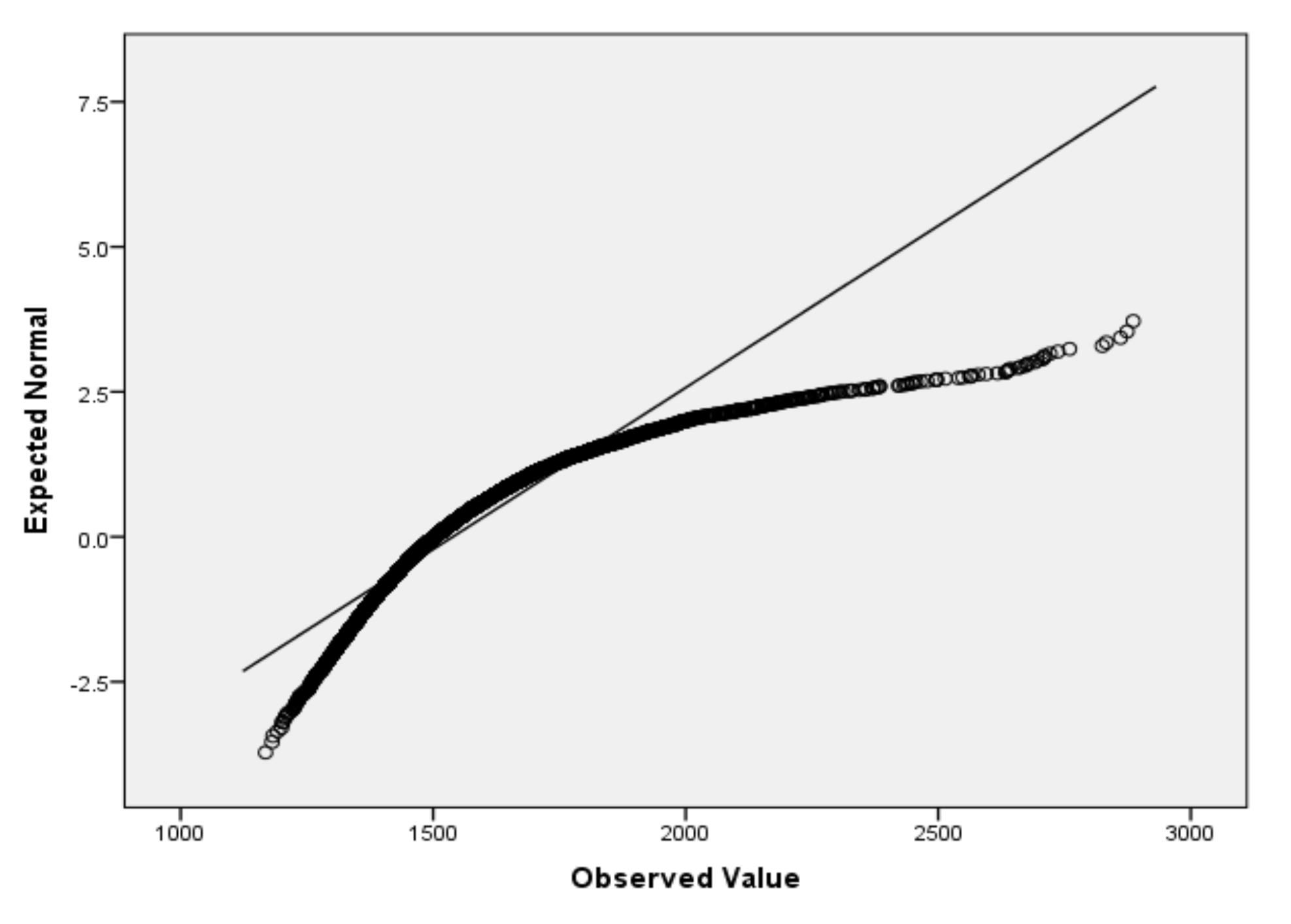
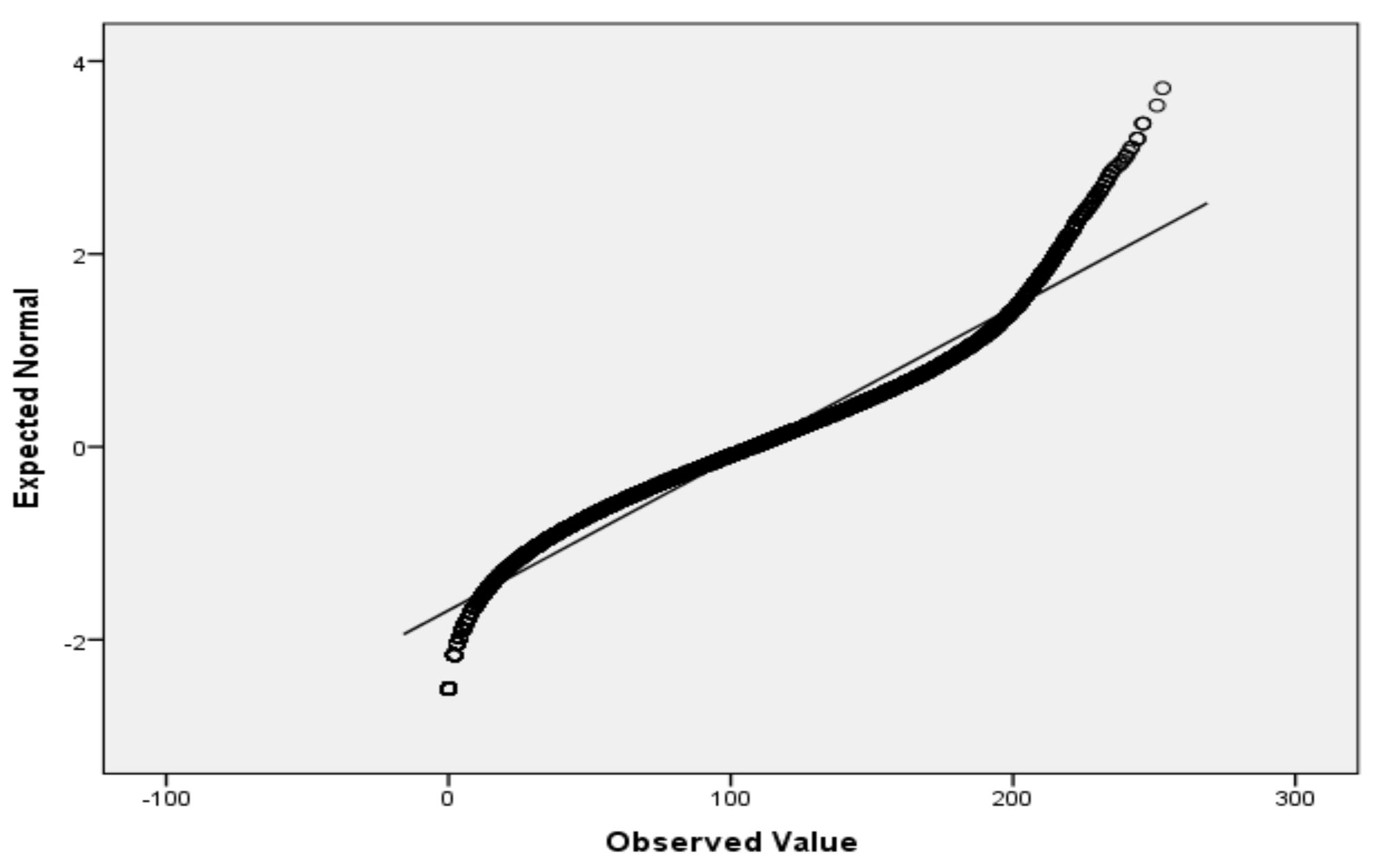
Logistic regression, in contrast to many statistic tests, makes no assumptions about the distributions of the independent variables. If it is useful for interpretation, a verification of normality assumption passing by the independent variables by scale type can be performed. For the verification of the passing of normality assumption for small sample size (3 to 50), we recommend the Shapiro–Wilk test (SW test) [48,49]. SW tests also have the advantage of having the highest statistical power and working well with few data [50]. For a large sample size, we recommend the Lilliefors test [51], which represents an adaptation of Kolmogorov–Smirnov test. Even though both tests can be applied at different significance levels (e.g., 0.01), we recommend the choosing, in most of the cases, the significance level αnorm = 0.05, considering that it is the most appropriate. In the case of both tests, we also recommend the additional visual interpretation of normality by using the Quantile–Quantile plot (QQ plot) scatterplot [52]. In the case of normally distributed data, the points should fall approximately along this reference line. The greater the departure from the reference line, the greater the evidence is for the conclusion that the data fail the normality assumption.
3.1. Basic Assumptions
In this subsection, we present the basic assumptions denoted Basic Assumption 1 (BAss1), Basic Assumption 2 (BAss2), Basic Assumption 3 (BAss3) and Basic Assumption 4 (BAss4), which should pass before the application of BLR.
Basic Assumption 1.
BAss1
The predicted (dependent) variable should be measured on a dichotomous scale. For instance, in the case of a machine or sensor used in the industry, it could indicate the apparition or not of a failure. “C” could indicate correct functioning and “F” could indicate the apparition of failure.
Basic Assumption 2.
BAss2
The predictor (independent) variables (one or more) can take continuous or categorical values. Continuous values can be by interval or ratio type. Categorical values can be ordinal or nominal. The revision time of a machine or a sensor measured in time is an example of a continuous variable.
Ordinal variables can take, for instance, values on the Likert scale [53] by 3 points. For example, the defect of an engine or sensor is by a “small degree” (it can function even in the following), “noticeable” (it must be repaired) or “significant failure” (it is a very grave defect).
As examples of nominal variable values can be mentioned the quality of an engine or sensor that can be “Low” (low quality), “Moderate” (moderate quality), “High” (high quality) or “Excellent” (excellent quality).
In the following, we use the following notations: np denotes the number of predictor variables, and n denotes the total number of cases (data points). In an analysis, the number of valid cases can be smaller than the total number of cases, resulting from the elimination of invalid cases.
Basic Assumption 3.
BAss3
The predicted variable should have categories that are mutually exclusive and exhaustive.
Basic Assumption 4.
BAss4
This assumption states that should be verified for each continuous independent variable the existence of a linear relationship with the logit transformation of the dependent variable. The existence of the linearity can be made, for instance, using the Box–Tidwell method [54].
In the literature, there are proposed also some alternatives to the Box–Tidwell family of transformations to increase its generality. Reference [55] introduces fractional polynomials for Box–Tidwell transformations that have simple rational powers. Reference [56] presents another work on fractional polynomials.
Basic Assumption 5.
BAss5
Sample size estimation for BLR. An important factor for obtaining robust prediction performance is that the size of the dataset should be established relative to the number of predictors [57,58,59,60,61]. In the case of logistic regression, usually, the sample size is established as cases (events) per predictor variable in terms of events per variable (EPV). Low EPV values lead to poor predictive performance [58,60,62,63,64,65]. EPV is defined by the ratio of the number of events. EPV is calculated as the ratio of the number of events relative to the number of predictors.
In medical research, the rule of lower limit by EPV ≥ 10 is frequently used [66]. This criterion has a relatively general acceptance [24,67,68]. Some research [69,70,71] proved that this rule does not perform well in studies that involve large-scale simulation. References [63,65] proved that, when stepwise strategies for choosing predictor variables are applied, the criterion of EPV ≥ 10 is not appropriate. In such situations, it is necessary to apply the EPV ≥ 50 rule [63]. For the estimation of the predictive performance, the paper [72] considers the total sample size, the number of predictors and the events fraction.
3.2. Assumptions That Must Be Passed by the BLR
In this subsection, we present the assumptions, which should be verified by using statistical tests, whose results must pass the threshold values established by HA. If at least one of these assumptions fail, then the application of the BLR is not correct. There are also presented some other statistical tests that must be applied and whose results must be interpreted.
3.2.1. Test for Variables in the Equation Considering the Intercept Only Model
Table 1 presents the study performed for the variables in the equation considering the intercept-only (constant) model. With this purpose is applied Wald’s Chi-Square test. Essential aspects regarding Wald’s test in References [73,74] are presented. In Table 1, we use the following notations: ValWald represents the obtained value of Wald’s test statistics; Valβ represents the value of the obtained β; ValSe represents the value of the standard error; ValSigVE represents the p-value of the Wald’s test; and Exp(β) represents the odds ratio predicted by the model, [Exp(β)] represents the predicted odds of deciding on ClassA, [Exp(β)] = ValExpβ.

Table 1.
Variables in the equation considering the intercept-only model.
In the case of the assumption of Wald’s test, as applied for variables in the equation, it should pass. This means that we must obtain a result for Sigve that is statistically significant. Moreover, αve denotes the significance level of Wald’s test. We recommend that the αve value be 0.05. For the Sigve value, Sigve < αve indicates significance.
Based on Table 1 the intercept-only model can be formulated as (1)
ln(odds) = Valβ,
3.2.2. Omnibus Test of Model Coefficients
When checking the fact that the model is an improvement over the baseline model, we must apply the Omnibus Test of Model Coefficients (OT). It is considered the model with included explanatory variables. OT applies Chi-Square tests for the verification if is a considerable difference between the Log-likelihoods (-2LLs) of the new model and the baseline model. If the model has a significantly increased -2LL comparatively with the baseline, this shows that the new model is explaining more of the variance in the predicted variable, thus indicating the obtainment of an improvement. Moreover, αo denotes the applied significance level of the OT that must be set by HA. The recommended value for αo is 0.01 in most of the cases.
Assumption 1 (Ass1).
Result of Omnibus Test of Model Coefficients.
By applying the OT, we should obtain a statistically significant Chi-Square value. Sigot denotes the obtained p-value of the OT. An Sigot < αo indicates the appropriateness of the application of BLR.
There are three different versions of OT, namely Model, Step and Block. For the comparison of the new model (full model) to the baseline (no model), we should use the version, called Model. The null hypothesis (H0) states that the full model and the baseline model are not statistically significantly different. The rejection of H0 leads to acceptance of alternative hypothesis H1 that allows the formulation of the conclusion that the full model and the baseline model are statistically significantly different. If we apply a stepwise procedure of adding explanatory variables to the model hierarchically, then we should be using the Step and Block.
3.2.3. Hosmer–Lemeshow Test
Hosmer and Lemeshow [75] proposed a goodness-of-fit-test called the Hosmer–Lemeshow (HL) test that is an assumption test for logistic regression models. HL statistic is a reliability indicator of model fit for BLR. This test admits determining whether the model adequately describes the data, and αhl denotes the applied significance level of the HL test that should be set by HA. The recommended value for αhl is 0.05 in most of the situations. Sighl indicates the significance level obtained by applying the HL.
Assumption (Ass2).
Hosmer–Lemeshow test result.
For the BLR to correct applicability, it should verify the criterion of non-significance of the Hosmer–Lemeshow test, Sighl > αhl. The non-significance is an indicator of a good model fit. A significance value, Sighl, lower than 0.05 indicates poor fit and indicates the non-appropriateness of the application of BLR.
3.2.4. The Variance Explained in the Dependent Variable
In this subsection, we address the subject of testing how much variance in the predicted variable can be explained by using the model. More concretely, we present the statistics that can be performed and the interpretation of the results. We also address Assumption 3 (Ass3), which should be verified and passed.
The coefficient of determination in multiple regression analysis is denoted by R2. R2 takes values in the interval [0, 1] and determines the amount of variance in the dependent variable that can be explained by the predictor variables.
In the case of BLR, we should evaluate the pseudo-R2 [76]. As an observation, we would like to mention that the pseudo-R2 values usually have lower values than R2 values in multiple regression. There are different methods proposed in the scientific literature for calculating the pseudo-R2 [76], without having a unanimous agreement on which of them is the most appropriate. In the case of each of them, we can consider advantages and disadvantages. With this purpose, to obtain the explained variance, we can use the likelihood ratio R2 proposed by the Cohen [76], Cox and Snell R2 [77,78], McFadden R2 [78], Tjur R2 [78], and Nagelkerke R2 [76] tests. Tjur R2 is relatively new.
Reference [78] presents a limitation of the Cox and Snell R2. Cox and Snell R2 cannot reach the value 1. The Nagelkerke R2 test provides a correction of the Cox and Snell R2. Among others, the correction includes the elimination of the weakness of not reaching the value 1. The different calculus performed by these two tests provides different results. Reference [78] proposes the use of McFadden R2 instead of Cox and Snell R2. This is based on the different scaling of the tests. In the following, we suggest for interpretation the Nagelkerke R2 value. An obtained NrS value of pseudo-R2 indicates that around NrS% of variance in the dependent variable can be explained by the predictor variables.
Assumption 3 (Ass3).
Minimal variance in the dependent variable that should be explained.
In the case of an experimental evaluation, HA could establish classes of prediction power as follows: “unsatisfactory”, “week”, “appropriate”, “good” and “very good”. Table 2 presents such a proposed classification that could be applied in most of the cases. HA must establish the minimal class to which should be expectable to belong the prediction power of the variables. For instance, HA could establish that it is expectable to belong to at least the class of “good” prediction power.
Table 2.
Prediction power classification established by HA.
Assumption 4 (Ass4).
Measuring how poor is the prediction power.
Additionally, we can calculate the so-called -2 Log-likelihood statistic [79], which represents a measure of how poor the prediction power is. A smaller value of the statistic indicates a better model. The value considered by itself does not provide a clear interpretation. It is useful when more models are compared based on the value of the Log-likelihood. This can be used, for instance, when testing the predicting power of different sets of predictor variables.
3.2.5. Evaluation of Obtained Classification
The results obtained by applying the BLR can be used for making a binary classification. In the following, we consider the assessment of the effectiveness of the predicted classification. It is necessary to assess the effectiveness of the known (correct) classification against the predicted classification. For this, we suggest as a first step the construction of a so-called classification table (CT). Table 3 presents the structure of a CT, consisting of the observed and predicted binary classification. As an example of applicability can be mentioned the machine failure (MF) prediction (a machine fails or not).
Table 3.
Structure of classification table for machine-failure prediction.
In the following is presented the calculus of some indicators that admit the comparison of classification results of BLR with the results of other methods used with the same classification purposes. TN denotes the true negatives: negatives that were correctly classified, TN = Val1. TP denotes the true positives: positives that were correctly classified, TP = Val4. FP denotes the false positives: values that are classified as YES (positives) but are NO (negatives), FP = Val2. FN denotes the false negative: values that are classified as NO (negatives) but are YES (positives), FN = Val3.
Based on the values retained in Table 3, we recommend the calculus of the principal indicators that we consider: sensitivity, specificity and accuracy.
Sensitivity, denoted as ValSENS% in the table, represents the percentage of the cases that had the observed characteristic (“YES” for machine failure); the cases were correctly predicted by the model.
ValSENS% = 100 × (TP/(TP + FN)) = 100 × (Val4/(Val4 + Val3));
Specificity, denoted as ValSPEC% in the table, represents the percentage of cases that did not have the observed characteristic (“NO” for machine failure); these cases were correctly predicted as not having the observed characteristic.
ValSPEC% = 100 × (TN/(TN + FP)) = 100 × (Val1/(Val1 + Val2));
Accuracy represents the percent of correctly predicted positives and negatives. ValTot% from Table 2 denotes the accuracy.
ValTot% = 100 × ((TN + TP)/(TN + TP + FN + FP)) = 100 × ((Val1 + Val4)/(Val1 + Val4 + Val2 + Val3));
Assumption 5 (Ass5).
Classification results evaluation.
Performing the classification and considering the specificity of the research, we should obtain at least a threshold minimal admitted value for one of the following:
- The accuracy indicator;
- All the indicators accuracy, sensitivity and specificity.
This must be established by the human assessor.
Comparing the obtained indicator value(s) with the required one, we can establish the threshold values determined by HA if the classification is in accordance with the expectations. These indicator values admit the comparison with results of other models, based on the fact that HA can choose the most appropriate one. If necessary, HA can choose some other well-known indicators, such as the F1 score [80], AUC [81], ROC [82], TSS [83] and Kappa coefficient [84].
3.2.6. Variables in the Equation with Predictor Variables Included
As a following step, it is applied the Wald Chi-Square test [73,74]. Wald’s test is used for testing the individual contribution of each predictor variable (one or more predictors). Each predictor variable is analyzed in the context of all other predictor variables whose values are kept constant. This procedure has the advantage of being able to eliminate the overlaps between the predictor variables. In the case of a predictor variable, we must verify if it is a statistically significant predictor. It must be applied for each predictor variable at the αSig significance level, which must be set by HA. The significance level, αSig, could take different values, such as 0.05, 0.01 and 0.001. We consider that, in many cases, the most appropriate value is 0.05. In the case of each of the included predictor variables, a value where Sigve < αSig indicates that the variable is a significant predictor. Elsewhere, if in case of a predictor variable, Sigve ≥ αSig indicates that the variable is NOT a significant predictor.
Table 4 presents the variables in the equation with the predictor variables included. The columns in Table 4 have the same labeling as those in Table 1. In Table 1, we use the following notations: β denotes regression weight in the model, SE denotes the standard error, WaldStat denotes the Wald’s test statistics (Wald’s Z value) and EXP(β) denotes the odds ratio (OR). The power of the association between two events can be measured by using the OR.
Table 4.
Variables in the equation with predictor variables included.
For explanatory purposes, we present fictitious data in Table 4 as results regarding the predictor variables in the regression equation. Var1(CatA), Var2 and Var3 denote the predictor variables, where Var1 is a categorical variable, with CatA considered as reference category. Var2 and Var3 take continuous values. The regression coefficients denoted β gives the predicted amount of change in the dependent. Exp(β) is the odds ratio (OR) predicted by the model. OR is calculated by raising the base of the natural Log to the sth power, s denotes the slope that results from the logistic regression equation and CI of EXP(β) denotes the confidence interval of EXP(β) that must be set by HA. It is recommended to choose the 95% confidence level. LowExpβ represents the lower limit of the confidence interval, and UppExpβ represents the upper limit of the confidence interval.
In the following, for illustrative purposes, we interpret the fictitious data from Table 4. Considering Var1, based on the fact that Sigve < αSig (0.01 < 0.05), we can conclude that Var1 is a significant predictor. Considering Var2, based on the fact that Sigve < αSig (0.03 < 0.05), we can conclude that Var2 is a significant predictor. Considering Var3, based on the fact that Sigve > αSig (0.83 > 0.05), we can conclude that Var3 it is NOT a significant predictor.
Exp(β) of Table 4 includes the information for predicting the probability of an event occurring when all other predictor variables are kept constant. For example, in the case of Var1, the table shows that the odds for the “Yes” category are 22.65 times greater for CatA as opposed to CatB.
The Sigve value in the case of each predictor variable gives an answer if the variable is a significant predictor or not. If there are variables that are not significant predictors, this can be reported in the formulated conclusions. If decided, they can be removed, and the analysis can be repeated.
The variables in the equation output obtained for the fictitious data give us the following regression equation, Equation (2):
ln(odds) = −37.7 + 0.78 × Var1 − 0.75 × Var2 + 0.02 × Var3,
The obtained model can be used to predict the odds, based on Equation (3).
Conversion to probabilities should be realized as follows (4):
If decided, we can apply an approach whereby each predictor variable is eliminated step-by-step from the model and is compared to the −2 Log-likelihood statistic of the reduced model with the full model to establish if the reduction is appropriate. Let us consider n to be the number of predictor variables. The previously mentioned approach requires testing of n + 1 models.
3.3. Interpretation of the Binary Logistic Regression Results
An iterative maximum likelihood procedure constructs the model. It starts with values of the regression coefficients generated arbitrarily based on that the construction of an initial model that predicts the observed data. After this, the errors are evaluated and, based on this, the regression coefficients change. This is performed in such a way as to make the observed data likelihood superior for the novel model. This procedure is repeated recursively until the convergence of the model is reached.
In Section 3.1 and Section 3.2, we present all the assumptions that must be passed for the application of BLR to be correct. In this section, we present the interpretation of the obtained results in case of passing all the mandatory assumptions.
In Section 3.2.4, we present the calculus of the pseudo-R2, whose result is denoted NrS. HA considering the specificity of the research must create the interval classes for the value of pseudo-R2 that must be labeled, for instance, in Table 2: “unsatisfactory”, “week”, “appropriate”, “good” and “very good”.
Section 3.2.5 presents the performed classification results in the form of a classification table. Moreover, there are recommended indicators accuracy, sensitivity and specificity. HA considering the specific of the research must establish the thresholds (threshold, minimal acceptance values) for the indicators values that are considered in the interpretation of the results.
4. Experimental Data-Quality-Assessment Evaluation
4.1. The Synthetic Dataset Used in the Evaluation
UCI is a valuable repository of datasets that can be used for research purposes [85]. Reference [1] provides a synthetic dataset created with the intent to mimic real industrial predictive maintenance data. In this section, we briefly present the description of the UCI dataset that we used in the experimental data-quality-assessment evaluation. Reference [4] presents the dataset’s details. Table 5 presents a snapshot of the data with included three cases (numbered with 1, 2 and 78). The whole dataset includes 10,000 rows (cases) of data characterized by six features/variables, organized on separate columns in the table, in the case of real-life data provided by different sensors (e.g., intelligent sensor camera, thermistors, etc.). The features, independent (predictor) variables, are as follows: V1, the product ID; V2, the air temperature (K); V3, the process temperature (K); V4, the rotational speed (rpm); V5, the torque (Nm); and V6, the tool wear (min). Where K denotes the Kelvin temperature scale where zero reflects the complete absence of thermal energy, rpm denotes rotations per minute; Nm denotes the Newton-meter that is a unit of torque in the SI system and min denotes the minutes.
Table 5.
Snapshot of the data used in the research.
V1 values are labeled with the letters “L”, “M” and “H” based on the quality of the product. “L” denotes low-quality products, which consist of 50% of all products. “M” denotes medium quality products, which consist of 30% of all products. “H” denotes high-quality products, which consist of 20% of all products.
Karl Pearson first defined the term “random walk” [86]. Data retained in V2 were generated by utilizing a random-walk process that is later normalized to a standard deviation of 2K around 300K. Data retained in V3 were generated by utilizing a random-walk process that was normalized to a standard deviation of 1K, added to the air temperature plus 10K. Data retained in V4 were calculated from a power of 2860 W, which was overlaid with noise that was normally distributed. Data retained in V5 consisted of the torque values that are normally distributed around 40 Nm with a standard distribution of σ = 10 Nm (note that there are no negative values). Data retained in V6 represent the quality variants H/M/L add 5/3/2 minutes of tool wear to the used tool in the process.
The dependent variable VF is labeled “machine failure”. The retained values indicate whether the machine has failed in a different particular data point. The value 0 indicates no failure. The value 1 indicates the apparition of a failure.
4.2. Experimental Evaluation Results
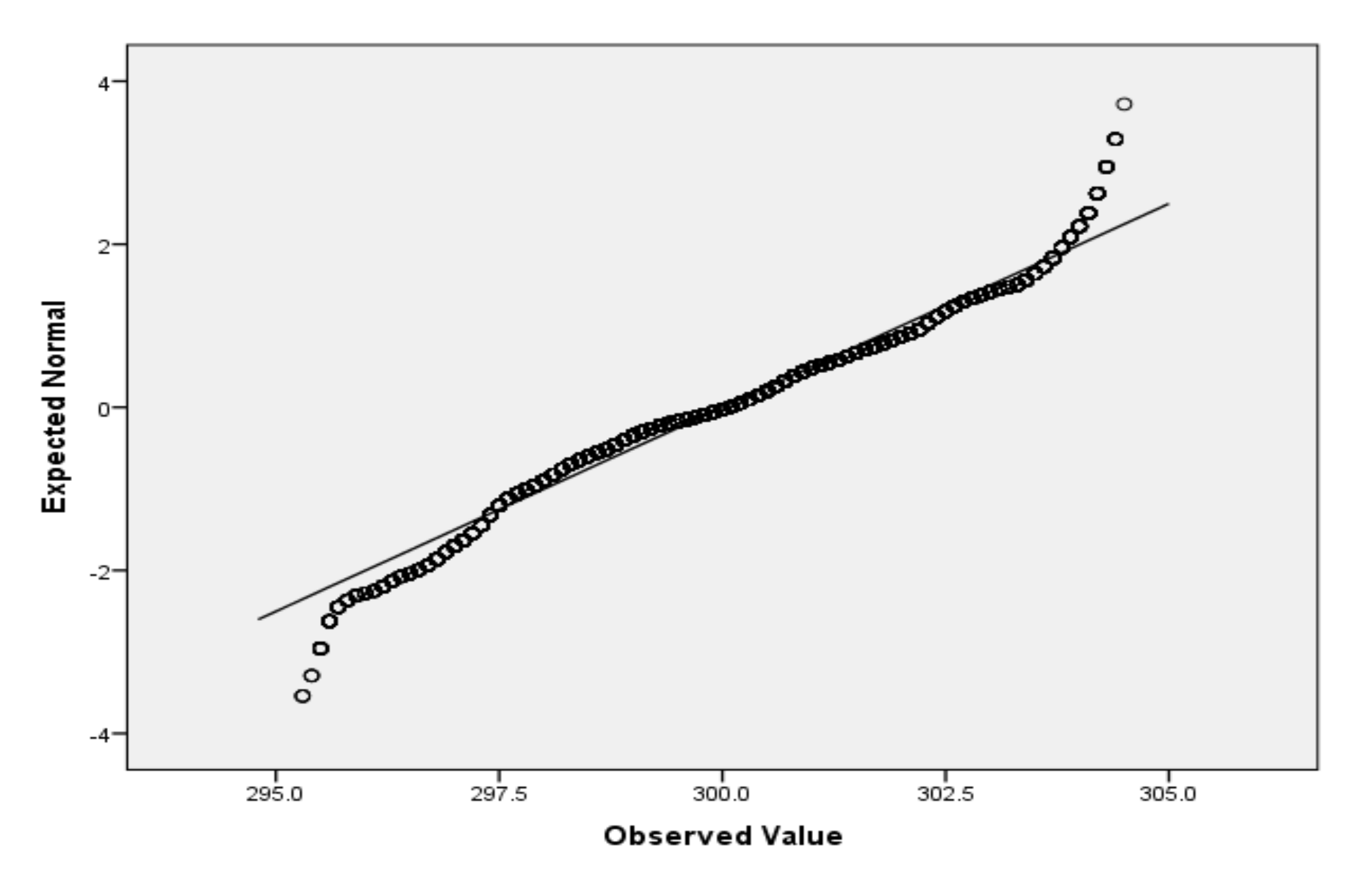
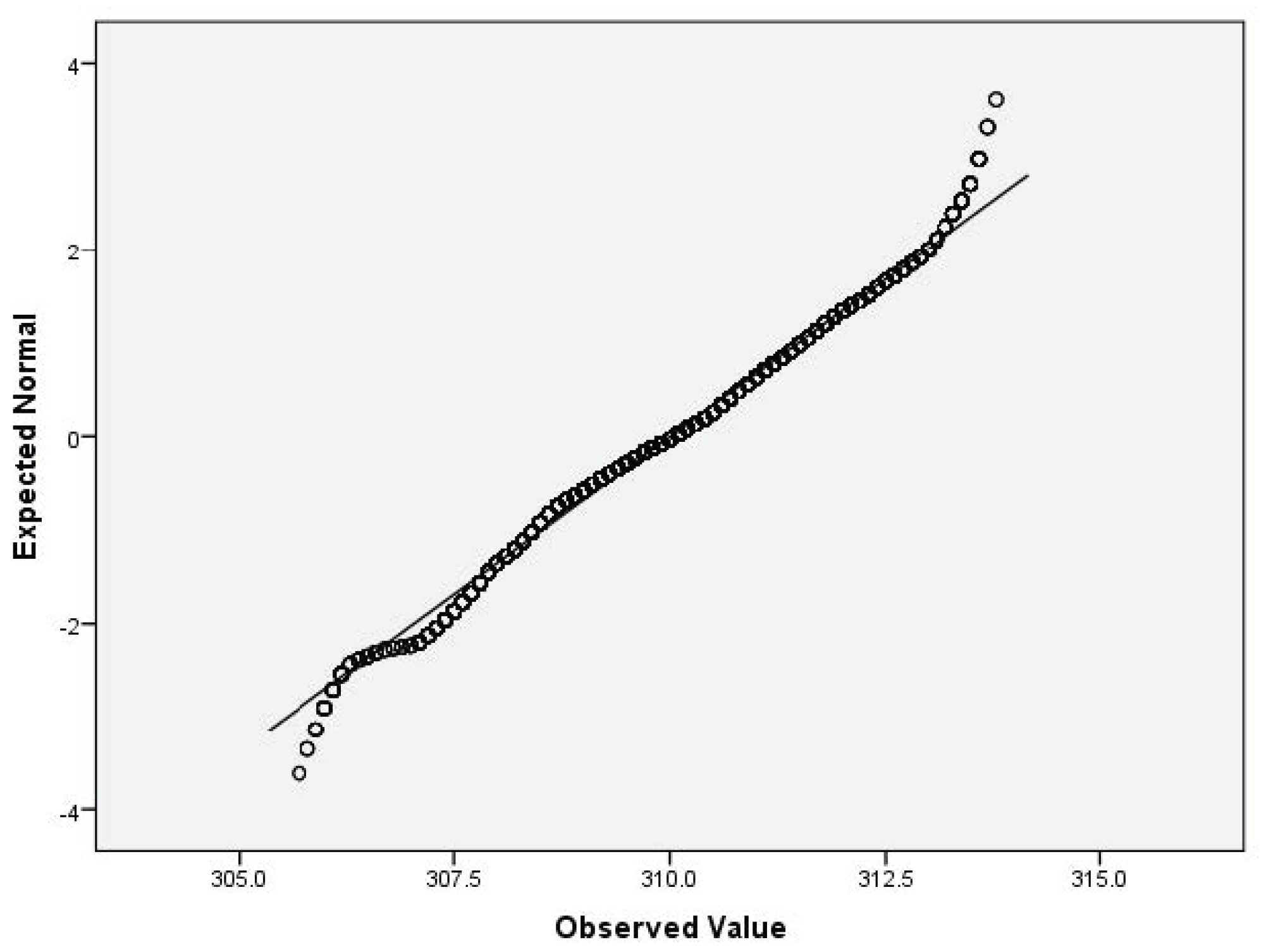
For the variables V2 (air temperature), V3 (process temperature), V4 (rotational speed), V5 (torque) and V6 (tool wear), based on the large sample size, we applied the Lill test with the significance level αnorm = 0.05 (Table 6) and created the QQ plots (Figure 1, Figure 2, Figure 3, Figure 4 and Figure 5) for visual interpretation. The degrees of freedom of each variable is 10,000.
Table 6.
Results of the data normality verification.

Figure 1.
QQ plot for V2.
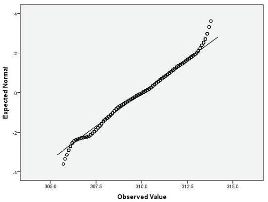
Figure 2.
QQ plot for V3.

Figure 3.
QQ plot for V4.
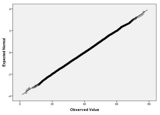
Figure 4.
QQ plot for V5.

Figure 5.
QQ plot for V6.
We performed a BLR on the data presented in Section 4.1. All the cases, 100%, were included in the study, since they were valid (do not contains missing data and outliers). In the experimental evaluation study, we used the following predictor variables: V2 (air temperature), V3 (process temperature), V4 (rotational speed), V5 (torque) and V6 (tool wear).
For the interpretation of the results, we must mention that, in the following, the predicted probability is for the membership for 1 that denotes failure.
- Step 1. Verification of passing all the basic assumptions.
All the basic assumptions, BAss1, BAss2, BAss3, BAss4 and BAss5, received verification that they passed the HA.
- Step 2. Performing the test for the variables in the equation considering the intercept-only model.
Table 7 presents the Wald test results regarding the variables in the equation considering the intercept-only model. The significance level, αve, was set to the value 0.05 by HA. The predicted odds of deciding to continue the research are odds [Exp(B)] = 0.035, which is relatively low. However, the criterion of the significance of variables in the equation passed, Sigve ~ 0, Sigve < αve, indicating a significant result.
Table 7.
Variables in the equation considering the intercept-only model.
- Step 3. Performing the Omnibus Test of Model Coefficients
In the following, we applied the Omnibus Test of Model Coefficients. The value of significance level αot was set to 0.01 by HA. Table 8 presents the results of the OT. According to the previous explanations, it should be interpreted just the line labeled “Model” with the Chi-Square value 1038.064 and Sigot = ~0. The obtained result, Sigot, where Sigot < αot, indicates significant result. However, Assumption Ass1 passed.
Table 8.
Result of the Omnibus Test of Model Coefficients.
- Step 4. Performing the Hosmer–Lemeshow Test
We performed the Hosmer–Lemeshow test. The significance level of the HL, the αhl value, was set to 0.05 by HA. Table 9 presents the results of the HL. Since the p-value of the HL is Sighl > αhl, we can conclude that the criterion of non-significance of HL is satisfied, as is the requirement for the correct application of BLR. Henceforth, we show the good fit of the model. However, assumption Ass2 passed.
Table 9.
Result of the Hosmer–Lemeshow test.
- Step 5: The variance explained in the dependent variable
Regarding the value of pseudo-R2 based on the specific of the research, HA makes the classification that was presented in Table 1. At this step, we calculated the pseudo-R2 by using two methods. Table 10 presents the obtained results of the Cox and Snell R2 and Nagelkerke R2 values. Cox and Snell R2 = 0.099, and Nagelkerke R2 = 0.385.
Table 10.
Obtained pseudo-R2 values.
For the interpretation, we used the Nagelkerke R2 = 0.385 based on motivations previously explained. This obtained value indicates that almost 39% of the variance in the predicted variable can be explained by the predictor variables V2, V3, V4, V5 and V6. The classification results presented in Table 10 indicate a prediction power, which is classified as “good” according to Table 1, 39% ∈ (30%, 40%). However, Ass3 passed. The value of −2 Log-likelihood, Ass4, can be used with comparative purposes to decide which of predictor variables should be maintain, considering their predictive power.
- Step 6. Performing the classification by using the binary logistic regression.
HA established that the classification accuracy must belong to the interval (95%, 100%). Table 11 presents the results of classification obtained by applying BLR.
Table 11.
Performed classification results, with the cut value set to 0.5.
The results presented in Table 11 indicate the classification accuracy by 97%, 97%∈[95%, 100%], which, based on the threshold established by HA, fits the expectation. However, Ass5 passed. It should be mentioned that, in the classification, we used the cut value 0.5. The value of the additionally calculated specificity is ValSPEC% = 99.7%. The value of the additional calculated sensitivity is ValSENS% = 20.1%.
- Step 7. Performing the Wald’s test for the variables in equation with the predictor variables included.
We performed the Wald’s test for the variables in the equation. Table 12 presents the results of Wald’s test, as performed on the variables V2 (air temperature), V3 (process temperature), V4 (rotational speed), V5 (torque) and V6 (tool wear). HA establishes the significance level as αSig = 0.05.
Table 12.
Variables in the equation with the predictor variables included.
For each of the predictor variables, namely V2, V3, V4, V5 and V6, the Wald’s test result Sigve < αSig indicates that the variable is a significant predictor. It is considered the confidence interval, [LowExpβ, UppExpβ] of EXP(β) at the CI = 95% confidence level.
Moreover, we must note the following:
For V2, Exp(β ) > 1 and LowExpβ > 1, UppExpβ > 1.
For V3, Exp(β) < 1 and LowExpβ < 1, UppExpβ < 1.
For V4, Exp(β) > 1 and LowExpβ > 1, UppExpβ > 1.
For V5, Exp(β) > 1 and LowExpβ > 1, UppExpβ > 1.
For V6, Exp(β) > 1 and LowExpβ > 1, UppExpβ > 1.
The regression equation can be formulated based on the results presented in Table 11 as follows (5):
ln(odds)= −36.69 + 0.772 × V2 − 0.743 × V3 + 0.012 × V4 + 0.281 × V5 + 0.013 × V6,
The obtained model can be used to predict the odds, based on Equation (6).
Conversion to probabilities should be realized as follows (7):
- Step 8. Improving the classification by adjusting the cut value.
Regarding the classification choosing the cut value 0.4, the obtained results are presented in Table 13. The accuracy is 97.1% (97% for the cut value 0.5). The value of specificity is ValSPEC% = 99.5% (99.7%, for cut the value 0.5). The value of sensitivity is ValSENS% = 28.3% (20.1% for the cut value 0.5). The obtained results for the cut value 0.4 are better than those obtained for the cut value 0.5.
Table 13.
Performed classification results from using the method with the cut value 0.4.
5. Discussion
Initially, we included in the model the predictor variable V1, along with V2, V3, V4, V5 and V6. The −2 Log-likelihood obtained was 1913.929. Wald’s test for the variables in the equation with Sig = 0.69 indicated the fact that V1 is not a significant predictor. Based on this fact, V1 was removed from the second experimental setup presented in Section 4.2. When verifying the results of the classification table, we observed that we obtained better results with V1 removed. The necessity of a new model was motivated also by the result of the HL test that indicated non-significance.
Briefly, the obtained results presented in the previous section can be interpreted as follows. For the studied synthetic data-quality assessment [1], we applied a BLR. In the case of BLR, we verified the passing of all the necessary assumptions for its applicability. The obtained results indicate the fact that the synthetic data passed the data-quality assessment, indicating that the predicting power is enough to be applicable to binary prediction/classification algorithms. Finally, we presented the classification results based on the applied model, with the cut value 0.4 presented in the form of a classification table, which admits the clear comparison of the results with the prospective results of other methods that can be applied. Based on the value from the classification table, we calculated the accuracy, sensitivity and specificity, but we can use any other indicators, if necessary, such as the F1 score [80], ROC [82], area under the ROC curve (AUC) [81], TSS [83] and Kappa coefficient [84].
The errors that could appear at a classification are the false positives and false negatives. It must be noticed that, in the classification tests, ROC and AUC present how an adjustable threshold causes changes in two types of errors. However, the ROC curve and AUC are only partially meaningful when used with unbalanced data. To avoid this problem, Reference [87] introduced a new concordant partial AUC and a new partial c statistic for ROC.
Regarding the interpretation of the research results, we can say that a BLR was performed to ascertain the effects of V2 (air temperature), V3 (process temperature), V4 (rotational speed), V5 (torque) and V6 (tool wear) on the likelihood of the machine failure. All the assumptions necessary for the application of BLR passed. The applied model explained 38.5% (chosen the Nagelkerke pseudo-R2) of the variance in machine failure. The model correctly classified 97.1% of the cases (with the chosen cut 0.4). Increasing V2 was associated with an increased likelihood of machine failure. Similarly, increasing V4, V5 and V6 were associated with an increased likelihood of machine failure, but the likelihood of failure is smaller than for V2. On the other hand, increasing V3 was associated with a reduction in the likelihood of exhibiting machine failure.
6. Conclusions
In Industry 4.0 and smart factories, there are many challenging binary prediction and classification types of problems that should be solved. Frequently obtaining real industrial data is difficult or even impossible. Based on this fact, very often we should use synthetic data obtained as a result of real or software simulations. In the case of such data, a fundamental subject that should be treated is making a data-quality assessment. We consider that one of the most important aspects of data-quality assessment that should be evaluated is the predictive power. The passing of the data of all the indicated assumptions is an indication for researchers that, on the data, can be applied even other algorithms for binary prediction (classification), offering, at the same time, a comparison measure that is possible to be passed by other algorithms.
The data-quality-assessment fundament was the first objective of the research. For this data-quality-assessment verification, we indicated that a BLR should be performed. By applying this method is obtained the response to the model fits the data. On the obtained classification table, which practically consists of the confusion matrix, we applied the indicators accuracy, sensitivity and specificity. Some others are also recommended to be used when considered appropriate.
BLR is frequently applied in research for solving a binary classification problem and the prediction of the membership to a specific class with a certain probability. Its applicability is best known in medical research. In the case of its application, frequent mistakes result from the fact that the assumptions that should pass to correct its application are not verified. Such mistakes could lead to formulating erroneous conclusions of the research. The second objective of the paper was in making the mathematical grounding of the assumptions that should be verified at the application of the binary logistic regression. These assumptions make it possible for the researchers to apply BLR correctly and correctly interpret the obtained results.
Author Contributions
Conceptualization, L.B.I.; methodology, L.B.I. and C.E.; software, L.B.I.; validation, formal analysis, investigation, L.B.I. and C.E.; resources, L.B.I. and C.E.; data curation, writing—original draft preparation, writing—review and editing, L.B.I. and C.E.; visualization, supervision, C.E. and L.B.I.; project administration, L.B.I.; funding acquisition, C.E. All authors have read and agreed to the published version of the manuscript.
Funding
George Emil Palade University of Medicine, Pharmacy, Science and Technology of Targu Mures.
Institutional Review Board Statement
Not applicable.
Informed Consent Statement
Not applicable.
Data Availability Statement
We used publicly available data for research on UCI data repository [2].
Acknowledgments
This work was developed in the framework of the CHIST-ERA program supported by the Future and Emerging Technologies (FET) program of the European Union through the ERA-NET Cofund funding scheme under the grant agreements of Social Network of Machines (SOON). This research was supported by a grant of the Romanian National Authority for Scientific Research and Innovation, CCCDI-UEFISCDI, project number 101/2019, COFUND-CHISTERA-SOON, within PNCDI III. We would like also to thank you for the Research Center on Artificial Intelligence, Data Science and Smart Engineering (Artemis).
Conflicts of Interest
The authors declare no conflict of interest.
References
- Matzka, S. AI4I 2020 Predictive Maintenance Dataset. UCI Machine Learning Repository. 2020. Available online: www.explorate.ai/dataset/predictiveMaintenanceDataset.csv (accessed on 22 December 2021).
- Chakraborty, D.; Alam, A.; Chaudhuri, S.; Basagaoglu, H.; Sulbaran, T.; Langar, S. Scenario-based prediction of climate change impacts on building cooling energy consumption with explainable artificial intelligence. Appl. Energy 2021, 291, 116807. [Google Scholar] [CrossRef]
- Jha, I.P.; Awasthi, R.; Kumar, A.; Kumar, V.; Sethi, T. Learning the Mental Health Impact of COVID-19 in the United States with Explainable Artificial Intelligence: Observational Study. JMIR Ment. Health 2021, 8, e25097. [Google Scholar] [CrossRef]
- Matzka, S. Explainable Artificial Intelligence for Predictive Maintenance Applications. In Proceedings of the 2020 Third International Conference on Artificial Intelligence for Industries (AI4I), Irvine, CA, USA, 21–23 September 2020; pp. 69–74. [Google Scholar] [CrossRef]
- Wu, Q.B.; Wang, L.; Ngan, K.N.; Li, H.L.; Meng, F.M. Beyond Synthetic Data: A Blind Deraining Quality Assessment Metric Towards Authentic Rain Image. In Proceedings of the 26th IEEE International Conference on Image Processing (ICIP), Taipei, Taiwan, 22–25 September 2019; pp. 2364–2368. [Google Scholar]
- Ben-Dor, E.; Kindel, B.; Goetz, A.F.H. Quality assessment of several methods to recover surface reflectance using synthetic imaging spectroscopy data. Remote Sens. Environ. 2004, 90, 389–404. [Google Scholar] [CrossRef]
- Dell’Amore, L.; Villano, M.; Krieger, G. Assessment of Image Quality of Waveform-Encoded Synthetic Aperture Radar Using Real Satellite Data. In Proceedings of the 20th International Radar Symposium (IRS), Ulm, Germany, 26–28 June 2019. [Google Scholar]
- Friedrich, A.; Raabe, H.; Schiefele, J.; Dorr, K.U. Airport-databases for 3D synthetic-vision flight-guidance displays database design, quality-assessment and data generation, Conference on Enhanced and Synthetic Vision 1999. Proc. SPIE 1999, 3691, 108–115. [Google Scholar]
- Papacharalampopoulos, A.; Tzimanis, K.; Sabatakakis, K.; Stavropoulos, P. Deep Quality Assessment of a Solar Reflector Based on Synthetic Data: Detecting Surficial Defects from Manufacturing and Use Phase. Sensors 2020, 20, 5481. [Google Scholar] [CrossRef]
- Masoum, S.; Gholami, A.; Hemmesi, M.; Abbasi, S. Quality assessment of the saffron samples using second-order spectrophotometric data assisted by three-way chemometric methods via quantitative analysis of synthetic colorants in adulterated saffron. Spectrochim. Acta Part A Mol. Biomol. Spectrosc. 2015, 148, 389–395. [Google Scholar] [CrossRef] [PubMed]
- Fernández, J.M.M.; Cabal, V.A.; Montequin, V.R.; Balsera, J.V. Online estimation of electric arc furnace tap temperature by using fuzzy neural networks. Eng. Appl. Artif. Intell. 2008, 21, 1001–1012. [Google Scholar] [CrossRef]
- DiFilippo, F.P. Assessment of PET and SPECT phantom image quality through automated binary classification of cold rod arrays. Med. Phys. 2019, 46, 3451–3461. [Google Scholar] [CrossRef]
- Hoeijmakers, M.; Arteaga, I.L.; Kornilov, V.; Nijmeijer, H.; de Goey, P. Accuracy assessment of thermoacoustic instability models using binary classification. Int. J. Spray Combust. Dyn. 2013, 5, 201–223. [Google Scholar] [CrossRef] [Green Version]
- Garg, R.; Cecchi, G.A.; Rao, A.R. Causality Analysis of fMRI Data, Conference on Medical Imaging 2011—Biomedical Applications in Molecular, Structural, and Functional Imaging. Proc. SPIE 2011, 7965, 796502. [Google Scholar]
- Wang, J.; Yang, Y.Y.; Xia, B. A Simplified Cohen’S Kappa for Use in Binary Classification Data Annotation Tasks. IEEE Access 2019, 7, 164386–164397. [Google Scholar] [CrossRef]
- Saad, A.S.; Hamdy, A.M.; Salama, F.M.; Abdelkawy, M. Enhancing prediction power of chemometric models through manipulation of the fed spectrophotometric data: A comparative study. Spectrochim. Acta Part A Mol. Biomol. Spectrosc. 2016, 167, 12–18. [Google Scholar] [CrossRef] [PubMed]
- Rymarczyk, T.; Kozlowski, E.; Klosowski, G.; Niderla, K. Logistic Regression for Machine Learning in Process Tomography. Sensors 2019, 19, 3400. [Google Scholar] [CrossRef] [PubMed] [Green Version]
- Liu, W.H.; Zeng, S.; Wu, G.J.; Li, H.; Chen, F.F. Rice Seed Purity Identification Technology Using Hyperspectral Image with LASSO Logistic Regression Model. Sensors 2021, 21, 4384. [Google Scholar] [CrossRef] [PubMed]
- Ahmed, A.; Jalal, A.; Kim, K. A Novel Statistical Method for Scene Classification Based on Multi-Object Categorization and Logistic Regression. Sensors 2020, 20, 3871. [Google Scholar] [CrossRef]
- Mallinis, G.; Koutsias, N. Spectral and Spatial-Based Classification for Broad-Scale Land Cover Mapping Based on Logistic Regression. Sensors 2008, 8, 8067–8085. [Google Scholar] [CrossRef] [Green Version]
- Xie, F.; Yang, H.P.; Wang, S.; Zhou, B.; Tong, F.Z.; Yang, D.Q.; Zhang, J.Q. A Logistic Regression Model for Predicting Axillary Lymph Node Metastases in Early Breast Carcinoma Patients. Sensors 2012, 12, 9936–9950. [Google Scholar] [CrossRef] [Green Version]
- Ruta, F.; Avram, C.; Voidazan, S.; Marginean, C.; Bacarea, V.; Abram, Z.; Foley, K.; Fogarasi-Grenczer, A.; Penzes, M.; Tarcea, M. Active Smoking and Associated Behavioural Risk Factors before and during Pregnancy—Prevalence and Attitudes among Newborns’ Mothers in Mures County, Romania. Cent. Eur. J. Public Health 2016, 24, 276–280. [Google Scholar] [CrossRef]
- Bouwmeester, W.; Zuithoff, N.P.; Mallett, S.; Geerlings, M.I.; Vergouwe, Y.; Steyerberg, E.W.; Altman, D.G.; Moons, K.G. Reporting and methods in clinical prediction research: A systematic review. PLoS Med. 2012, 9, e1001221. [Google Scholar] [CrossRef] [Green Version]
- Moons, K.G.; Altman, D.G.; Reitsma, J.B.; Ioannidis, J.P.; Macaskill, P.; Steyerberg, E.W.; Vickers, A.J.; Ransohoff, D.F.; Collins, G.S. Transparent reporting of a multivariable prediction model for individual prognosis or diagnosis (TRIPOD): Explanation and elaboration. Ann. Intern. Med. 2015, 162, W1–W73. [Google Scholar] [CrossRef] [Green Version]
- Collins, G.S.; Reitsma, J.B.; Altman, D.G.; Moons, K.G. Transparent reporting of a multivariable prediction model for individual prognosis or diagnosis (TRIPOD): The TRIPOD statement. Ann. Intern. Med. 2015, 162, 55. [Google Scholar] [CrossRef] [PubMed] [Green Version]
- Stöger, K.; Schneeberger, D.; Kieseberg, P.; Holzinger, A. Legal aspects of data cleansing in medical AI. Comput. Law Secur. Rev. 2021, 42, 105587. [Google Scholar] [CrossRef]
- Saha, S.; Saha, M.; Mukherjee, K.; Arabameri, A.; Ngo, P.T.T.; Paul, G.C. Predicting the deforestation probability using the binary logistic regression, random forest, ensemble rotational forest, REPTree: A case study at the Gumani River Basin, India. Sci. Total Environ. 2020, 730, 139197. [Google Scholar] [CrossRef] [PubMed]
- Cui, H.F.; Wu, L.; Hu, S.; Lu, R.J.; Wang, S.L. Research on the driving forces of urban hot spots based on exploratory analysis and binary logistic regression model. Trans. GIS 2021, 25, 1522–1541. [Google Scholar]
- Barnieh, B.A.; Jia, L.; Menenti, M.; Jiang, M.; Zhou, J.; Zeng, Y.L.; Bennour, A. Modeling the Underlying Drivers of Natural Vegetation Occurrence in West Africa with Binary Logistic Regression Method. Sustainability 2021, 13, 4673. [Google Scholar] [CrossRef]
- Ozen, M. Injury Severity Level Examination of Pedestrian Crashes: An Application of Binary Logistic Regression. Teknik Dergi 2021, 32, 10859–10883. [Google Scholar]
- Sanchez-Varela, Z.; Boullosa-Falces, D.; Barrena, J.L.L.; Gomez-Solaeche, M.A. Prediction of Loss of Position during Dynamic Positioning Drilling Operations Using Binary Logistic Regression Modeling. J. Mar. Sci. Eng. 2021, 9, 139. [Google Scholar] [CrossRef]
- Manoharan, H.; Teekaraman, Y.; Kirpichnikova, I.; Kuppusamy, R.; Nikolovski, S.; Baghaee, H.R. Smart Grid Monitoring by Wireless Sensors Using Binary Logistic Regression. Energies 2020, 13, 3974. [Google Scholar] [CrossRef]
- Lopez, A.S.V.; Rodriguez, C.A.M. Flash Flood Forecasting in Sao Paulo Using a Binary Logistic Regression Model. Atmosphere 2020, 11, 473. [Google Scholar] [CrossRef]
- Gonzalez-Betancor, S.M.; Dorta-Gonzalez, P. Risk of Interruption of Doctoral Studies and Mental Health in PhD Students. Mathematics 2020, 8, 1695. [Google Scholar] [CrossRef]
- Tesema, G.A.; Seretew, W.S.; Worku, M.G.; Angaw, D.A. Trends of infant mortality and its determinants in Ethiopia: Mixed-effect binary logistic regression and multivariate decomposition analysis. BMC Pregnancy Childbirth 2021, 21, 362. [Google Scholar] [CrossRef] [PubMed]
- Ferencek, A.; Borstnar, M.K. Data quality assessment in product failure prediction models. J. Decis. Syst. 2020, 29, 1–8. [Google Scholar] [CrossRef]
- Choi, S.U.; Choi, B.; Choi, S. Improving predictions made by ANN model using data quality assessment: An application to local scour around bridge piers. J. Hydroinformatics 2015, 17, 977–989. [Google Scholar] [CrossRef] [Green Version]
- Iantovics, L.B.; Rotar, C.; Morar, F. Survey on establishing the optimal number of factors in exploratory factor analysis applied to data mining. Wiley Interdiscip. Rev. Data Min. Knowl. Discov. 2019, 9, e1294. [Google Scholar] [CrossRef]
- Morar, F.; Iantovics, L.B.; Gligor, A. Analysis of Phytoremediation Potential of Crop Plants in Industrial Heavy Metal Contaminated Soil in the Upper Mures River Basin. J. Environ. Inform. 2018, 31, 1–14. [Google Scholar]
- Kovács, L.; Joel, R. Analysis of linear interpolation of fuzzy sets with entropy-based distances. Acta Polytech. Hung. 2013, 10, 51–64. [Google Scholar]
- Iacob, O.M.; Bacârea, A.; Ruta, F.D.; Bacârea, V.C.; Gliga, F.I.; Buicu, F.; Tarcea, M.; Avram, C.; Costea, G.C.; Sin, A.I. Anthropometric indices of the newborns related with some lifestyle parameters of women during pregnancy in Tirgu Mures region—A pilot study. Prog. Nutr. 2018, 20, 585–591. [Google Scholar]
- Galton, F. Kinship and Correlation. Stat. Sci. 2013, 4, 80–86. [Google Scholar] [CrossRef]
- Tolles, J.; Meurer, W.J. Logistic Regression Relating Patient Characteristics to Outcomes. JAMA 2016, 316, 533–534. [Google Scholar] [CrossRef]
- Boyd, C.R.; Tolson, M.A.; Copes, W.S. Evaluating trauma care: The TRISS method. Trauma Score and the Injury Severity Score. J. Trauma 1987, 27, 370–378. [Google Scholar] [CrossRef]
- Biondo, S.; Ramos, E.; Deiros, M.; Ragué, J.M.; De Oca, J.; Moreno, P.; Farran, L.; Jaurrieta, E. Prognostic factors for mortality in left colonic peritonitis: A new scoring system. J. Am. Coll. Surg. 2000, 191, 635–642. [Google Scholar] [CrossRef]
- Marshall, J.C.; Cook, D.J.; Christou, N.V.; Bernard, G.R.; Sprung, C.L.; Sibbald, W.J. Multiple organ dysfunction score: A reliable descriptor of a complex clinical outcome. Crit. Care Med. 1995, 23, 1638–1652. [Google Scholar] [CrossRef]
- Le Gall, J.R.; Lemeshow, S.; Saulnier, F. A new Simplified Acute Physiology Score (SAPS II) based on a European/North American multicenter study. JAMA 1993, 270, 2957–2963. [Google Scholar] [CrossRef]
- Shapiro, S.S.; Wilk, M.B. An analysis of variance test for normality (complete samples). Biometrika 1965, 52, 591–611. [Google Scholar] [CrossRef]
- D’Agostino, R.B. An omnibus test of normality for moderate and large size samples. Biometrika 1971, 58, 341–348. [Google Scholar] [CrossRef]
- Razali, N.; Wah, Y.B. Power comparisons of Shapiro-Wilk, Kolmogorov-Smirnov, Lilliefors and Anderson-Darling tests. J. Stat. Model. Anal. 2011, 2, 21–33. [Google Scholar]
- Dallal, G.E.; Wilkinson, L. An analytic approximation to the distribution of Lilliefors’s test statistic for normality. Am. Stat. 1986, 40, 294–296. [Google Scholar]
- Makkonen, L. Bringing closure to the plotting position controversy. Commun. Stat. Theory Methods 2008, 37, 460–467. [Google Scholar] [CrossRef]
- Likert, R. A Technique for the Measurement of Attitudes. Arch. Psychol. 1932, 140, 1–55. [Google Scholar]
- Box, G.E.P.; Tidwell, P.W. Transformation of the Independent Variables. Technometrics 1962, 4, 531–550. [Google Scholar] [CrossRef]
- Royston, P.; Altman, D.G. Regression using fractional polynomials of continuous covariates: Parsimonious parametric modeling. Appl. Stat. 1994, 43, 429–467. [Google Scholar] [CrossRef]
- Royston, P.; Sauerbrei, W. Multivariable Model-Building: A Pragmatic Approach to Regression Analysis Based on Fractional Polynomials for Modelling Continuous Variables; Wiley: Chichester, UK, 2008. [Google Scholar]
- Altman, D.G.; Royston, P. What do we mean by validating a prognostic model? Stat. Med. 2000, 19, 453–473. [Google Scholar] [CrossRef]
- Harrell, F.E., Jr.; Lee, K.L.; Califf, R.M.; Pryor, D.B.; Rosati, R.A. Regression modelling strategies for improved prognostic prediction. Stat. Med. 1984, 3, 143–152. [Google Scholar] [CrossRef]
- Harrell, F.E. Regression Modeling Strategies: With Applications to Linear Models, Logistic Regression, and Survival Analysis; Springer: New York, NY, USA, 2001. [Google Scholar]
- Steyerberg, E.W.; Eijkemans, M.J.; Harrell, F.E., Jr.; Habbema, J.D.F. Prognostic modeling with logistic regression analysis. Med. Decis. Mak. 2001, 21, 45–56. [Google Scholar] [CrossRef]
- Steyerberg, E.W. Clinical Prediction Models; Springer: New York, NY, USA, 2009. [Google Scholar]
- Harrell, F.E.; Lee, K.L.; Mark, D.B. Tutorial in biostatistics—Multivariable prognostic models: Issues in developing models, evaluating assumptions and adequacy, and measuring and reducing errors. Stat. Med. 1996, 15, 361–387. [Google Scholar] [CrossRef]
- Steyerberg, E.W.; Eijkemans, M.J.; Harrell, F.E., Jr.; Habbema, J.D.F. Prognostic modelling with logistic regression analysis: A comparison of selection and estimation methods in small data sets. Stat. Med. 2000, 19, 1059–1079. [Google Scholar] [CrossRef]
- Steyerberg, E.W.; Bleeker, S.E.; Moll, H.A.; Grobbee, D.E.; Moons, K.G. Internal and external validation of predictive models: A simulation study of bias and precision in small samples. J. Clin. Epidemiol. 2003, 56, 441–447. [Google Scholar] [CrossRef]
- Ambler, G.; Brady, A.R.; Royston, P. Simplifying a prognostic model: A simulation study based on clinical data. Stat. Med. 2002, 21, 3803–3822. [Google Scholar] [CrossRef]
- Pavlou, M.; Ambler, G.; Seaman, S.; De Iorio, M.; Omar, R.Z. Review and evaluation of penalised regression methods for risk prediction in lowdimensional data with few events. Stat. Med. 2016, 35, 1159–1177. [Google Scholar] [CrossRef]
- Moons, K.G.; de Groot, J.A.; Bouwmeester, W.; Vergouwe, Y.; Mallett, S.; Altman, D.G.; Reitsma, J.B.; Collins, G.S. Critical appraisal and data extraction for systematic reviews of prediction modelling studies: The CHARMS checklist. PLoS Med 2014, 11, e1001744. [Google Scholar] [CrossRef]
- Pavlou, M.; Ambler, G.; Seaman, S.R.; Guttmann, O.; Elliott, P.; King, M.; Omar, R.Z. How to develop a more accurate risk prediction model when there are few events. BMJ 2015, 351, h3868. [Google Scholar] [CrossRef] [PubMed] [Green Version]
- Courvoisier, D.S.; Combescure, C.; Agoritsas, T.; Gayet-Ageron, A.; Perneger, T.V. Performance of logistic regression modeling: Beyond the number of events per variable, the role of data structure. J. Clin. Epidemiol. 2011, 64, 993–1000. [Google Scholar] [CrossRef] [PubMed]
- Van Smeden, M.; de Groot, J.A.; Moons, K.G.; Collins, G.S.; Altman, D.G.; Eijkemans, M.J.; Reitsma, J.B. No rationale for 1 variable per 10 events criterion for binary logistic regression analysis. BMC Med. Res. Methodol. 2016, 16, 163. [Google Scholar] [CrossRef] [PubMed] [Green Version]
- Ogundimu, E.O.; Altman, D.G.; Collins, G.S. Adequate sample size for developing prediction models is not simply related to events per variable. J. Clin. Epidemiol. 2016, 76, 175–182. [Google Scholar] [CrossRef] [Green Version]
- Smeden, M.; Moons, K.G.M.; Groot, J.A.H.; Collins, G.S.; Altman, D.G.; Eijkemans, M.J.C.; Reitsma, J.B. Sample size for binary logistic prediction models: Beyond events per variable criteria. Stat. Methods Med. Res. 2019, 28, 2455–2474. [Google Scholar] [CrossRef] [Green Version]
- Fahrmeir, L.; Kneib, T.; Lang, S.; Marx, B. Regression: Models, Methods and Applications; Springer: Berlin/Heidelberg, Germany, 2013; p. 663. [Google Scholar]
- Ward, M.D.; Ahlquist, J.S. Maximum Likelihood for Social Science: Strategies for Analysis; Cambridge University Press: Cambridge, UK, 2018; p. 36. [Google Scholar]
- Hosmer, D.W.; Lemeshow, S. Applied Logistic Regression, 3rd ed.; Wiley: New York, NY, USA, 2013. [Google Scholar]
- Cohen, J.; Cohen, P.; West, S.G.; Aiken, L.S. Applied Multiple Regression/Correlation Analysis for the Behavioral Sciences, 3rd ed.; Routledge: Oxfordshire, UK, 2002. [Google Scholar]
- Cox, D.D.; Snell, E.J. The Analysis of Binary Data, 2nd ed.; Chapman and Hall: London, UK, 1989. [Google Scholar]
- Allison, P.D. Measures of fit for logistic regression. In Proceedings of the SAS Global Forum 2014 Conference, Washington, DC, USA, 23–26 March 2014; paper no. 1485–2014. pp. 1–13. [Google Scholar]
- Long, J.S.; Freese, J. Regression Models for Categorical Dependent Variables Using Stata, 3rd ed.; Stata Press: College Station, TX, USA, 2014. [Google Scholar]
- Huang, H.; Xu, H.H.; Wang, X.H.; Silamu, W. Maximum F1-Score Discriminative Training Criterion for Automatic Mispronunciation Detection. IEEE/ACM Trans. Audio Speech Lang. Processing 2015, 23, 787–797. [Google Scholar] [CrossRef]
- Ma, W.B.; Lejeune, M.A. A distributionally robust area under curve maximization model. Oper. Res. Lett. 2020, 48, 460–466. [Google Scholar] [CrossRef]
- Killeen, P.R.; Taylor, T.J. Symmetric receiver operating characteristics. J. Math. Psychol. 2004, 48, 432–434. [Google Scholar] [CrossRef]
- Somodi, I.; Lepesi, N.; Botta-Dukat, Z. Prevalence dependence in model goodness measures with special emphasis on true skill statistics. Ecol. Evol. 2017, 7, 863–872. [Google Scholar] [CrossRef] [Green Version]
- Uebersax, J.S. A Generalized Kappa Coefficient. Educ. Psychol. Meas. 1982, 42, 181–183. [Google Scholar] [CrossRef]
- Dua, D.; Graff, C. UCI Machine Learning Repository; University of California, School of Information and Computer Science: Irvine, CA, USA, 2019; Available online: http://archive.ics.uci.edu/ml (accessed on 22 October 2021).
- Pearson, K. The Problem of the Random Walk. Nature 1905, 72, 294. [Google Scholar] [CrossRef]
- Carrington, A.M.; Fieguth, P.W.; Qazi, H.; Holzinger, A.; Chen, H.H.; Mayr, F.; Manuel, D.G. A new concordant partial AUC and partial c statistic for imbalanced data in the evaluation of machine learning algorithms. BMC Med. Inform. Decis. Mak. 2020, 20, 1–12. [Google Scholar] [CrossRef] [PubMed]

Publisher’s Note: MDPI stays neutral with regard to jurisdictional claims in published maps and institutional affiliations. |
© 2022 by the authors. Licensee MDPI, Basel, Switzerland. This article is an open access article distributed under the terms and conditions of the Creative Commons Attribution (CC BY) license (https://creativecommons.org/licenses/by/4.0/).