Current calibration approaches fail to estimate small transforms because it is difficult to uncouple translation from rotation in the non-linear minimization process. This section describes how speckle metrology techniques can be used to calibrate in the ASP. This calibration approach departs from other techniques both on basic principles and on implementation. Although speckle metrology is used for the calibration of the ASP, it can be extended to other tilt/pan mechanisms and stereo pairs in general.
The ASP is a typical use case that demonstrates the relevance of speckle metrology for camera calibration.
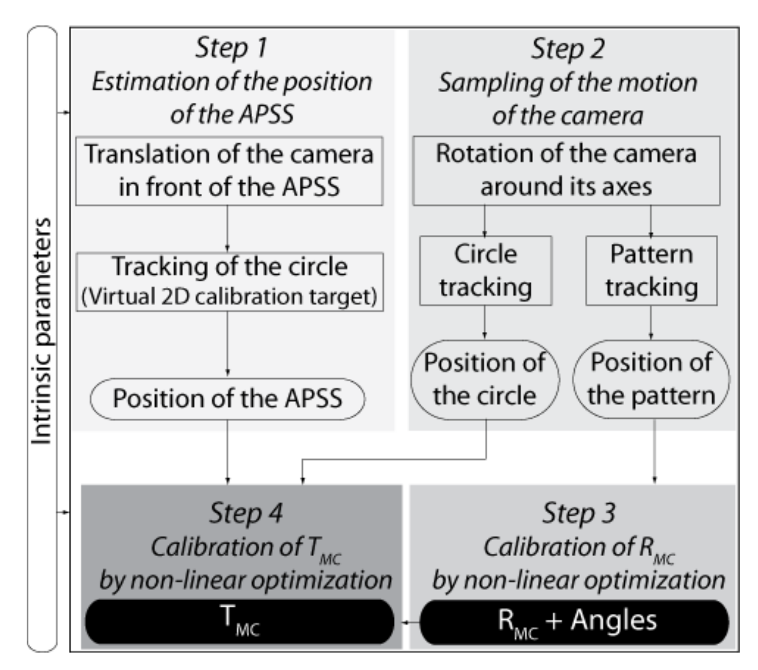
4.3.3. A Four-Step Procedure for Calibrating
The Four-step procedure for calibrating
is shown in
Figure 15. In this procedure, it is assumed that the intrinsic parameters of the cameras have been calibrated beforehand (see
Section 4.2). The procedure is presented for one camera only since it is similar for both cameras of the ASP.
The first step of the procedure for calibrating
consists of the estimation of the position
of the APSS in the reference frame of the camera in its initial configuration (i.e.,
in
Figure 6). This can be achieved by (
i) finding the frame transformation
expressing the position and orientation of the APSS in
, the reference frame of the camera, and (
ii) computing
, the position of the APSS in
using
.
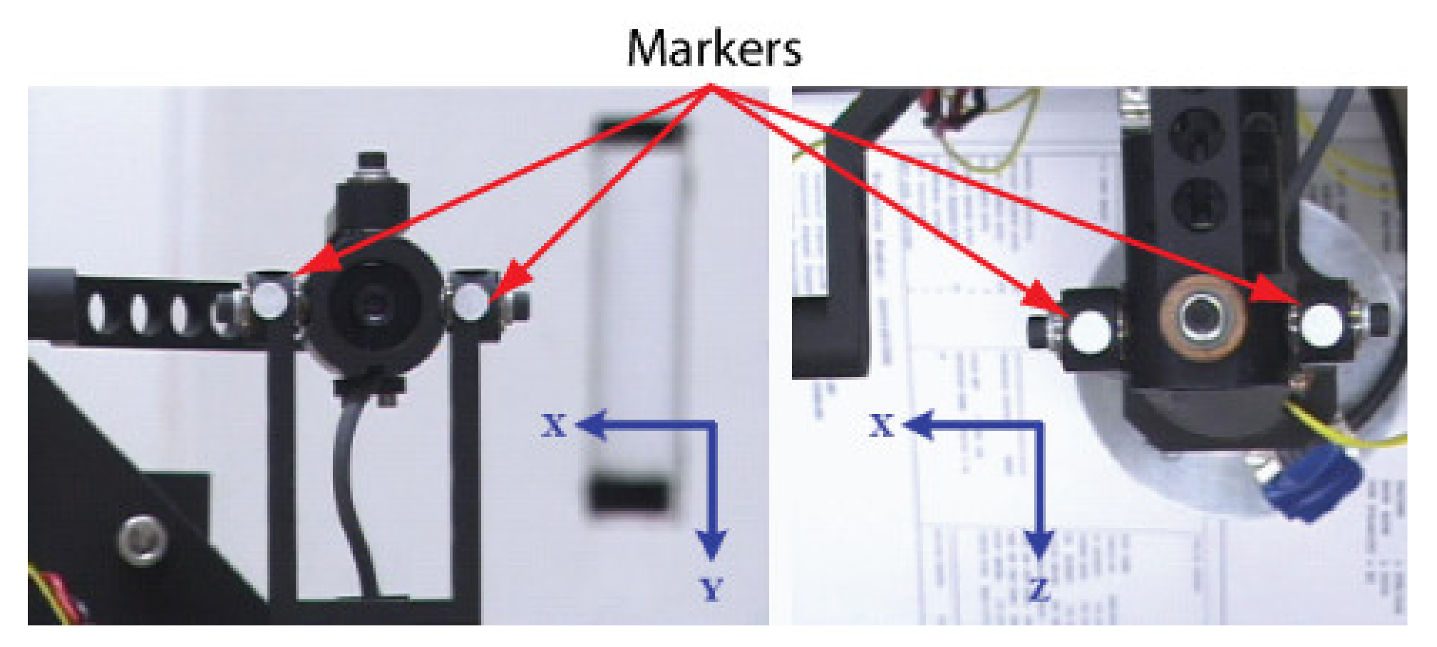
The approach starts by translating the APSS in front of the camera using two precision linear stages mounted at 90°, as shown in
Figure 16a. At least four different positions are required. For each position, an image of the APSS is acquired (with the plexiglass moving in front of it, see
Figure 16b for details of the experimental setup) and the center of gravity of the circle is computed with sub-pixel accuracy (see
Appendix A for details). The group of positions—centers of gravity pairs form a virtual calibration target mimicking the one shown in
Figure 5. Assuming the origin
of the reference frame attached to the “virtual” calibration target is located at the APSS and the orientation of its axes is along the translation stages, the problem of computing
stands as follows:
where
is the position of the center of gravity of the circle in the
ith image and
is the corresponding position of the camera set by the translation stages. The estimation of
is nothing but the procedure described above for the calibration of the pose of a camera with respect to a calibration target. Once
is known, the APSS is moved with the translation stages so that the image of the circle is located as much as possible at the center of the field of view on the image plane.
can then be computed. One way of doing this is to read the values of the translation stages, which provide the position
of the APSS in frame
, and then to find
with:
However, this approach is error-prone due to various measurement errors, which were found to have an adverse effect on the calibration of
. A better procedure is as follows. Let
be the coordinates of the center of gravity of the image of the circle on the image plane. The equation of the projector going from this point to the APSS is given by:
where
K is given by Equation (2). The APSS must be located along this projector and the following thus holds true for a scalar
α:
Now, the third column of
contains the components of the
Z-axis of the virtual calibration target expressed in frame
:
In addition,
, the translation component of
, corresponds to the position of the origin of
in frame
and thus provides a point belonging to the virtual calibration plane:
Knowing a point and the normal
to the virtual calibration plane, and knowing that
also lies on this plane, one can write:
Replacing Equation (35) in Equation (38) and solving for
gives:
This value for enables the computation of with Equation (35) and completes STEP 1.
In the above procedure, it is assumed that the linear translation stages are perfectly perpendicular, a condition that is difficult to meet in experimental conditions. It is possible to take the non-orthogonality between the translation axes into account in the calibration procedure. Doing so improves the quality of the estimation of
and, by the same token, the quality of the estimate for
. A method for taking this non-orthogonality into account in the calibration procedure is presented in
Appendix C.
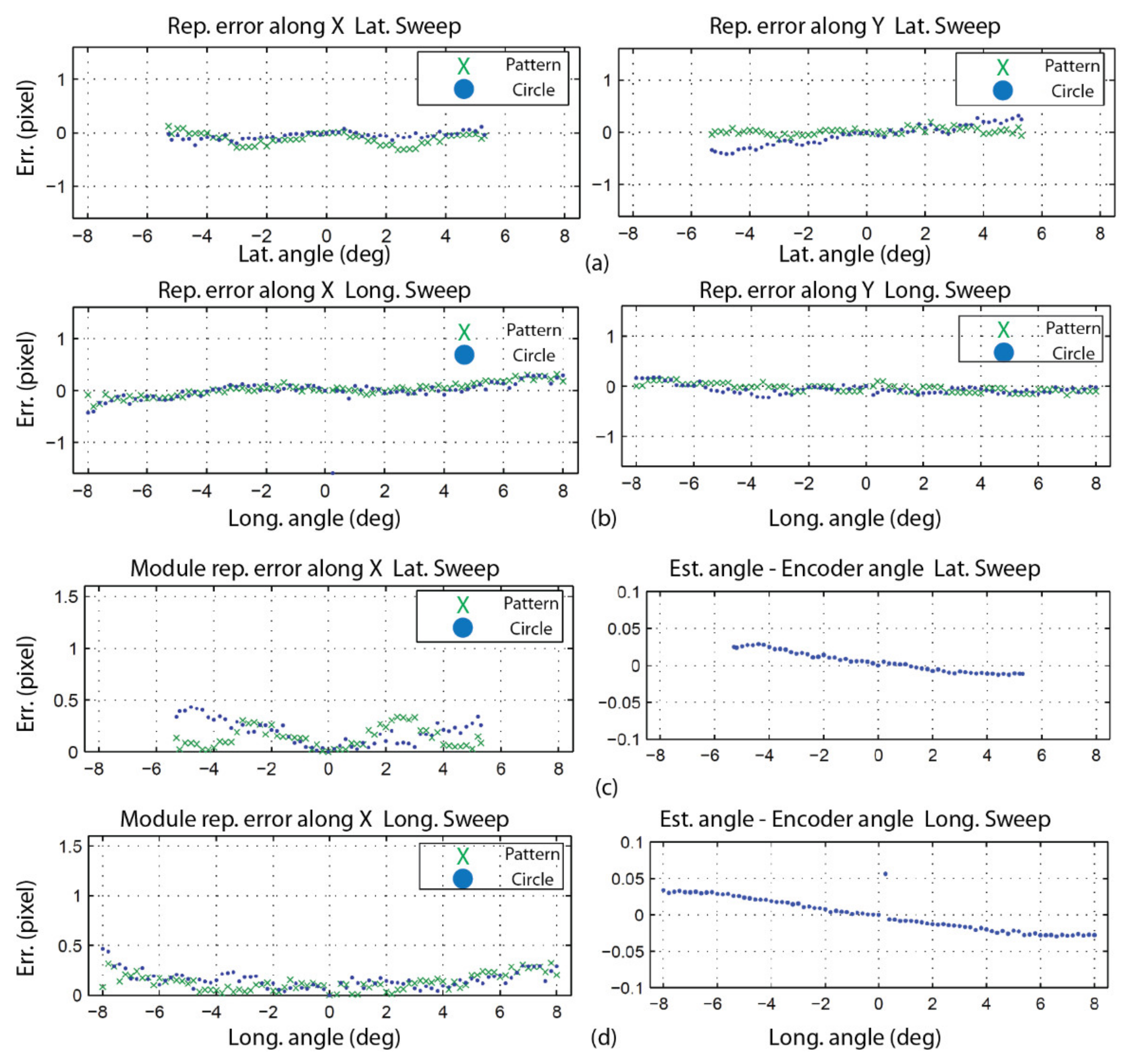
Once STEP 1 is complete, the next operation consists of acquiring two sets of images, one for each axis of the camera (this is repeated for both cameras of the ASP). The first series is acquired while the camera executes a longitudinal angular sweeping of the APSS (i.e., around axis Y) and the second one for a latitudinal sweeping of the APSS (around axis X), see
Figure 17a for a diagram of the longitudinal sweeping operation). For each sweeping operation around one axis, the other axis is kept at its initial position (
or
on
Figure 6) and the images of the circle (with the diffusing plexiglass in position) and the speckle pattern (with the diffusing plexiglass removed) are stored at each angular position. Since
, the rotations will cause the position of the geometric center of the circle to move by
(because of the rotation and translation of frame
in frame
) and the position of the speckle pattern circumscribed by the circle to move by
(because of the rotation of frame
). This behavior is shown in
Figure 18.
Once the images are acquired, they are processed for each angular position to find: (
i) the center of gravity of the circle and (
ii) the position of the speckle pattern. The approaches for computing these parameters are detailed in
Appendix A and
Appendix B, respectively. This information is used in Steps 3 and 4 of the calibration procedure.
STEP 3 aims at estimating
, the transform representing the
rotation component of
, using
, the displacement of the speckle pattern for each angular position
i imposed at STEP 2. The strategy consists of finding the orientation of the longitudinal and latitudinal axes of frame
in frame
, the reference frame of the camera. Knowing the orientation of these axes is all that is needed to estimate
since, according to the geometric model of each eye of the ASP (see
Figure 4 and
Figure 6), the latitudinal and longitudinal rotation axes correspond to axes X and Y of frame
. When the orientations of two orthogonal axes of a reference frame are known in another reference frame, the orientation of the reference frame itself is known. In other words, finding the orientation of the longitudinal and latitudinal axes of frame
in frame
allows finding
, the rotation component of frame
in frame
.
is simply obtained as
. Strictly speaking, the latitudinal and longitudinal axes found at STEP 3 are axes X and Y of frame
in frame
since these axes are the ones that are actuated by the motors; however, under the experimental conditions described at STEP 2, which impose that the rotations around each axis are performed when the other axis is kept in its initial position
, frame
is superimposed perfectly with frame
and the axes found are also those of frame
in frame
.
Before describing the non-linear optimization algorithm that is used for finding the orientation of the latitudinal and longitudinal axes of
in
, a geometric interpretation of the procedure and its relationship with the image acquisition process described at STEP 2 are presented first. Finding the axes (and their orientation) is achieved by imposing rotations of frame
in frame
. A single rotation is not enough since a rotation around any axis lying on a plane normal to the line joining the two vectors can bring a direction vector
to a new position
as shown in
Figure 17b).
However, only one axis can bring
to
and
(see
Figure 17d) with two successive rotations. It is why, at STEP 2, a longitudinal sweeping of the camera in front of the APSS is executed with the other axis in its initial position. The different angular positions
(with
) allow a direction vector
corresponding to a speckle point in the first image of the sweep to be brought to different directions
corresponding to the same speckle point that has moved by
due to the rotation (
Figure 13a,b). One way of finding the longitudinal axis (and latitudinal axis afterwards) would be to compute the intersection of the plane bringing
on
and the plane bringing
on
(and repeat this for all pairs of direction vectors
on
and
on
).
However, this approach was found to be sensitive to measurement noise. A much more accurate method consists of using non-linear optimization with a cost function directly linked to observations in the image (i.e., the speckle pattern and associated direction vectors). As shown in
Figure 17c, the non-linear optimization method formulates a hypothesis for the axis to be estimated and computes the angular displacements using this axis and the displacement of the speckle pattern from one image to the other. Using the hypothesis for the axis and the computed angular displacements, it is possible to find the estimates of direction vectors. Since
, the hypothesis for the axis may initially be far from the true axis, vectors
do not correspond to the true motion of the speckle pattern. The cost function uses these estimates and the direction vectors
measured in the images to generate a new estimate for the rotation axis until convergence. This procedure is now described formally.
The non-linear optimization procedure presented in
Figure 19a is used for estimating the orientation of the longitudinal and latitudinal axes. As shown in the figure, the rotation angles that were imposed on the agile eye at STEP 2 are estimated. Each rotation axis (latitudinal and longitudinal) is processed separately. A direction vector
(see
Figure 13c can be computed for each angular position of the camera. This vector is expressed in the reference frame of the camera (i.e.,
). The coordinates
of the reference point on the speckle pattern from which the vector originates can be expressed as coordinates on the normalized image plane with:
where
is the inverse of
in Equation (2). The components of the direction vector are obtained with the following equation (since this vector passes through the origin of the camera reference frame):
The point on the speckle pattern being used as a reference and being tracked at each angular position corresponds to direction vector
expressed in
, a fixed reference frame. According to the model of the agile eye (
Figure 4, left or right eye with
superimposed with
), the relation between
and
is given by (only rotations are considered here):
Although the matrix to be calibrated is
, the key matrix in Equation (42) is
since it is through this matrix that the camera is rotated because it models the parallel mechanism; however,
is unknown. As a matter of fact, in the optimization loop of
Figure 19a,
is assumed to be known and each iteration aims at refining this estimate as described next.
The focus on
is expressed explicitly by rewriting Equation (42):
with:
In Equation (44),
can be computed directly since
(and its inverse
), is assumed to be known. The reference direction vector
can also be computed with Equation (43) by considering that it is
, the direction vector for angular position
which leads to:
In the initial configuration (i.e., , ), and can be computed directly with the hypothesis for .
All that remains is to find matrices
allowing us to bring
on
and find the angles associated with each rotation of the agile eye. Based on the model of the agile eye and Equations (13) and (12), matrix
is given by (for each camera):
Strictly speaking, it is not possible to find
because only one equation (Equation (43)) is available to compute two unknowns (
and
). This explains why each axis was processed separately at STEP 2. Let us assume that only the rotations around the latitudinal axis are considered. In this case, X is the rotation axis and
since the rotation around Y is null. This leaves only one unknown that is computed with Equation (43). Projecting
and
on plane YZ, which is normal to axis X as shown in
Figure 17d, yields
and
. The angle between the projections can be found from their scalar product:
The value found for
can be used in Equation (46) to find
. The procedure is similar for rotations around the longitudinal axis (Y). Returning to
Figure 19a, the next operation consists of computing the reprojections of the direction vectors on the image plane using the current hypothesis for
, angles
, and matrices
. This starts by simulating the rotations of the agile eye for estimating the orientations of direction vectors in the reference frame of the camera with:
Direction vector
is a computation of the direction vector while
represents a measurement of the direction vector from the observation of the speckle pattern. When the optimization process is initiated, the hypothesis for
is likely to be far from its actual value and
and
are different. In Equation (48),
is given by Equation (45). The projection
of
on the image plane is given by:
while the projection
of
measured on the image plane is:
If
rotations are sampled for axis
a, the error vector between computed values and measured values of direction vectors is defined as:
The Levenberg–Marquardt non-linear optimization algorithm uses this error vector to minimize the following cost function:
where
are the parameters defining
,
is the projection of the direction vector of the speckle pattern measured for camera angular position
i,
is the number of sampled angular positions for axis
a,
is the projection of the direction vector of the speckle pattern computed with the current hypothesis for
, and
is the projection of the reference direction vector.
In the preceding procedure, data collected from rotations around each axis have been processed independently up to Equation (51). The results related to each axis need to be combined in the cost function described by Equation (52) to optimize all parameters of simultaneously. Doing so instead of estimating the orientation of each axis of rotation independently makes sure that the orthogonality constraint between the two rotation axes is met.
The last step for the calibration of
is to estimate the translation component
of the transform by non-linear optimization. The procedure for calibrating
is described in
Figure 19b. It accepts as inputs: (
i) the position of the APSS in the reference frame of the camera found at STEP 1, (
ii) the position of the center of gravity of the circles (sampled at STEP 2 and computed with the approach described in
Appendix A for different angular positions of the camera), (
iii)
found at STEP 3, (
iv) initial values for the three elements of
, and (
v) the values of the angles for the angular positions of the camera.
The procedure for computing the values of the angles for the angular positions of the camera is the one that was used in the non-linear optimization algorithm for finding at STEP 3 (using Equations (42)–(47), but this time, the estimate for is used).
The above information is fed to a Levenberg–Marquardt non-linear optimization algorithm, which now refines the translation parameters of
using the measured and computed reprojections of the center of gravity of the circles for each angular position. The reprojections are computed as follows. The position of the APSS in frame
is:
In Equation (53),
since the camera is at its initial angular position. We thus have
where
is the matrix found at STEP 3 and
is assumed to be known since it is the hypothesis. With
known, the position of the source in the reference frame of the camera for each angular position is given by:
with
given by Equation (11). Again, each axis is processed independently, which means that either
or
. Finally, the coordinates of the reprojected center of gravity of the circle on the image plane are given by:
The error vector for axis
a is given by:
and is used to minimize:
where
. In Equation (58),
is the position of the projection of the center of gravity of the circle being observed at angular position
i,
is the number of angular positions of the camera, and
is the projection of the center of gravity of the circle computed with the current hypothesis for
.
The significant advantage of the calibration approach using speckle metrology is that it uncouples the estimation of and completely since different (and independent) image information operations (displacement of the speckle pattern for and displacement of the center of gravity for ) are used to estimate each transform. Consequently, a small rotation cannot be confused for a small translation and vice-versa.


