Abstract
This research presents a brain-computer interface (BCI) framework for brain signal classification using deep learning (DL) and machine learning (ML) approaches on functional near-infrared spectroscopy (fNIRS) signals. fNIRS signals of motor execution for walking and rest tasks are acquired from the primary motor cortex in the brain’s left hemisphere for nine subjects. DL algorithms, including convolutional neural networks (CNNs), long short-term memory (LSTM), and bidirectional LSTM (Bi-LSTM) are used to achieve average classification accuracies of 88.50%, 84.24%, and 85.13%, respectively. For comparison purposes, three conventional ML algorithms, support vector machine (SVM), k-nearest neighbor (k-NN), and linear discriminant analysis (LDA) are also used for classification, resulting in average classification accuracies of 73.91%, 74.24%, and 65.85%, respectively. This study successfully demonstrates that the enhanced performance of fNIRS-BCI can be achieved in terms of classification accuracy using DL approaches compared to conventional ML approaches. Furthermore, the control commands generated by these classifiers can be used to initiate and stop the gait cycle of the lower limb exoskeleton for gait rehabilitation.
1. Introduction
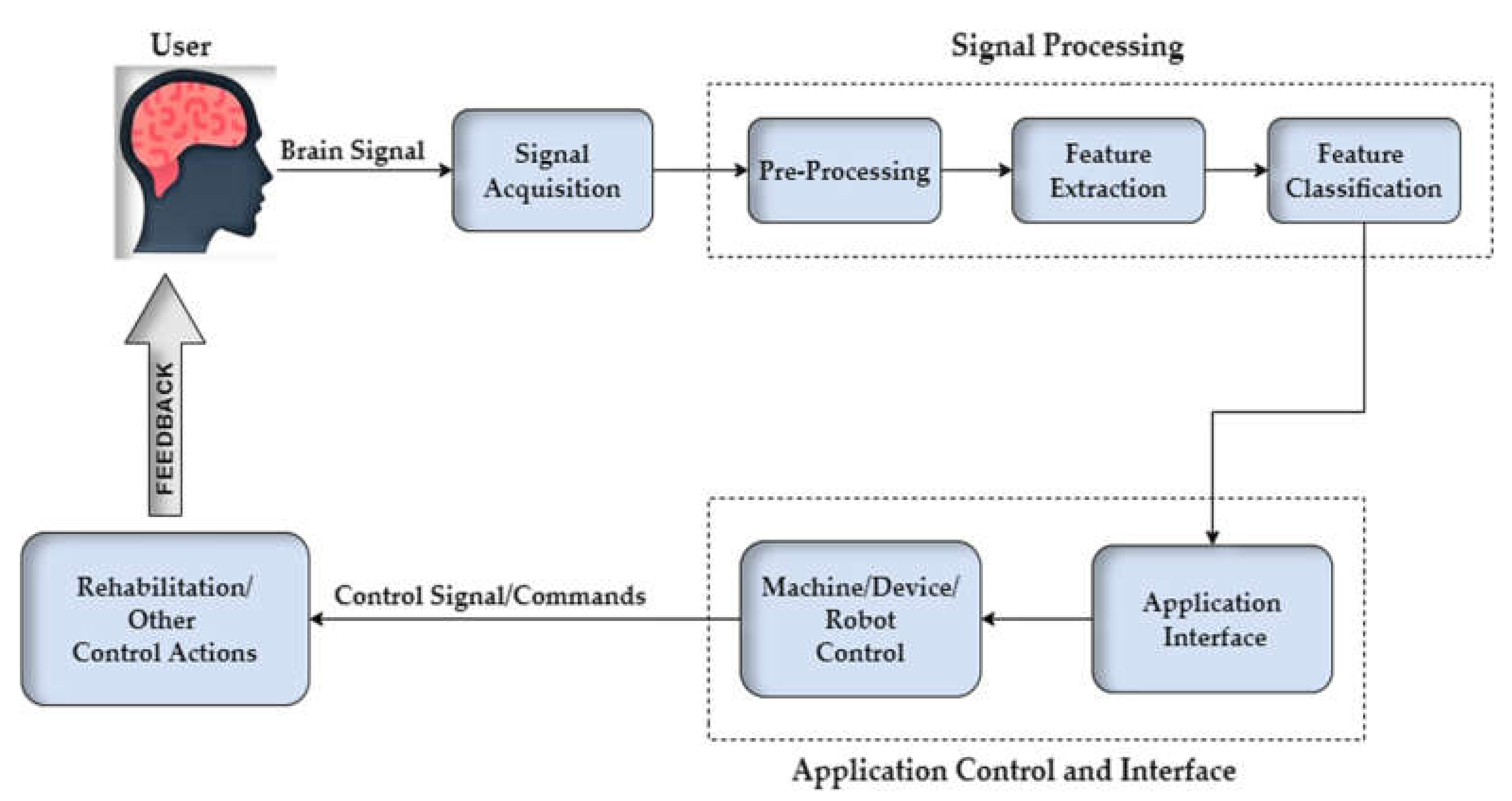
The world has been striving to create a communication channel based on signals obtained from the brain. A brain-computer interface (BCI) is a communication system that provides its users with control channels independent of the brain’s output channel to control external devices using brain activity [1,2]. The BCI system was first introduced by Vidal in 1973 in which he proposed three assumptions regarding BCI, including analysis of complex data in the form of small wavelets [3]. A typical BCI system consists of five stages, as shown in Figure 1. The first stage is the brain-signal acquisition using a neuroimaging modality. The second is preprocessing those signals as they contain physiological noises and motion artefacts [4]. The third stage is feature extraction in which meaningful features are selected [5]. These features are then classified using suitable classifiers. The final stage is the application interface in which the classified BCI signals are given to an external device as a control command [6].

Figure 1.
Basic design and operation of the brain-computer interface (BCI)-based control.
Researchers have been using different techniques to acquire brain signals [7]. These techniques include electroencephalography (EEG), functional near-infrared spectroscopy (fNIRS), magnetoencephalography (MEG), and functional magnetic resonance imaging (fMRI) [8]. EEG is a technique used to analyze brain activity by measuring changes in the electrical activity of the active neurons in the brain [9], while MEG measures the changes in magnetic fields associated with the brain’s electrical activity changes [10]. fMRI is another modality for analyzing brain function by measuring the localized changes in cerebral blood flow stimulated by cognitive, sensory, or motor tasks [11,12]. In this study, we will only be dealing with fNIRS-BCI. fNIRS is a non-invasive optical neuroimaging technique that measures the concentration changes of oxy-hemoglobin (ΔHbO) and deoxy-hemoglobin (ΔHbR) that are associated with the brain activity stimulated, when participants perform experiments, such as arithmetic tasks, motor imagery, motor execution, etc. [13]. It is a non-invasive, portable and easy-to-use brain imaging technique that helps study the brain’s functions in the laboratory, naturalistic, and real-world settings [14]. fNIRS consists of near-infrared light emitter detector pairs. The emitter emits light with several distinct wavelengths absorbed in the subject’s scalp, consequently causing scattered photons; while some of them are absorbed, the others disperse and pass through the cortical areas where HbO and HbR chromophores absorb the light and have different absorption coefficients. The concentration of HbO and HbR changes along the photon path in consideration of the modified Beer-Lambert law [15].
In the recent decade, the research on fNIRS-BCI has increased enormously, and new diverse techniques, particularly in its applications, may grow exponentially over the following years [16]. One of the significant fields of fNIRS application is cognitive neuroscience, particularly in real-world cognition [17], neuroergonomics [18], neurodevelopment [19], neurorehabilitation [20], and in social interactions. fNIRS-BCI can provide a modest input for BCI systems in the real time, but improvements are required for this system as there is the difficulty faced with the collection and interpretation of the data for classifiers due to noise in the data and subject variations [21].
Well-designed wearable assistive devices for rehabilitation and performance augmentation purposes have been developed that run independently of physical or muscular interventions [22,23,24]. Recent studies focus on acquiring the user’s intent through brain signals to control these devices/limbs [25,26,27]. In assistive technologies, the fNIRS-BCI system is a suitable technique for controlling exoskeletons and wearable robots by using intuitive brain signals instead of being controlled manually by various buttons in order to get the desired postures [28]. In addition, it has a better spatial resolution, fewer artefacts, and acceptable temporal resolution, which makes it a suitable choice for rehabilitation and mental task applications [29].
To find the best machine-learning (ML) method for fNIRS-based active-walking classification, a series of experiments with various ML algorithms and configurations were conducted; the classification accuracy achieved was above 95% [30] for classifying 1000 samples using different ML algorithms, such as random forest, decision tree, logistic regression, support vector machine (SVM) and k-nearest neighbor (k-NN). In order to achieve minimum execution delay and minimum computation cost for an online BCI system, linear discriminant analysis (LDA) was used with combinations of six features for walking intention and rest tasks [31].
The traditional method of extracting and selecting acceptable features can result in performance degradation. In contrast, deep neural networks (DNNs) can extract different features from raw fNIRS signals, nullifying the need for a manual feature extraction stage in the BCI system development, but limited studies are available so far [32,33].
Convolutional neural network (CNN) is a deep-learning (DL) approach that can automatically learn relevant features from the input data [34]. In a study, CNN architecture was compared to conventional ML algorithms, and CNNs performed better in terms of classification with an average classification accuracy of 72.35 ± 4.4% for the four-class motor imagery fNIRS signals [35]. CNN-based time series classification (TSC) methods to classify fNIRS-BCI are compared with ML methods, such as SVM. The results showed that the CNN-based methods performed better in terms of classification accuracy for left-handed and right-handed motor imagery tasks and achieved up to 98.6% accuracy [36].
Time-series data can be handled more precisely using long short-term memory (LSTMs) modules. In a study, four DL models were evaluated including multilayer perceptron (MLP), forward and backward long short-term memory (LSTMs), and bidirectional LSTM (Bi-LSTM) for the assessment of human pain in nonverbal patients, and Bi-LSTM model achieved the highest classification accuracy of 90.6% [37]. Using the LSTM network, large time scale connectivity can be determined with the help of the InceptionTime neural network, which is an attention LSTM neural network utilized for the brain activations of mood disorders [38]. A recent study assessed four-level mental workload states using DNNs, such as CNNs and LSTM for fNIRS-BCI system, with average classification accuracies of 87.45% and 89.31% [39].
This study contributes to the development of a neurorehablitation tool in the gait training of elderly and disabled people. The main objective of this study is to compare two classification approaches, ML and DL, to achieve high performance in terms of classification accuracy on the time-series fNIRS data. The complete summary of the methods employed in this research is depicted in Figure 2.
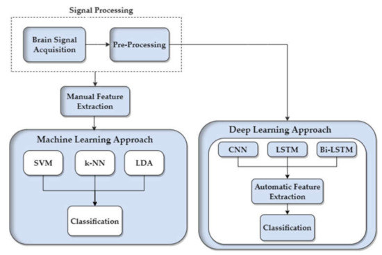
Figure 2.
Time-series functional near-infrared spectroscopy (fNIRS) signal classification for walking and rest tasks using conventional machine-learning (ML) and DL algorithms. Signal processing and feature engineering followed by classification using ML and DL approaches.
2. Materials and Methods
2.1. Experimental Paradigm
Nine healthy right-handed male subjects of 27 ± 5 median age were selected. The subjects had no history of motor disability or any visual neurological disorders affecting the experimental results. fNIRS-based BCI signals were acquired from the primary motor cortex (M1) in the left hemisphere for self-paced walking [40]. Before the start of each experiment, the subjects were asked to take a rest for 30 s in a quiet room to establish the baseline condition; it was followed by 10 s of walking on a treadmill, followed by 20 s of rest while standing on the treadmill. At the end of each experiment, a 30 s rest was also given for baseline correction of the signals. Each subject performed 10 trials, as shown in Figure 3. Excluding the initial (30 s) and final (30 s) of rest, the total length of each experiment was 300 s for each subject. All the experiments were conducted in accordance with the latest Declaration of Helsinki and approved by the Institutional Review Board of Pusan National University, Busan, Republic of Korea [41].
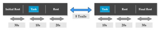
Figure 3.
Experimental paradigm with experimental 10 trials with initial and final 30 s rest.
2.2. Experimental Configuration
In this study a multi-channel continuous-wave imaging system (DYNOT: Dynamic Near-infrared Optical Tomography; NIRx Medical Technologies, NY, USA) was used to acquire the brain signals, which operate on two wavelengths, 760 and 830 nm, with a 1.81 Hz sampling frequency. Four near-infrared light detectors and five sources (total of nine optodes) were placed on the left hemisphere of the M1 with 3 cm of distance between a source and a detector [42]. A total of twelve channels were formed in accordance with the defined configuration, as shown in Figure 4.
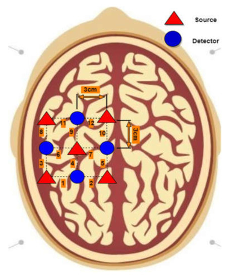
Figure 4.
Optode placement on the left hemisphere of the motor cortex with channel configuration using 10–20 international system.
2.3. Signal Acquisition
The acquired light intensity signals from the left hemisphere of the M1 were first converted into oxy- and deoxy-hemoglobin concentration changes (, and ) using the modified Beer-Lambert law [43].
where and are the concentration changes of HbO and HbR in [μM], A(t, ) and A(t, ) are the absorptions at two different instants, is the emitter–detector distance (in millimeters), d is the unitless differential path length factor (DPF), and and are the extinction coefficients of HbO and HbR in [μM−1 cm−1].
2.4. Signal Processing
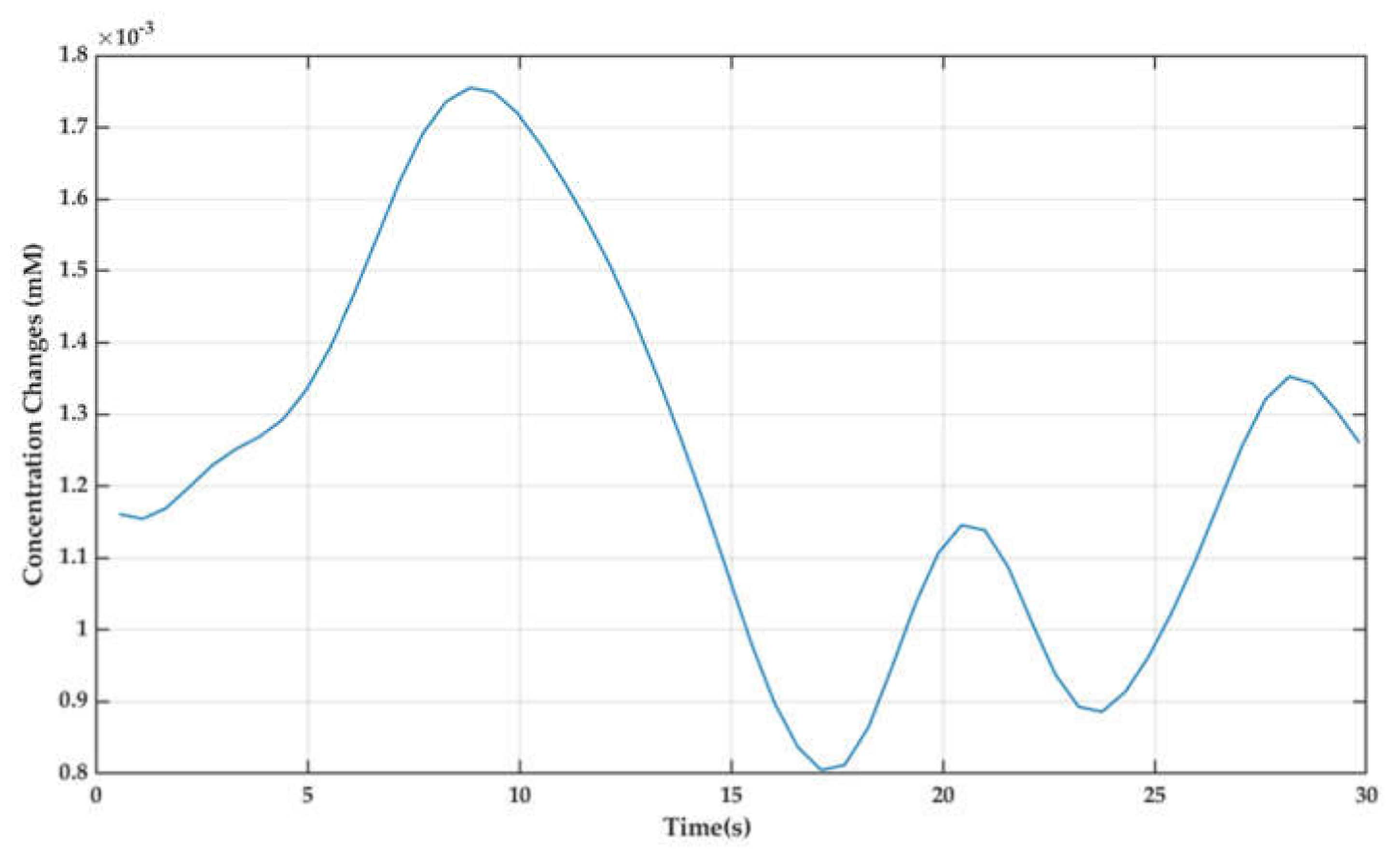
After obtaining oxy-hemoglobin concentration changes ( and ), the brain signals acquired were filtered with suitable filters using the modified Beer-Lambert law. In order to minimize the physiological or instrumental noises, such as heartbeat (1–1.5 Hz), respiration (~0.5 Hz), Mayer waves (blood pressure), artefacts, and others, the signals were low-pass filtered at a cut-off frequency of 0.5 Hz and a high-pass filter with cut-off frequency of 0.01 Hz [44]. The filter used for signals were hemodynamic response (hrf) using NIRS-SPM toolbox [45]. The averaged signal for task and rest of subject 1 after filtering is shown in Figure 5.
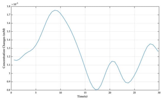
Figure 5.
Averaged signal for task and rest of subject 1.
2.5. Feature Extraction
For the conventional ML algorithms, five different features of filtered signals were extracted using the spatial average for all 12 channels. Five statistical properties (mean, variance, skewness, kurtosis, and peak) of the averaged signals were calculated for the entire task and rest sessions. In this study, a feature combination of signal mean, signal peak, and signal variance a was used for the ML classifiers. This specific combination was selected based on the higher classification accuracies that were obtained using these features [46,47].
For the mean, the equation was as follows:
where N is the total number of observations, and is the across each observation. For signal variance, the calculation was as follows:
where n is the sample size, is the ith element of the sample, and is the mean of the sample. To calculate signal peak, the max function in MATLAB® was used.
3. Classification Using Machine-Learning Algorithms
3.1. Support Vector Machine (SVM)
SVM is a commonly used classification technique suitable for fNIRS-BCI systems for handling high-dimensional data [48,49]. In supervised learning, the SVM classifier creates hyperplanes to maximize the distance between the separating hyperplanes and the closest training points [50]. The hyperplanes, known as the class vectors, are called support vectors. The separating hyperplane in the two-dimension features space is given by:
where b is a scaling factor, and . The optimal solution, r*, that is the distance between the hyperplane and the nearest training point(s) is maximized by minimizing the cost function. The optimal solution, r* is given by the equation.
Minimize
Subject to
where represents the class label for the ith sample, T is the transpose, and n is the total number of samples, = . where and , , C is the trade-off parameter between the margin and error, and is the training error.
3.2. k-Nearest Neighbor (k-NN)
k-NN predicts the test sample’s category; the k value represents the number of neighbors considered and classifies it in the same class as its nearest neighbor based upon the largest category probability [51]. Euclidean distance is the distance between the trained and the test object given by the equation.
where n is the n-space, and are two points in the Euclidean n-space, and are the two vectors, stating from the origin of the space.
k-NN is a widely used efficient classification method for BCI applications because of its low computational requirements and simple implementation [52,53].
3.3. Linear Discriminant Analysis (LDA)
LDA has discriminant hyperplanes to separate classes from each other. LDA performs well in various BCI systems because of its simplicity and execution speed [54]. It minimizes the variance of the class and maximizes the separation between the mean of the class by maximizing the Fisher’s criterion [55]. The equation for Fisher’s criterion is given by:
where and are the between-class and within-class scatter matrices given as:
where denotes samples, and are the group means of classes and , respectively.
4. Classification Using Deep-Learning Algorithms
fNIRS signal classification with conventional ML methods is composed of local and global feature extraction, e.g., independent component analysis (ICA) and principal component analysis (PCA), selection of possible features, their combinations, and dimensionality reduction, which leads to the biasness and overfitting of the data [56]. It is because of these limitations a large amount of time is consumed in the mining and preprocessing of the data [57].
The BCI classification task can avoid local filtering, noise removal, and manual local feature extraction by utilizing DL algorithms as an alternative to avoid the need for manual feature engineering, data cleaning, analysis, transformation, and dimensionality reduction before feeding it to the learning machines [58]. Extracting and selecting appropriate features is critical with fNIRS-BCI signals, and the multi-dimensionality and complexity of fNIRS signals make it ideal for DL algorithms to work with.
4.1. Convolutional Neural Networks (CNNs)
CNNs are a type of neural networks that are capable of automatically learning appropriate features from the input fNIRS time-series data. CNNs consist of several layers, such as the convolutional layer, pooling layer, fully connected layer, and output layer [59]. The input fNIRS time-series data (the changes in the HbO concentrations) across all the channels are passed through CNN layers. The convolutional layer contains filters that are known as convolution kernels to extract features. CNN minimizes the classification errors by adjusting the weight parameters of each filter using forward and backward propagation.
The convolution operation is the sliding of a filter over the time series, which results in activation maps also known as feature maps that stores the features and patterns of the fNIRS data [60]. Convolution operation for time stamp t is given by the equation:
where C is the output of a convolution (dot product) on a time series, X, of length, T, with a filter, , of length, l, b is a bias parameter, and f is a non-linear function, such as the rectified linear unit (ReLU).
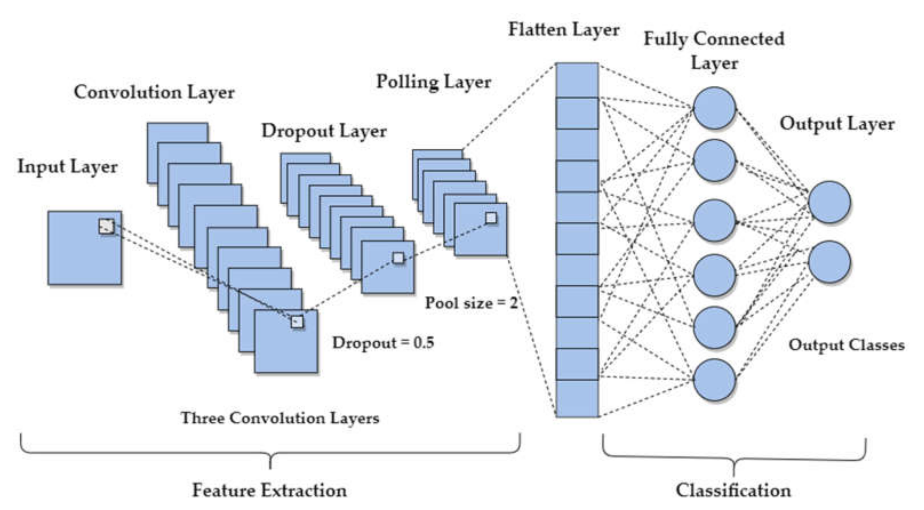
After the convolutional layer, we have a pooling layer that downsamples the spatial size of the data and also reduces the number of parameters in the network [61]. The pooling layer is followed by a fully connected layer, as shown in Figure 6 in which each data point is treated as a single neuron that outputs the class scores, and each neuron is connected to all the neurons in the previous layer [62].

Figure 6.
Convolutional neural network (CNN) model with convolutional layer, dropout layer, pooling layer, flatten layer, fully connected layer, and output layer.
The proposed CNN model consists of the input layer, three one-dimensional convolutional layers, max-pooling layers, dropout layers, a fully connected layer, and an output layer. The three convolutional layers contain filters 128, 64, 32 with a kernel size of 3, 5, 11, respectively. A dropout layer of 0.5 ‘dropout ratio’ was added after each convolutional layer to avoid overfitting, followed by a pooling layer with a stride of two. The input fNIRS time-series data after passing through a number of convolutional, max-pooling, and dropout layers is flattened and fed into the fully connected layers for the purpose of classification. The fully connected layer of 100 units is incorporated with ReLU activation. The output layer consists of two neurons corresponding to the two classes with Softmax activation. The optimization technique used was Adam with a batch size of 150 and 500 number of epochs.
4.2. Long Short-Term Memory (LSTM) and Bi-LSTM
LSTM is a DL algorithm that can achieve high accuracies in terms of classification, processing, and forecasting predictions on the time-series fNIRS data. LSTMs have internal mechanisms called gates that can regulate the flow of information [63]. These gates, such as forget gate, input gate, and output gate, can learn which data in a sequence are necessary to keep or throw away [64]. By doing that, it can pass relevant information down the long chain of sequences to make predictions. The equations for forget gate (), input gate () and output gate () are given by:
where , , and are the weight matrices of forget, input, and output gates, respectively, and is the hidden state.
These gates contain sigmoid and Tanh activations to help regulate the values flowing through the network [65]. General sigmoid function is given by:
where is the x-value of the sigmoid midpoint, e is the natural logarithm base, and k is the growth rate.
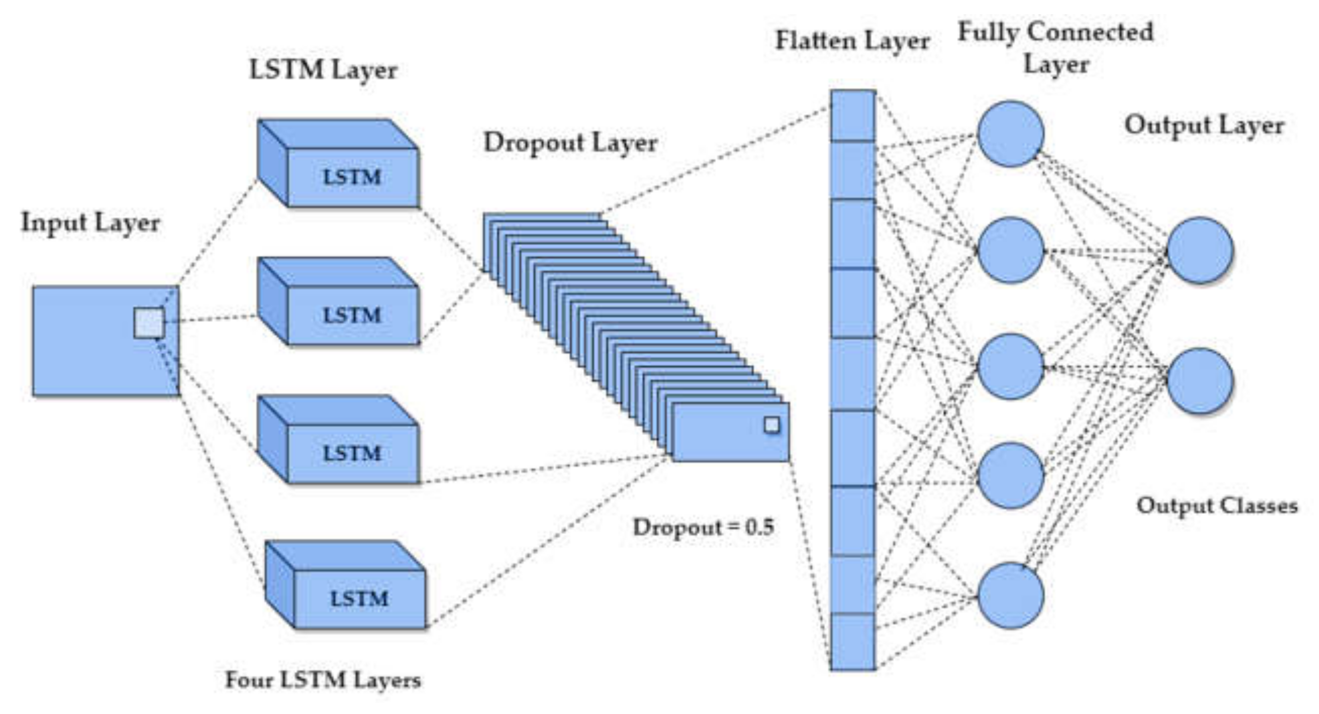
For LSTM the data has to be reshaped because it expects the data in the form of (m × k × n), where m is the number of samples, n refers to the number of fNIRS channels (12 channels), and k refers to the time steps. The proposed LSTM model consisted of an input layer, four LSTM layers, a fully connected layer, and an output layer, as shown in Figure 7. A dropout layer of 0.5 ‘dropout ratio’ was added after the LSTM layers to avoid overfitting. The output from the dropout layer is flattened and fed to the fully connected layer of 64 units, also known as the dense layer, and incorporated with ReLU activation. Finally, an output layer consists of two neurons corresponding to the two classes with Softmax activation. The early-stopping technique was used to avoid overfitting with the patience of 50; a batch size of 150 over 500 epochs with Adam optimization technique.
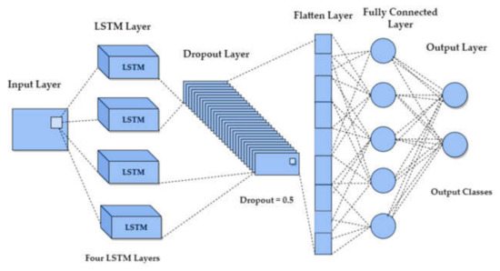
Figure 7.
Long short-term memory (LSTM) model with four LSTM layers, dropout layer, flatten layer, fully connected layer, and output layer.
Bi-LSTM models are a combination of both forward and backward LSTMs [66]. These models can run inputs in two ways, from past to future and from future to past and have both forward and backward information about the sequence at every time step [67]. Bi-LSTM differs from conventional LSTMs as they are unidirectional, and with bidirectional, we are able at any point in time to preserve information from both past and future, which is why they perform better than conventional LSTMs [68].
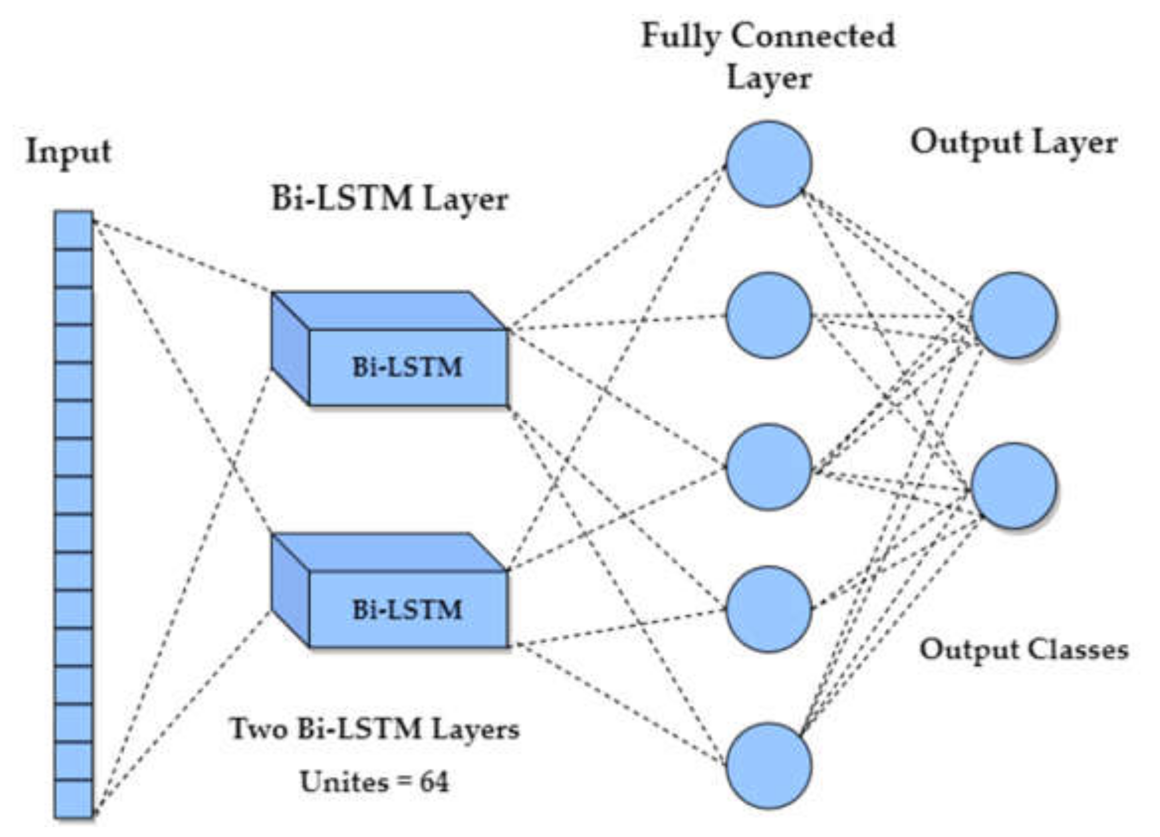
The proposed Bi-LSTM model consisted of two Bi-LSTM layers with 64 hidden units, a fully connected layer, and an output layer, as shown in Figure 8. The fully connected layer of 64 units is employed with ReLU activation, and the output layer consists of two neurons corresponding to the two classes with Softmax activation.

Figure 8.
Bidirectional LSTM (Bi-LSTM) model with two Bi-LSTM layers with 64 units, fully connected layer, and output layer.
5. Results
The results evaluated for all the methods used in this study are presented in this section, including the validation of the methods. ML algorithms (SVM, k-NN, and LDA) were performed on MATLAB® 2020a Classification Learner App, whereas DL algorithms (CNN, LSTM, and Bi-LSTM) were performed on Python 3.7.12 on Google Colab using Keras models with TensorFlow.
5.1. Classification Accuracy of Machine-Learning Algorithms
For ML algorithms, five features (signal mean, signal variance, signal skewness, signal kurtosis, and signal peak) across all 12 channels of filtered signals were spatially calculated. Three feature combinations that were signal mean, signal variance, and signal peak yielded the best results. The manually extracted features from fNIRS data of walking and rest states of nine subjects are fed to the three conventional ML algorithms, SVM, k-NN, and linear LDA, and the highest accuracies obtained were 78.90%, 77.01%, and 66.70% across 12 channels, respectively, as given in Table 1.

Table 1.
Accuracy of conventional machine-learning (ML) algorithms, k-nearest neighbor (k-NN), support vector machine (SVM), and linear discriminant analysis (LDA) for all nine subjects.
To curb overfitting, 10-fold cross-validation was used for the training of the models. The accuracy of conventional ML algorithms for all nine subjects is shown in a bar graph in Figure 9.
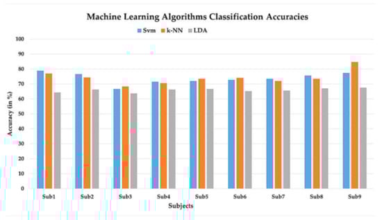
Figure 9.
Machine-learning (ML) classifier accuracies (in %) for nine subjects. The ML classifiers are support vector machine (SVM), k-nearest neighbor (k-NN), and linear discriminant analysis (LDA).
5.2. Classification Accuracy of Deep Learning Algorithms
To evaluate the deep-learning models, the dataset was initially split into an 80:20 ratio, the training set (80%) and the testing set (20%). The training set used for DL methods in this study has 12 feature dimensions. The learning performance of the algorithm is affected by the size of the training set, which is why 20% of the validation set were employed for each subject since the larger training set usually provides higher classification performance [69]. Although, for CNN, a smaller number of samples after the 30%validation set also attained classification accuracy reaching 90%. The pre-processed fNIRS data of walking and rest states of nine subjects is fed to the three DL algorithms, CNN, LSTM, and Bi-LSTM; the highest classification accuracies obtained were 95.47%, 95.35%, and 95.54% across 12 channels, respectively. The classification accuracy of DL algorithms for all nine subjects is shown in a bar graph in Figure 10.
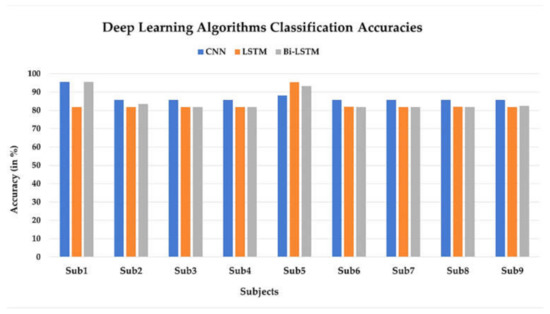
Figure 10.
Deep-learning (DL) classifier accuracies (in %) for nine subjects. The DL classifiers are convolutional neural network (CNN), long short-term memory (LSTM), and bidirectional LSTM (Bi-LSTM).
All the DL models (CNN, LSTM, and Bi-LSTM) were compiled with the metric “accuracy”, which is the measure of the number of correct predictions from all the predictions that were made. To further evaluate the effectiveness of the model, model “precision”, which is the number of positive predictions divided by the total number of positive predicted values and model “recall”, which is the number of actual positives divided by the total number of positive values were also calculated. Accuracy, precision, and recall of DL algorithms are summarized in Table 2, Table 3 and Table 4. The loss function used for the models was “categorical cross-entropy” which is a measure of prediction error, and the optimization technique used was “Adam optimizer”. In order to avoid overfitting, early-stopping technique was used to halt the training when the error during the last 50 epochs is not reduced. Learning rate of 0.001 and decay factor of 0.5 were used in all DL models.
Table 2.
Accuracy, precision, and recall of deep-learning (DL) algorithm, convolutional neural network (CNN) for all nine subjects.
Table 3.
Accuracy, precision and recall of deep learning (DL) algorithm, long short-term memory (LSTM) for all nine subjects.
Table 4.
Accuracy, precision and recall of deep learning (DL) algorithm, bidirectional LSTM (Bi-LSTM) for all nine subjects.
To evaluate the statistical significance of ML and DL methods, a t-test was performed for the best performing DL method (CNN) and all the other five classifiers accuracies, as shown in Table 5 The results of these statistical tests showed significant improvement of classification accuracy for the proposed DL method (p < 0.008) and the null hypothesis, meaning no statistical significance was rejected.
Table 5.
Statistical significance between CNN and all other five classifiers accuracies.
5.3. Validation
For the purpose of validation of the proposed methods, the analysis was also performed on an open-access database containing fNIRS brain signals ( and ) for the dominant foot tapping vs. rest [70]. The analysis was performed for 20 subjects with 25 trials for each subject. By applying the ML methods (SVM, k-NN, and LDA) on the fNIRS dataset for the dominant foot tapping vs. rest tasks, the average classification accuracies were estimated at 66.63%, 68.38%, and 65.96%, respectively, while for DL methods (CNN, LSTM, and Bi-LSTM) the average classification accuracies were estimated at 79.726%, 77.21%, and 78.97%, respectively. The students’ t-test showed significantly higher performance (p < 0.008) for the proposed DL method. The results obtained from the validation dataset also confirmed the high performance of the proposed DL methods over the conventional ML methods.
6. Discussion
Around the world, there are a substantial number of people that have gait impairment and permanent disability in their lower limbs [71]. In the recent decade, the development of wearable/portable assistive devices for mobility rehabilitation and performance augmentation focuses on acquiring the user’s intent through brain signals to control these devices/limbs [72]. In the field of assistive technologies, the fNIRS-BCI system is a relatively suitable technique for the control of exoskeletons and wearable robots by using intuitive brain signals instead of being controlled manually by various buttons to get the desired postures [28,31]. It has a better spatial resolution, fewer artefacts, and acceptable temporal resolution, which makes it a suitable choice for rehabilitation and mental task applications [29,73]. High accuracy BCI systems are to be designed in order to improve the quality of life of people with gait impairment since any misclassification can probably result in a serious accident [56]. To achieve this, the proposed DL and conventional ML methods are investigated for a state-of-the-art fNIRS-BCI system. The control commands generated through these models can be used to initiate and stop the gait cycle of the lower limb exoskeleton for gait rehabilitation.
Researchers have been exploring different ways to improve the classification accuracies by using different feature extraction techniques, feature combinations, or by using different machine-learning algorithms [30]. In a study, six feature combinations, signal mean (SM), signal slope (SS), signal variance (SV), slope kurtosis (KR), and signal peak (SP) have been used for walking and rest data, and the highest average classification accuracy of 75% was obtained from SVM using the hrf filter [31]. In this study, we used three feature combinations of the signal mean, signal variance, and signal peak, and the accuracy obtained from SVM using these features were 73.91%. In a recent study, four-level, mental workload states were assessed using the fNIRS-BCI system by utilizing DNNs, such as CNN and LSTM, and the average accuracy obtained using CNN was 87.45% [39]. Our study achieved almost the same average classification accuracy for CNN with 87.06% for two-class motor execution of walking and rest tasks.
CNN generally refers to a two-dimensional CNN used for image classification, in which the kernel slides along two dimensions on the image data. Recently, researchers have started using deep learning for fNIRS-BCI and bioinformatics problems and have achieved good performances using 2-D CNNs [35,74]. However, in this study, we have considered the one-dimensional CNN for time series fNIRS signals of motor execution tasks and reached a satisfactory classification accuracy. The highest average classification accuracy obtained in this study is 88.50%. For time-series fNIRS data, LSTMs and Bi-LSTMs can achieve high accuracy in terms of classification, processing, and forecasting predictions. In a study for assessing human pain in nonverbal patients, LSTM and Bi-LSTM models were evaluated, and the Bi-LSTM model achieved the highest classification accuracy of 90.6% [37]. In another study, the LSTM based conditional generative adversarial network (CGAN) system was analyzed to determine whether the subject’s task is left-hand finger tapping, right-hand finger tapping, or foot tapping based on the fNIRS data patterns, and the classification accuracy obtained was 90.2%. In the present study, the highest accuracy achieved on any subject with LSTM and Bi-LSTM is 95.35% and 95.54%, respectively, across all 12 channels. The comparison of the average accuracies obtained using ML and DL approaches is shown in a bar graph in Figure 11.
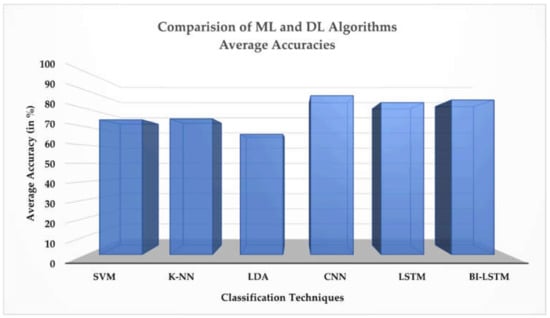
Figure 11.
Comparison between machine-learning (ML) classifiers (support vector machine (SVM), k-nearest neighbor (k-NN), and linear discriminant analysis (LDA)) and deep-learning (DL) classifiers (convolutional neural network (CNN), long short-term memory (LSTM), and bidirectional LSTM (Bi-LSTM)) based on average accuracies.
7. Conclusions
In this study, two approaches, ML and DL, are investigated to decode two-class data of walking and rest tasks to obtain maximum classification accuracy. The DL approaches proposed in this study, CNN, LSTM, and Bi-LSTM, attained enhanced performance of the fNIRS-BCI system in terms of classification accuracy as compared to conventional ML algorithms across all nine subjects. The highest average classification accuracy of 88.50% was obtained using CNN. CNN showed significantly () better performance as compared to all other ML and DL algorithms. The control commands generated by the classifiers can be used to start and stop the gait cycle of the lower limb exoskeleton which can effectively assist elderly and disabled people in the gait training.
Author Contributions
Conceptualization, H.H. and N.N.; methodology, H.H.; software, R.A.K.; validation, M.J.K., and H.N.; formal analysis, H.H. and R.A.K.; investigation, H.N.; resources, U.S.K.; data curation, M.J.K. and H.N.; writing—original draft preparation, H.H. and H.N.; writing—review and editing, N.N.; visualization, H.H. and H.N.; supervision, N.N.; project administration, N.N.; funding acquisition, U.S.K. All authors have read and agreed to the published version of the manuscript.
Funding
This study was funded by Higher Education Commission through the National Centre of Robotics and Automation, Rawalpindi, Pakistan, grant number NCRA-RF-027.
Institutional Review Board Statement
The study was conducted according to the guidelines of the Declaration of Helsinki and approved by the Institutional Review Board of Pusan National University, Busan, Republic of Korea.
Informed Consent Statement
Informed consent was obtained from all subjects involved in the study.
Data Availability Statement
The dataset presented in this study is available upon the request from the corresponding author.
Acknowledgments
The authors extend their appreciation to the National Centre of Robotics and Automation (NCRA), Rawalpindi, Pakistan, for the funding and for providing the necessary support and facilities to conduct this study. The authors would also like to acknowledge Keum-Shik Hong from Pusan National University, Busan, the Republic of Korea, for providing the necessary support and the opportunity to use the equipment in his lab.
Conflicts of Interest
The authors declare no conflict of interest.
References
- Nicolas-Alonso, L.F.; Gomez-Gil, J. Brain Computer Interfaces, a Review. Sensors 2012, 12, 1211–1279. [Google Scholar] [CrossRef]
- Nijboer, F.; Furdea, A.; Gunst, I.; Mellinger, J.; McFarland, D.J.; Birbaumer, N.; Kübler, A. An auditory brain-computer interface (BCI). J. Neurosci. Methods 2008, 167, 43–50. [Google Scholar] [CrossRef]
- Vidal, J.J. Toward Direct Brain-Computer Communication. Annu. Rev. Biophys. Bioeng. 1973, 2, 157–180. [Google Scholar] [CrossRef]
- Pinti, P.; Scholkmann, F.; Hamilton, A.; Burgess, P.; Tachtsidis, I. Current Status and Issues Regarding Pre-processing of fNIRS Neuroimaging Data: An Investigation of Diverse Signal Filtering Methods within a General Linear Model Framework. Front. Hum. Neurosci. 2019, 12, 505. [Google Scholar] [CrossRef] [Green Version]
- Nazeer, H.; Naseer, N.; Khan, R.A.; Noori, F.M.; Qureshi, N.K.; Khan, U.S.; Khan, M.J. Enhancing classification accuracy of fNIRS-BCI using features acquired from vector-based phase analysis. J. Neural Eng. 2020, 17, 056025. [Google Scholar] [CrossRef]
- Moore, M. Real-world applications for brain-computer interface technology. IEEE Trans. Neural Syst. Rehabil. Eng. 2003, 11, 162–165. [Google Scholar] [CrossRef] [Green Version]
- Paszkiel, S.; Szpulak, P. Methods of Acquisition, Archiving and Biomedical Data Analysis of Brain Functioning. Adv. Intell. Syst. Comput. 2018, 720, 158–171. [Google Scholar] [CrossRef]
- Crosson, B.; Ford, A.; McGregor, K.; Meinzer, M.; Cheshkov, S.; Li, X.; Walker-Batson, D.; Briggs, R.W. Functional imaging and related techniques: An introduction for rehabilitation researchers. J. Rehabil. Res. Dev. 2010, 47, vii–xxxiv. [Google Scholar] [CrossRef]
- Kumar, J.S.; Bhuvaneswari, P. Analysis of Electroencephalography (EEG) Signals and Its Categorization–A Study. Procedia Eng. 2012, 38, 2525–2536. [Google Scholar] [CrossRef] [Green Version]
- Cohen, D. Magnetoencephalography: Detection of the Brain’s Electrical Activity with a Superconducting Magnetometer. Science 1972, 175, 664–666. [Google Scholar] [CrossRef]
- DeYoe, E.A.; Bandettini, P.; Neitz, J.; Miller, D.; Winans, P. Functional magnetic resonance imaging (FMRI) of the human brain. J. Neurosci. Methods 1994, 54, 171–187. [Google Scholar] [CrossRef]
- Hay, L.; Duffy, A.; Gilbert, S.; Grealy, M. Functional magnetic resonance imaging (fMRI) in design studies: Methodological considerations, challenges, and recommendations. Des. Stud. 2022, 78, 101078. [Google Scholar] [CrossRef]
- Naseer, N.; Hong, K.-S. fNIRS-based brain-computer interfaces: A review. Front. Hum. Neurosci. 2015, 9, 3. [Google Scholar] [CrossRef] [Green Version]
- Yücel, M.A.; Lühmann, A.V.; Scholkmann, F.; Gervain, J.; Dan, I.; Ayaz, H.; Boas, D.; Cooper, R.J.; Culver, J.; Elwell, C.E.; et al. Best practices for fNIRS publications. Neurophotonics 2021, 8, 012101. [Google Scholar] [CrossRef]
- Hong, K.-S.; Naseer, N. Reduction of Delay in Detecting Initial Dips from Functional Near-Infrared Spectroscopy Signals Using Vector-Based Phase Analysis. Int. J. Neural Syst. 2016, 26, 1650012. [Google Scholar] [CrossRef]
- Zephaniah, P.V.; Kim, J.G. Recent functional near infrared spectroscopy based brain computer interface systems: Developments, applications and challenges. Biomed. Eng. Lett. 2014, 4, 223–230. [Google Scholar] [CrossRef]
- Pinti, P.; Tachtsidis, I.; Hamilton, A.; Hirsch, J.; Aichelburg, C.; Gilbert, S.; Burgess, P.W. The present and future use of functional near-infrared spectroscopy (fNIRS) for cognitive neuroscience. Ann. N. Y. Acad. Sci. 2020, 1464, 5–29. [Google Scholar] [CrossRef]
- Dehais, F.; Karwowski, W.; Ayaz, H. Brain at Work and in Everyday Life as the Next Frontier: Grand Field Challenges for Neuroergonomics. Front. Neuroergonomics 2020, 1. [Google Scholar] [CrossRef]
- Zhang, F.; Roeyers, H. Exploring brain functions in autism spectrum disorder: A systematic review on functional near-infrared spectroscopy (fNIRS) studies. Int. J. Psychophysiol. 2019, 137, 41–53. [Google Scholar] [CrossRef] [Green Version]
- Han, C.-H.; Hwang, H.-J.; Lim, J.-H.; Im, C.-H. Assessment of user voluntary engagement during neurorehabilitation using functional near-infrared spectroscopy: A preliminary study. J. Neuroeng. Rehabil. 2018, 15, 1–10. [Google Scholar] [CrossRef]
- Karunakaran, K.D.; Peng, K.; Berry, D.; Green, S.; Labadie, R.; Kussman, B.; Borsook, D. NIRS measures in pain and analgesia: Fundamentals, features, and function. Neurosci. Biobehav. Rev. 2021, 120, 335–353. [Google Scholar] [CrossRef]
- Berger, A.; Horst, F.; Müller, S.; Steinberg, F.; Doppelmayr, M. Current State and Future Prospects of EEG and fNIRS in Robot-Assisted Gait Rehabilitation: A Brief Review. Front. Hum. Neurosci. 2019, 13, 172. [Google Scholar] [CrossRef]
- Rea, M.; Rana, M.; Lugato, N.; Terekhin, P.; Gizzi, L.; Brötz, D.; Fallgatter, A.; Birbaumer, N.; Sitaram, R.; Caria, A. Lower limb movement preparation in chronic stroke: A pilot study toward an fnirs-bci for gait rehabilitation. Neurorehabilit. Neural Repair 2014, 28, 564–575. [Google Scholar] [CrossRef]
- Khan, H.; Naseer, N.; Yazidi, A.; Eide, P.K.; Hassan, H.W.; Mirtaheri, P. Analysis of Human Gait Using Hybrid EEG-fNIRS-Based BCI System: A Review. Front. Hum. Neurosci. 2021, 14, 605. [Google Scholar] [CrossRef]
- Li, D.; Fan, Y.; Lü, N.; Chen, G.; Wang, Z.; Chi, W. Safety Protection Method of Rehabilitation Robot Based on fNIRS and RGB-D Information Fusion. J. Shanghai Jiaotong Univ. 2021, 27, 45–54. [Google Scholar] [CrossRef]
- Afonin, A.N.; Asadullayev, R.G.; Sitnikova, M.A.; Shamrayev, A.A. A Rehabilitation Device for Paralyzed Disabled People Based on an Eye Tracker and fNIRS. Stud. Comput. Intell. 2020, 925, 65–70. [Google Scholar] [CrossRef]
- Khan, M.A.; Das, R.; Iversen, H.K.; Puthusserypady, S. Review on motor imagery based BCI systems for upper limb post-stroke neurorehabilitation: From designing to application. Comput. Biol. Med. 2020, 123, 103843. [Google Scholar] [CrossRef]
- Liu, D.; Chen, W.; Pei, Z.; Wang, J. A brain-controlled lower-limb exoskeleton for human gait training. Rev. Sci. Instrum. 2017, 88, 104302. [Google Scholar] [CrossRef]
- Hong, K.-S.; Naseer, N.; Kim, Y.-H. Classification of prefrontal and motor cortex signals for three-class fNIRS–BCI. Neurosci. Lett. 2015, 587, 87–92. [Google Scholar] [CrossRef]
- Ma, D.; Izzetoglu, M.; Holtzer, R.; Jiao, X. Machine Learning-based Classification of Active Walking Tasks in Older Adults using fNIRS. arXiv 2021, arXiv:2102.03987. [Google Scholar]
- Khan, R.A.; Naseer, N.; Qureshi, N.K.; Noori, F.M.; Nazeer, H.; Khan, M.U. fNIRS-based Neurorobotic Interface for gait rehabilitation. J. Neuroeng. Rehabil. 2018, 15, 1–17. [Google Scholar] [CrossRef] [PubMed]
- Wang, Z.; Yan, W.; Oates, T. Time series classification from scratch with deep neural networks: A strong baseline. In Proceedings of the 2017 International Joint Conference on Neural Networks (IJCNN), Anchorage, AK, USA, 14–19 May 2017; pp. 1578–1585. [Google Scholar]
- Ho, T.K.K.; Gwak, J.; Park, C.M.; Song, J.-I. Discrimination of Mental Workload Levels from Multi-Channel fNIRS Using Deep Leaning-Based Approaches. IEEE Access 2019, 7, 24392–24403. [Google Scholar] [CrossRef]
- Zheng, Y.; Liu, Q.; Chen, E.; Ge, Y.; Zhao, J.L. Time Series Classification Using Multi-Channels Deep Convolutional Neural Networks. In Web-Age Information Management. WAIM 2014; Lecture Notes in Computer Science; Li, F., Li, G., Hwang, S., Yao, B., Zhang, Z., Eds.; Springer: Cham, Switzerland, 2014; Volume 8485. [Google Scholar] [CrossRef]
- Janani, A.; Sasikala, M.; Chhabra, H.; Shajil, N.; Venkatasubramanian, G. Investigation of deep convolutional neural network for classification of motor imagery fNIRS signals for BCI applications. Biomed. Signal Process. Control 2020, 62, 102133. [Google Scholar] [CrossRef]
- Ma, T.; Wang, S.; Xia, Y.; Zhu, X.; Evans, J.; Sun, Y.; He, S. CNN-based classification of fNIRS signals in motor imagery BCI system. J. Neural Eng. 2021, 18, 056019. [Google Scholar] [CrossRef] [PubMed]
- Rojas, R.F.; Romero, J.; Lopez-Aparicio, J.; Ou, K.-L. Pain Assessment based on fNIRS using Bi-LSTM RNNs. In Proceedings of the International IEEE/EMBS Conference on Neural Engineering (NER), Virtual Event, Italy, 4–6 May 2021; IEEE: Piscataway, NJ, USA, 2021; pp. 399–402. [Google Scholar] [CrossRef]
- Ma, T.; Lyu, H.; Liu, J.; Xia, Y.; Qian, C.; Evans, J.; Xu, W.; Hu, J.; Hu, S.; He, S. Distinguishing bipolar depression from major depressive disorder using fnirs and deep neural network. Prog. Electromagn. Res. 2020, 169, 73–86. [Google Scholar] [CrossRef]
- Asgher, U.; Khalil, K.; Khan, M.J.; Ahmad, R.; Butt, S.I.; Ayaz, Y.; Naseer, N.; Nazir, S. Enhanced Accuracy for Multiclass Mental Workload Detection Using Long Short-Term Memory for Brain-Computer Interface. Front. Neurosci. 2020, 14, 584. [Google Scholar] [CrossRef]
- Mihara, M.; Miyai, I.; Hatakenaka, M.; Kubota, K.; Sakoda, S. Role of the prefrontal cortex in human balance control. NeuroImage 2008, 43, 329–336. [Google Scholar] [CrossRef]
- Christie, B. Doctors revise Declaration of Helsinki. BMJ 2000, 321, 913. [Google Scholar] [CrossRef] [Green Version]
- Okada, E.; Firbank, M.; Schweiger, M.; Arridge, S.; Cope, M.; Delpy, D.T. Theoretical and experimental investigation of near-infrared light propagation in a model of the adult head. Appl. Opt. 1997, 36, 21–31. [Google Scholar] [CrossRef]
- Delpy, D.T.; Cope, M.; Van Der Zee, P.; Arridge, S.; Wray, S.; Wyatt, J. Estimation of optical pathlength through tissue from direct time of flight measurement. Phys. Med. Biol. 1988, 33, 1433–1442. [Google Scholar] [CrossRef] [Green Version]
- Santosa, H.; Hong, M.J.; Kim, S.-P.; Hong, K.-S. Noise reduction in functional near-infrared spectroscopy signals by independent component analysis. Rev. Sci. Instrum. 2013, 84, 073106. [Google Scholar] [CrossRef] [PubMed]
- Ye, J.C.; Tak, S.; Jang, K.E.; Jung, J.; Jang, J. NIRS-SPM: Statistical parametric mapping for near-infrared spectroscopy. NeuroImage 2009, 44, 428–447. [Google Scholar] [CrossRef]
- Qureshi, N.K.; Naseer, N.; Noori, F.M.; Nazeer, H.; Khan, R.; Saleem, S. Enhancing Classification Performance of Functional Near-Infrared Spectroscopy- Brain-Computer Interface Using Adaptive Estimation of General Linear Model Coefficients. Front. Neurorobot. 2017, 11, 33. [Google Scholar] [CrossRef] [PubMed]
- Nazeer, H.; Naseer, N.; Mehboob, A.; Khan, M.J.; Khan, R.A.; Khan, U.S.; Ayaz, Y. Enhancing Classification Performance of fNIRS-BCI by Identifying Cortically Active Channels Using the z-Score Method. Sensors 2020, 20, 6995. [Google Scholar] [CrossRef] [PubMed]
- Naseer, N.; Hong, M.J.; Hong, K.-S. Online binary decision decoding using functional near-infrared spectroscopy for the development of brain-computer interface. Exp. Brain Res. 2014, 232, 555–564. [Google Scholar] [CrossRef] [PubMed]
- Noori, F.M.; Naseer, N.; Qureshi, N.K.; Nazeer, H.; Khan, R. Optimal feature selection from fNIRS signals using genetic algorithms for BCI. Neurosci. Lett. 2017, 647, 61–66. [Google Scholar] [CrossRef] [PubMed]
- Cortes, C.; Vapnik, V. Support-vector networks. Mach. Learn. 1995, 20, 273–297. [Google Scholar] [CrossRef]
- Guo, G.; Wang, H.; Bell, D.; Bi, Y.; Greer, K. KNN Model-Based Approach in Classification. In On The Move to Meaningful Internet Systems 2003: CoopIS, DOA, and ODBASE. OTM 2003; Lecture Notes in Computer Science; Meersman, R., Tari, Z., Schmidt, D.C., Eds.; Springer: Berlin, Heidelberg, 2003; Volume 2888. [Google Scholar] [CrossRef]
- Sumantri, A.F.; Wijayanto, I.; Patmasari, R.; Ibrahim, N. Motion Artifact Contaminated Functional Near-infrared Spectroscopy Signals Classification using K-Nearest Neighbor (KNN). J. Phys. Conf. Ser. 2019, 1201, 012062. [Google Scholar] [CrossRef]
- Zhang, S.; Li, X.; Zong, M.; Zhu, X.; Wang, R. Efficient kNN Classification with Different Numbers of Nearest Neighbors. IEEE Trans. Neural Netw. Learn. Syst. 2018, 29, 1774–1785. [Google Scholar] [CrossRef]
- Naseer, N.; Noori, F.M.; Qureshi, N.K.; Hong, K.-S. Determining Optimal Feature-Combination for LDA Classification of Functional Near-Infrared Spectroscopy Signals in Brain-Computer Interface Application. Front. Hum. Neurosci. 2016, 10, 237. [Google Scholar] [CrossRef] [Green Version]
- Xanthopoulos, P.; Pardalos, P.M.; Trafalis, T.B. Linear Discriminant Analysis. In Modern Multivariate Statistical Techniques; Springer: New York, NY, USA, 2012; pp. 27–33. [Google Scholar] [CrossRef]
- Trakoolwilaiwan, T.; Behboodi, B.; Lee, J.; Kim, K.; Choi, J.-W. Convolutional neural network for high-accuracy functional near-infrared spectroscopy in a brain-computer interface: Three-class classification of rest, right-, and left-hand motor execution. Neurophotonics 2017, 5, 011008. [Google Scholar] [CrossRef] [PubMed]
- Saadati, M.; Nelson, J.; Ayaz, H. Multimodal fNIRS-EEG Classification Using Deep Learning Algorithms for Brain-Computer Interfaces Purposes. In Advances in Intelligent Systems and Computing; Springer: Berlin/Heidelberg, Germany, 2019; Volume 953, pp. 209–220. [Google Scholar] [CrossRef]
- Saadati, M.; Nelson, J.; Ayaz, H. Convolutional Neural Network for Hybrid fNIRS-EEG Mental Workload Classification. In Advances in Intelligent Systems and Computing; Springer: Berlin/Heidelberg, Germany, 2019; Volume 953, pp. 221–232. [Google Scholar] [CrossRef]
- Albawi, S.; Mohammed, T.A.; Al-Zawi, S. Understanding of a convolutional neural network. In Proceedings of the 2017 International Conference on Engineering and Technology (ICET), Antalya, Turkey, 21–23 August 2017; pp. 1–6. [Google Scholar]
- Borovykh, A.; Bohte, S.; Oosterlee, C.W. Conditional Time Series Forecasting with Convolutional Neural Networks. arXiv 2017, arXiv:1703.04691. [Google Scholar]
- Zhou, B.; Khosla, A.; Lapedriza, A.; Oliva, A.; Torralba, A. Learning deep features for discriminative localization. In Proceedings of the IEEE Conference on Computer Vision and Pattern Recognition, Las Vegas, NV, USA, 27–30 June 2016; pp. 2921–2929. [Google Scholar]
- Ismail Fawaz, H.; Forestier, G.; Weber, J.; Idoumghar, L.; Muller, P.-A. Deep learning for time series classification: A review. Data Min. Knowl. Discov. 2019, 33, 917–963. [Google Scholar] [CrossRef] [Green Version]
- Hochreiter, S.; Schmidhuber, J. Long short-term memory. Neural Comput. 1997, 9, 1735–1780. [Google Scholar] [CrossRef]
- Gers, F.A.; Schmidhuber, J.; Cummins, F. Learning to Forget: Continual Prediction with LSTM. Neural Comput. 2000, 12, 2451–2471. [Google Scholar] [CrossRef]
- Siami-Namini, S.; Tavakoli, N.; Namin, A.S. The Performance of LSTM and BiLSTM in Forecasting Time Series. In Proceedings of the 2019 IEEE International Conference on Big Data, Los Angeles, CA, USA, 9–12 December 2019; pp. 3285–3292. [Google Scholar] [CrossRef]
- Schuster, M.; Paliwal, K.K. Bidirectional recurrent neural networks. IEEE Trans. Signal Process 1997, 45, 2673–2681. [Google Scholar] [CrossRef] [Green Version]
- Sun, Q.; Jankovic, M.V.; Bally, L.; Mougiakakou, S.G. Predicting Blood Glucose with an LSTM and Bi-LSTM Based Deep Neural Network. In Proceedings of the 2018 14th Symposium on Neural Networks and Applications, NEUREL 2018, Belgrade, Serbia, 20–21 November 2018; pp. 1–5. [Google Scholar] [CrossRef] [Green Version]
- Murad, A.; Pyun, J.-Y. Deep Recurrent Neural Networks for Human Activity Recognition. Sensors 2017, 17, 2556. [Google Scholar] [CrossRef] [Green Version]
- Kwon, J.; Im, C.-H. Subject-Independent Functional Near-Infrared Spectroscopy-Based Brain-Computer Interfaces Based on Convolutional Neural Networks. Front. Hum. Neurosci. 2021, 15, 646915. [Google Scholar] [CrossRef]
- Open Access fNIRS Dataset for Classification of the Unilateral Finger- and Foot-Tapping. Available online: https://figshare.com/articles/dataset/Open_access_fNIRS_dataset_for_classification_of_the_unilateral_finger-_and_foot-tapping/9783755/1 (accessed on 21 January 2022).
- Pamungkas, D.S.; Caesarendra, W.; Soebakti, H.; Analia, R.; Susanto, S. Overview: Types of Lower Limb Exoskeletons. Electronics 2019, 8, 1283. [Google Scholar] [CrossRef] [Green Version]
- Remsik, A.; Young, B.; Vermilyea, R.; Kiekhoefer, L.; Abrams, J.; Elmore, S.E.; Schultz, P.; Nair, V.; Edwards, D.; Williams, J.; et al. A review of the progression and future implications of brain-computer interface therapies for restoration of distal upper extremity motor function after stroke. Expert Rev. Med. Devices 2016, 13, 445–454. [Google Scholar] [CrossRef] [Green Version]
- Huppert, T.J. Commentary on the statistical properties of noise and its implication on general linear models in functional near-infrared spectroscopy. Neurophotonics 2016, 3, 010401. [Google Scholar] [CrossRef] [PubMed] [Green Version]
- Le, N.-Q.; Nguyen, B.P. Prediction of FMN Binding Sites in Electron Transport Chains Based on 2-D CNN and PSSM Profiles. IEEE/ACM Trans. Comput. Biol. Bioinform. 2019, 18, 2189–2197. [Google Scholar] [CrossRef] [PubMed]


Publisher’s Note: MDPI stays neutral with regard to jurisdictional claims in published maps and institutional affiliations. |
© 2022 by the authors. Licensee MDPI, Basel, Switzerland. This article is an open access article distributed under the terms and conditions of the Creative Commons Attribution (CC BY) license (https://creativecommons.org/licenses/by/4.0/).