
High-Accuracy Event Classification of Distributed Optical Fiber Vibration Sensing Based on Time–Space Analysis


Abstract
:1. Introduction
2. Data Set
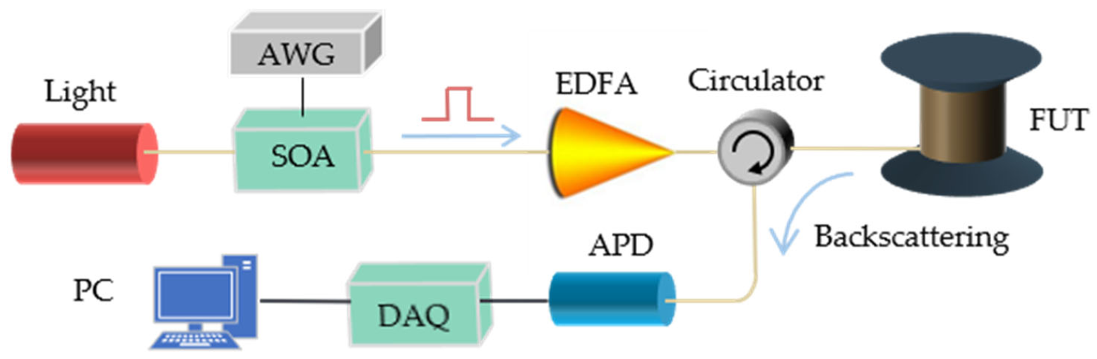
2.1. DVS
2.2. Data Collection
3. Deep CN
4. Results and Discussion
4.1. Training Process
4.2. Test Results
4.3. Comparison of Neural Networks
5. Conclusions, Limitations, and Future Research Trends
Author Contributions
Funding
Institutional Review Board Statement
Informed Consent Statement
Data Availability Statement
Conflicts of Interest
References
- Liu, K.; Sun, Z.; Jiang, J.; Ma, P.; Wang, S.; Weng, L.; Xu, Z.; Liu, T. A Combined events recognition scheme using hybrid features in distributed optical fiber vibration sensing system. IEEE Access 2019, 7, 105609–105616. [Google Scholar] [CrossRef]
- Li, J.; Wang, Y.; Wang, P.; Bai, Q.; Gao, Y.; Zhang, H.; Jin, B. Pattern recognition for distributed optical fiber vibration sensing: A review. IEEE Sens. J. 2021, 21, 11983–11998. [Google Scholar] [CrossRef]
- Yu, Z.; Zhang, Q.; Zhang, M.; Dai, H.; Zhang, J.; Liu, L.; Zhang, L.; Jin, X.; Wang, G.; Qi, G. Distributed optical fiber vibration sensing using phase-generated carrier demodulation algorithm. Appl. Phys. B 2018, 124, 84. [Google Scholar] [CrossRef]
- Pan, C.; Liu, X.; Zhu, H.; Shan, X.; Sun, X. Distributed optical fiber vibration sensor based on sagnac interference in conjunction with OTDR. Opt. Express 2015, 25, 20056–20070. [Google Scholar] [CrossRef] [PubMed]
- Zhu, H.; Pan, C.; Sun, X.; Ecke, W.; Peters, K.J.; Meyendorf, N.G. Vibration pattern recognition and classification in OTDR based distributed optical-fiber vibration sensing system. In Proceedings of the International Society for Optical Engineering, San Diego, CA, USA, 8 March 2014; p. 906205. [Google Scholar]
- Liu, K.; Tian, M.; Liu, Y.; Jiang, J.; Ding, Z.; Chen, Q.; Ma, C.; He, C.; Hu, H.; Zhang, X. A High-efficiency multiple events discrimination method in optical fiber perimeter security system. J. Lightwave Technol. 2015, 33, 4885–4890. [Google Scholar]
- Milne, D.; Masoudi, A.; Ferro, E.; Watson, G.; Pen, L. An analysis of railway track behaviour based on distributed optical fibre acoustic sensing. Mech. Syst. Signal Process. 2020, 142, 106769. [Google Scholar] [CrossRef]
- Wu, H.; Qian, Y.; Zhang, W.; Tang, C. Feature extraction and identification in distributed optical-fiber vibration sensing system for oil pipeline safety monitoring. Photonic Sens. 2017, 7, 305–310. [Google Scholar] [CrossRef] [Green Version]
- Rena, L.; Jiang, T.; Jia, Z.; Li, D.; Yuan, C.; Li, H. Pipeline corrosion and leakage monitoring based on the distributed optical fiber sensing technology. Measurement 2018, 122, 57–65. [Google Scholar] [CrossRef]
- Miah, K.; Potter, D. A review of hybrid fiber-optic distributed simultaneous vibration and temperature sensing technology and its geophysical applications. Sensors 2017, 17, 2511. [Google Scholar] [CrossRef] [PubMed] [Green Version]
- Jiang, F.; Li, H.; Zhang, Z.; Zhang, X.; Zhang, X.; Xiao, H.; Arregui, F.J.; Dong, L. An event recognition method for fiber distributed acoustic sensing systems based on the combination of MFCC and CNN. In Proceedings of the 2017 International Conference on Optical Instruments and Technology, Beijing, China, 10 January 2018; p. 1061804. [Google Scholar]
- Chao, T.; Ting, H. Research on pattern recognition technology of vibration signal form optical fiber sensing system. Opt. Commun. Technol. 2014, 38, 57–59. [Google Scholar]
- Lv, Y.; Wang, P.; Wang, Y.; Liu, X.; Bai, Q.; Li, P.; Zhang, H.; Gao, Y.; Jin, B. Eliminating phase drift for distributed optical fiber acoustic sensing system with empirical mode decomposition. Sensors 2019, 19, 5392. [Google Scholar] [CrossRef] [PubMed] [Green Version]
- Wu, Z.; Huang, N.E. Ensemble empirical mode decomposition: A noise-assisted data analysis method. Adv. Adapt. Data Anal. 2009, 1, 1–41. [Google Scholar] [CrossRef]
- Zhou, D.; Qin, Z.; Li, W.; Chen, L.; Bao, X. Distributed vibration sensing with time-resolved optical frequency-domain reflectometry. Opt. Express 2012, 20, 13138–13145. [Google Scholar] [CrossRef] [PubMed]
- Turner, C.; Joseph, A. A Wavelet packet and mel-frequency cepstral coefficients-based feature extraction method for speaker identification. Procedia Comput. Sci. 2015, 416–421. [Google Scholar] [CrossRef] [Green Version]
- Amin, H.U.; Malik, A.S.; Ahmad, R.F.; Badruddin, N.; Kamel, N.; Hussain, M.; Chooi, W. Feature extraction and classification for EEG signals using wavelet transform and machine learning techniques. Phys. Eng. Sci. Med. 2015, 38, 139–149. [Google Scholar] [CrossRef] [PubMed]
- Xu, C.; Guan, J.; Bao, M.; Lu, J.; Ye, W. Pattern recognition based on time-frequency analysis and convolutional neural networks for vibrational events in φ-OTDR. Opt. Eng. 2018, 57, 016103. [Google Scholar] [CrossRef]
- Wu, J.; Guan, L.; Bao, M.; Xu, Y.; Ye, W. Vibration events recognition of optical fiber based on multi-scale 1-D CNN. Opto-Electron. Eng. 2019, 46, 79–86. [Google Scholar]
- Li, S.; Peng, R.; Liu, Z. A surveillance system for urban buried pipeline subject to third-party threats based on fiber optic sensing and convolutional neural network. Struct. Health Monit. 2020, 20, 1704–1715. [Google Scholar] [CrossRef]
- Taylor, H.F.; Lee, C.E. Apparatus and Method for Fiber Optic Intrusion Sensing. U.S. Patent No. 5,194,847, 16 March 1993. [Google Scholar]
- Wang, F.; Xing, J. The influence of soil temperature on vibration signal in the optical fiber warning system. Opt. Tech. 2016, 42, 420–423. [Google Scholar]
- Eldan, R.; Shamir, O. The power of depth for feedforward neural networks. In Proceedings of the 29th Annual Conference on Learning Theory, New York, NY, USA, 23–26 June 2016; pp. 907–940. [Google Scholar]
- He, K.; Zhang, X.; Ren, S.; Sun, J. Deep residual learning for image recognition. In Proceedings of the IEEE Conference on Computer Vision and Pattern Recognition, Las Vegas, NV, USA, 27–30 June 2016; pp. 770–778. [Google Scholar]


| Class | Identify Category/% | Recognition Rate/% | ||
|---|---|---|---|---|
| Hammer | Air Pick | Excavator | ||
| Time–space domain + 2D CNN | 99.70 | 100 | 100 | 99.90 |
| Time-domain + 1D CNN | 97.59 | 99.44 | 97.77 | 98.28 |
| Frequency-domain + 1D CNN | 94.44 | 97.26 | 94.74 | 95.52 |
| Time–frequency domain + 2D CNN | 96.61 | 99.47 | 96.26 | 97.52 |
| Class | Identify Category/% | Recognition Rate/% | ||
|---|---|---|---|---|
| Hammer | Air Pick | Excavator | ||
| Time–space domain + 2D CNN | 97.76 | 99.70 | 100 | 99.20 |
| Time–domain + 1D CNN | 93.66 | 94.85 | 98.56 | 95.65 |
| Frequency-domain + 1D CNN | 97.76 | 85.45 | 97.47 | 93.03 |
| Time–frequency domain + 2D CNN | 97.76 | 93.03 | 96.39 | 95.54 |
| Class | Recognition Rate of Testset1 | Recognition Rate of Testset2 |
|---|---|---|
| Our CNN | 99.90% | 99.20% |
| CNN [20] | 98.76% | 65.83% |
Publisher’s Note: MDPI stays neutral with regard to jurisdictional claims in published maps and institutional affiliations. |
© 2022 by the authors. Licensee MDPI, Basel, Switzerland. This article is an open access article distributed under the terms and conditions of the Creative Commons Attribution (CC BY) license (https://creativecommons.org/licenses/by/4.0/).
Share and Cite
Ge, Z.; Wu, H.; Zhao, C.; Tang, M. High-Accuracy Event Classification of Distributed Optical Fiber Vibration Sensing Based on Time–Space Analysis. Sensors 2022, 22, 2053. https://doi.org/10.3390/s22052053
Ge Z, Wu H, Zhao C, Tang M. High-Accuracy Event Classification of Distributed Optical Fiber Vibration Sensing Based on Time–Space Analysis. Sensors. 2022; 22(5):2053. https://doi.org/10.3390/s22052053
Chicago/Turabian StyleGe, Zhao, Hao Wu, Can Zhao, and Ming Tang. 2022. "High-Accuracy Event Classification of Distributed Optical Fiber Vibration Sensing Based on Time–Space Analysis" Sensors 22, no. 5: 2053. https://doi.org/10.3390/s22052053