1. Introduction
An inertial measurement unit (IMU) aided by global navigation satellite system (GNSS) information is often used to track the six degree of freedom (DOF) pose (here, pose refers to the six degree of freedom position (x, y, z) and orientation (, , ) of the platform) of a moving platform. Solutions come in many forms but are broadly categorised as being tightly or loosely coupled depending on the level of sensor integration. The rationale for using the two sensor types is that GNSS receivers provide low-frequency information while the IMU provides information about higher frequency motion, noting that when stationary, the IMU measures gravity which can be considered as zero-frequency (DC) information. In a typical implementation, measurements from the two sensors are combined using optimal estimation methods, vis-à-vis Kalman filtering, to maintain an estimate of the pose of the platform frame P as it moves relative to a global frame G.
Where three GNSS receivers with non-collinear antenna are used, the low-frequency pose of the platform can be fully determined to the precision and bandwidth of the receivers. Each GNSS receiver provides positional knowledge of its antenna centres to a precision of approximately at a bandwidth from 0 to 2–5 (with measurement updates typically provided at 10 ). Higher frequency motion is then determined from information provided by the IMU, which will typically provide acceleration and angular rate information from 0 Hz to 50 Hz, at update rates of 50 Hz to 100 Hz. Such an arrangement provides a nice division of labour, with the Kalman filter-based pose estimator serving to combine the disparate frequency information provided by the two sensor types.
However, where two GNSS receivers are used, only five of the six degrees of freedom of the platform can be established using the information provided by the GNSS receivers. The platform’s rotational orientation about the line drawn through the antenna centres is not defined. In theory, gravity can be used to resolve this, provided the placement of the IMU frame does not result in the vector emanating from the sensor origin and directed by gravity, intersecting the antenna centre line. In practice, however, for a similarly structured estimator, start-up bias and the conflation of gravity measurement with accelerations due to platform motion limits the accuracy of pose estimates.
This paper develops and evaluates a method for using three-dimensional LiDAR measurements to stabilise pose estimates for platforms having two GNSS receivers. We consider two situations: (i) where the environment around the platform is a priori known, and (ii) where it is not. LiDAR sensors are often present on robotic platforms as components of a perception system. Their use for stabilising pose estimates becomes relevant where three GNSS receivers are impractical or cost-prohibitive.
Pose estimation is clearly ground for fertile research and has been for some time. Google Scholar identifies no fewer than 4650 publications that contain all of the terms “GNSS”, “IMU”, and “loosely coupled”. A total of 851 of these were published after 2020; the first was published in 1968 [
1]. If the term “pose” is included, 1050 papers are identified; 279 of these were published after 2020, while the earliest is [
2]. Adding the term “LiDAR” reduces the set to 452, of which 167 have been published since 2020, with the earliest again dating from 1981 [
3]. These, and the many other papers that use alternative but equivalent terminology, span a variety of approaches and applications, from terrestrial [
4,
5,
6], to aeronautical [
7,
8,
9,
10,
11], space [
12,
13,
14,
15]. In some instances, the search terms appear in reference to the technology being used for a specific application, e.g., precision agriculture [
16,
17,
18,
19] and construction [
20,
21]. In others, reference is made to implementation and algorithms. These are described at various levels of detail, but often with ambiguity.
Methods for stabilising pose estimates with LiDAR measurements exist and generally fall into two categories. The first are
feature-based methods which seek to identify features, sometimes known as landmarks, in LiDAR point clouds and maintain an estimate of their location. Features can be lines or planes [
22,
23,
24], curves [
25,
26], or corners [
27]. Feature-based methods can also match sequential LiDAR scans, solving for the incremental change in pose between scans [
28,
29,
30,
31,
32].
An alternative approach uses model-based methods. These generally compare measurements from a ranging sensor with a model of the environment, searching for a pose solution that provides an optimal solution.
Ref. [
33] propose an airborne solution for aiding a navigation system through the use of a large-scale terrain model and LiDAR sensors. Similarly, Ref. [
34] augment pose estimates by fitting LiDAR measurements against a known two-dimensional environment model. Refs. [
35,
36] show how pose estimates of known objects can be obtained from only LiDAR scans by finding the pose that is most likely among the set of all possible poses.
Other work has focused on the augmentation of pose when GNSS measurements are degraded or unavailable, such as loss of real-time kinematic (RTK) corrections. Ref. [
37] develop a solution that uses a known geometric model of the world and that augments GNSS measurements with a pseudo-measurement of the expected height of the receiver. Ref. [
38] use a conceptually similar approach, but apply it to aerial vehicles.
Work on
model-based methods has also focused on building an environment model simultaneously with localisation within this model. One solution, presented by [
39], develops an algorithm for a LiDAR- and GNSS-aided IMU navigation system for use in an airborne platform that only maps the terrain when GNSS and IMU measurements are available and reliable. When the integrity of the GNSS-aided IMU navigation system is compromised, LiDAR observations are fitted to the generated terrain model through an ICP-based method. The authors find that the solution is robust and improves the accuracy of the pose when the GNSS system is in a degraded state.
Ref. [
40] present a method that augments a GNSS-aided IMU and odometry navigation system with a scanning LiDAR sensor. The authors estimate the environment using the LiDAR scanner as they move through an urban scene, and remove dynamic obstacles by compressing this model to a ground plane, coloured based on infrared reflectivity from LiDAR return intensities. They identify that their novel navigation system is up to an order of magnitude more accurate than a GNSS-aided IMU and odometry navigation system.
Our rationale for writing this paper is twofold. First, we believe the approach we propose for the integration of LiDAR measurement into a GNSS-aided IMU solution is novel. Second, we have repeatedly sought clear descriptions of the algorithms others have used, only to find missing details or gaps that have frustrated our implementation efforts. Here, we attempt to give a full and complete description of a loosely coupled GNSS-aided IMU navigation system in the expectation that it will be useful to others.
2. Experimental Platform
Figure 1 shows the experimental platform considered in this paper. The machine is called a track-type tractor or bulldozer and has applications in agriculture, construction, and mining. In all these domains, tracking spatial pose is needed for technology applications that include production reporting, guidance, and automation.
Figure 1 shows the coordinate frames in which variables relevant to the development of the pose estimation system are represented. The global frame is denoted as
G. Frame
P describes the pose of the tractor in Frame
G by a transformation
. Sensors are described relative to Frame
P: Frame
I describes the position and orientation of the IMU; Frame
L describes the position and orientation of a LiDAR; and
and
are the centres of the antennas of two GNSS receivers mounted on the tractor cabin.
The pose of the tractor is defined by the state vector,
The 21 state parameters of the state vector are intended to accommodate a constant acceleration model for translation and a constant rate model for attitude. Here,
is the coordinate of the origin of P in G;
is the velocity of point in G;
is the acceleration of point in G;
describes the attitude of Frame P in G as , and ;
describes the rotational velocity of Frame P in G;
describes the acceleration bias of the IMU in Frame I;
is the rotational rate bias of the IMU in Frame I.
The transformation matrix
is given by
where
Here, is the cosine function and is the sine function. Note, transforms points in Frame P into Frame G; equally, it describes the location of Frame P in Frame G. The top left block of the matrix is the rotation matrix which aligns Frame P in Frame G.
The IMU provides measurements at 50
; the GNSS receivers are RTK-enabled and provide observations at 10
. The LiDAR is a Velodyne VLP-16 and provides range measurements from 16 beams, equally spaced across a field of view of 30
with 360
and rotation at 10
. Other details of the sensors are given in
Table 1.
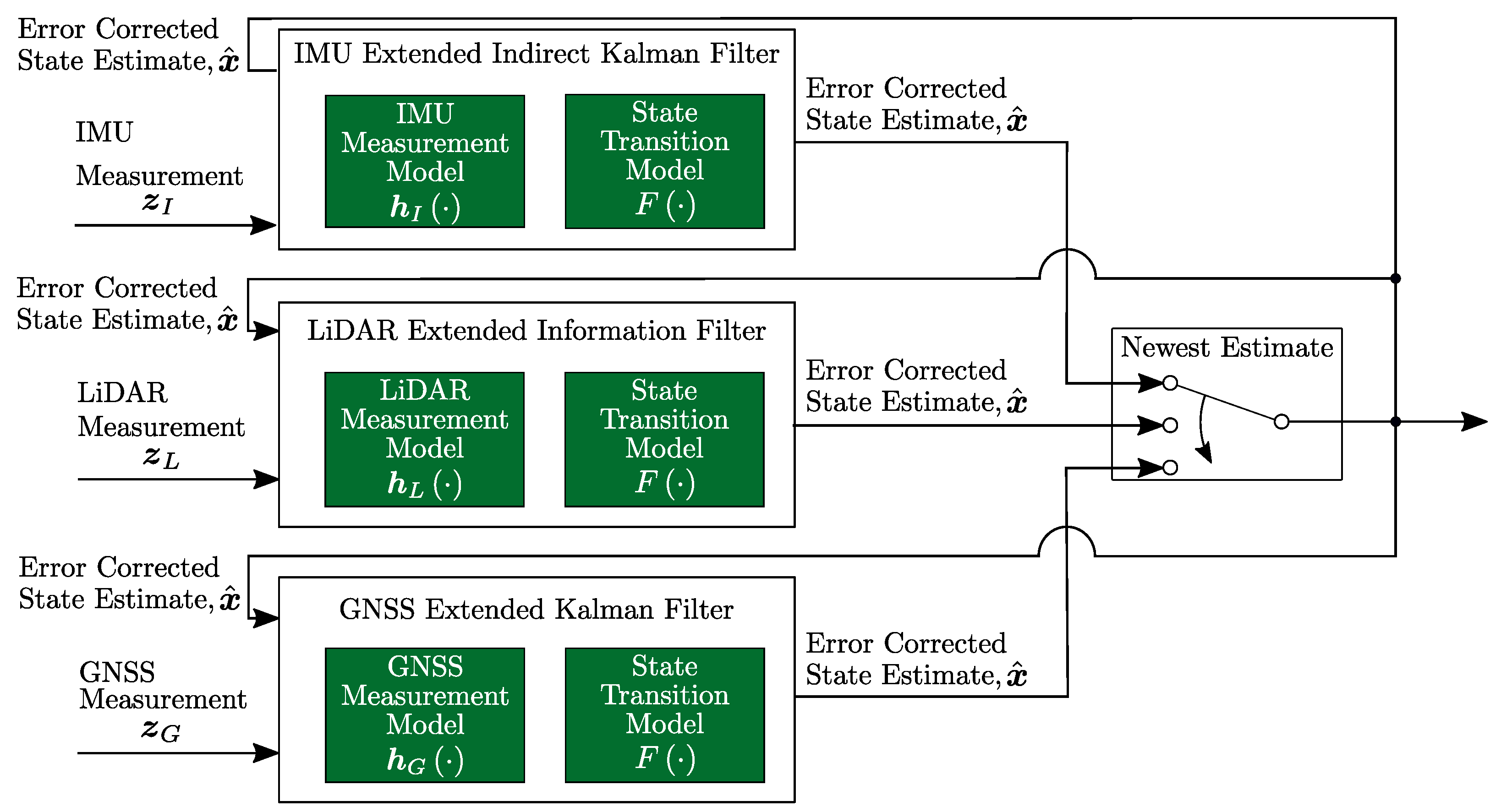
4. Process Model
The three filter updates of
Figure 2 share the same process model which is assumed linear having the discrete-time form
The state transition model
predicts the platform’s state vector assuming a constant acceleration for translations and a constant rate for rotations. The state transition model also predicts the IMU acceleration and rotational rate biases through use of constants determined from experimental observations (see [
51]). The
matrix
has the form
Here,
describes the empirically determined accelerometer bias parameters, and
the empirically determined gyroscope bias parameters. Observe that
The second term of the right-hand side of Equation (
4) describes the process noise which accounts for modelling approximations and model integration errors. We define
where
is a white Gaussian discrete-time process and
is Brownian motion with diffusion
such that for consecutive measurement times
and
,
If the sample period is assumed to be small compared to the auto-correlation times of the process model modes,
Observe that if the diffusion is time-invariant, the process noise covariance, , increases linearly from the time since the last measurement. As this time increases, the process noise increases, resulting in the process model being weighted less in the Kalman filter update and measurements being weighted more.
8. Evaluation
It is necessary to use indirect methods for the evaluation of the pose estimator as there no is ground truth pose trajectory. The approach chosen is to survey the environment to obtain a ground truth model and compare LiDAR measurements with the predicted ranges from ray-casting against this scanned ground truth model. These differences are representative of the error in the pose. The survey to obtain the ground truth model was created with a Faro Focus
3D terrestrial LiDAR scanner [
54]. This instrument claims a one standard deviation range precision of
.
Figure 8 shows the environment model obtained by scanning.
The scene used for evaluation is shown in
Figure 9. It comprises a generally flat terrain with piled dirt, forming mounds. The bulldozer was manually moved around in this environment following the path shown in
Figure 8. During the execution of this motion, at various points, the platform was pitched and rolled using the bulldozer blade.
Figure 10 shows the point-to-model errors for the GNSS-aided IMU solution and the LiDAR- and GNSS-aided solution in a known environment. A ray having the length of the measurement is cast along the corresponding LiDAR beam at the estimated pose. The distance from the end point of the ray to the nearest point of the model is determined as the point-to-model error. The smaller the point-to-model error, the closer the real pose to the estimated pose. For perfect pose, a perfect model, and zero measurement error, the point-to-model error is zero.
The distribution of point-to-model errors given in
Figure 10 evidences that the LiDAR- and GNSS-aided IMU solution is more accurate than the GNSS aiding. The mean point-to-model error is reduced from
to
. Significantly, the highest number of point-to-model errors for the LiDAR- and GNSS-aided solution corresponds to zero error. This is not unexpected: the positioning of the GNSS antennas provides information that supports good spatial positioning along with roll and yaw estimation. However, no information is available from GNSS measurements about the orientation of the axis that passes through the two antenna centres. This rotation heavily contributes to the pitch of the platform. The provision of measurements of the forward-facing 3D LiDAR provides information that stabilises the pitch estimate, this accounting for the improved accuracy. The mean value for point-to-model error for the GNSS-aided solution is prospectively due to start-up bias on the centre. It is noted that the GNSS-aided solution has a broader distribution of error.
The time estimates for the six degrees of freedom of the platform’s pose are shown in
Figure 11. Significantly both estimators give similar results for
x,
y,
z, and yaw. Most of the difference is in estimates for the pitch and roll of the platform. The bias in the pitch estimate for the GNSS-aided solution is attributed to start-up bias in the IMU sensor, which the estimator has been unable to account for; it is present at both the start and end of the motion sequence when the platform is stationary.
The results in this paper were produced on a computer running a Linux-based operating system (Intel Xeon W-2125 CPU, 32 GB of memory). The GNSS-aided IMU filter could update up to ∼ , much faster than the measurement rate. The LiDAR- and GNSS-aided IMU filter required more computing per time step and was capable of ∼ 500 .
9. LiDAR Measurement Model in an Unknown Environment
The capability to estimate pose when the environment is known helps to establish the potential performance of the LiDAR- and GNSS-aiding estimator, but is of limited practical usefulness. Most environments of interest in which this platform operates have unknown geometry. The estimator is extended to achieve the benefits of pitch stabilisation provided by the LiDAR measurement by concurrently estimating the pose and the local terrain.
For this purpose, the terrain is modelled as a height grid that divides the
plane into a regular grid. Each grid element, known as a cell, is assigned a height. The points defined by each cell in the height grid can be triangulated to develop a representation of the terrain as a surface. A representation of the triangulated height grid with states
to
is shown in
Figure 12.
Each of the
cell heights in the grid can be considered additional states for which estimates are sought. These states, collectively denoted
, augment the state vector defined by Equation (
1), shown here as
. Here,
takes the form
The subscript
t indicates terrain. The additional terrain state estimates are appended to the state vector as follows:
As the terrain model is now part of the state vector, the LiDAR observation function is of the form
The measurement function used to estimate the terrain and pose is identical to that of the previous section. However, expected range measurements are now determined through ray-casting onto the triangulated height grid model constructed from the vector, not a provided static model. The z-value or height of the vertices of each triangle of the grid, , and , are now defined by the elements of . The measurement Jacobian for the terrain states is determined analytically from the partial derivative of the LiDAR range measurement with respect to the z-value of the points of the intercepted triangle (, and ).
Figure 13 shows that the concurrent terrain and pose estimation system performs slightly worse than the LiDAR- and GNSS-aided IMU solution and significantly better than the GNSS-aided IMU solution. The mean point-to-model error for the concurrent terrain and pose estimation system is
. The zero point-to-model error bin is the largest bin, with the error distribution extending to higher point-to-model error values.
Figure 14 shows the environment model generated by the concurrent terrain and pose estimation system. The terrain model is coloured based on the difference between the estimated terrain and the surveyed ground truth model. The terrain estimate shows close agreement with the truth model: generally, state errors are less than
but extend out to
. The terrain estimate has an RMS error of
, which was achieved using a 1
height grid terrain representation. Generally, areas of large error are present in high gradient locations of the terrain model. These can be difficult to capture using a regular grid terrain representation.
The estimates of the six degrees of freedom of the platform’s pose are shown in
Figure 15. The solution generated without
a priori knowledge of this environment shows some deviation in both roll and pitch when compared to that obtained using a known environment. The forward-looking orientation of the LiDAR sensor clearly stabilises the pitch estimate; the roll estimate is similar to the GNSS-aided IMU solution. A wider three-dimensional scan is expected to yield better stabilisation of roll. Equally, better roll estimates could be achieved by increasing the space between the GNSS antennas. The yaw,
x,
y, and
z degrees of freedom are similar to those estimated when the environment is known. Overall, the results demonstrate the effectiveness of the approach.
The concurrent terrain and pose estimation filter, again, required more computing per timestep. It was demonstrated to run at ∼ 50
on the target hardware (see
Section 8).
10. Conclusions
The main result from this work is to show how LiDAR can be used to stabilise two-antenna GNSS-aided IMU pose estimators in environments with known and unknown geometry. The formulation is structured to accommodate multi-rate and non-synchronous measurements. It enables continuity through short-term periods of lost measurements from one of the sensors. Lost measurements are a characteristic observed on some brands of RTK-GNSS receivers, and the solution described in this paper adapts well to this situation.
We have not explored the possibility of using LiDAR stabilisation in GNSS-denied environments; however, the approach described here could be readily adapted to such situations.
In the paper introduction, we identified that LiDAR- and GNSS-aided IMU solutions can be effective when three-dimensional LiDAR measurements are available, but that three GNSS receivers are impractical or cost-prohibitive. Our recommendation, based on experience, is that if three receivers are possible, they should be used, particularly if an accurate pose solution to high frequencies is required.


