
Infrared Visual Sensing Detection of Groove Width for Swing Arc Narrow Gap Welding


Abstract
:1. Introduction
2. Infrared Passive Visual Sensing Detection System for Groove Width
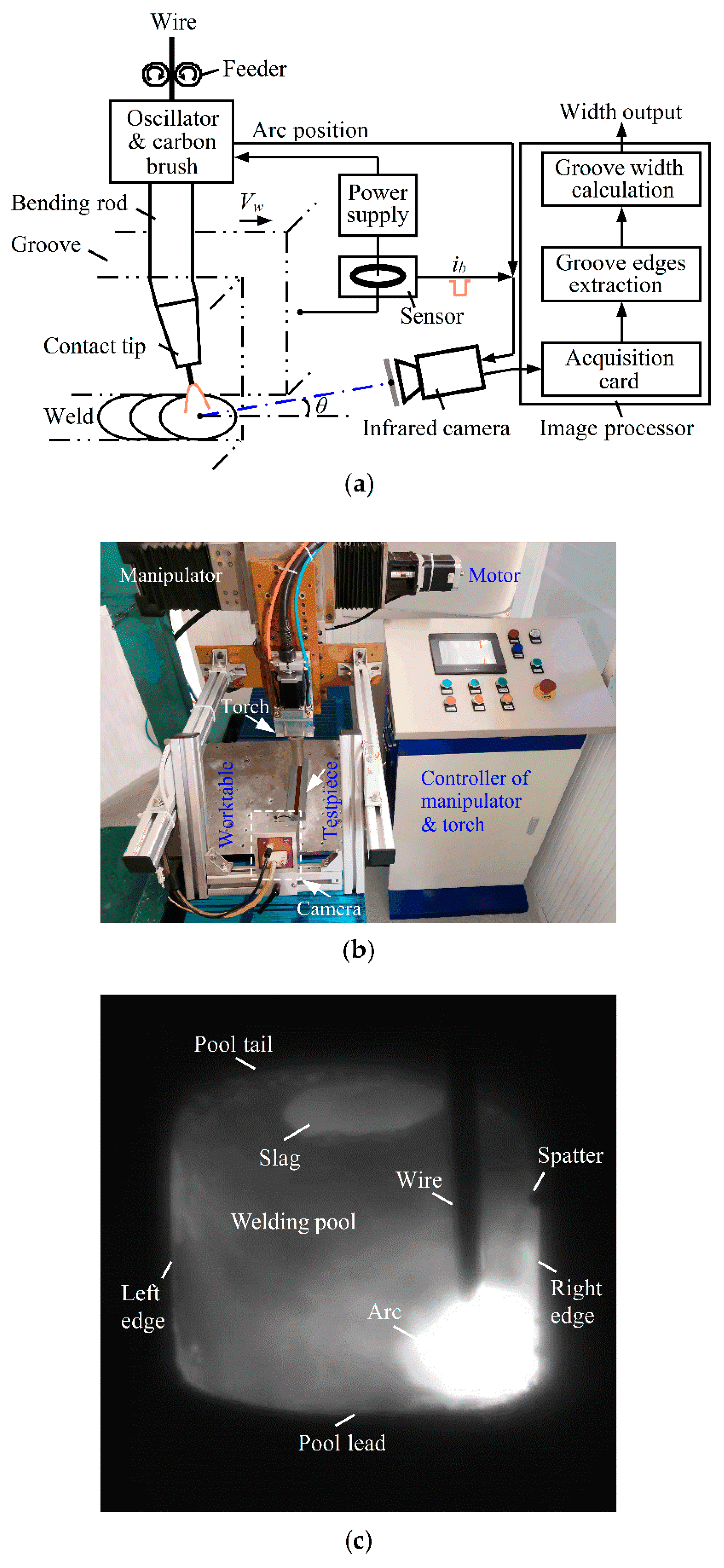
2.1. System Construction
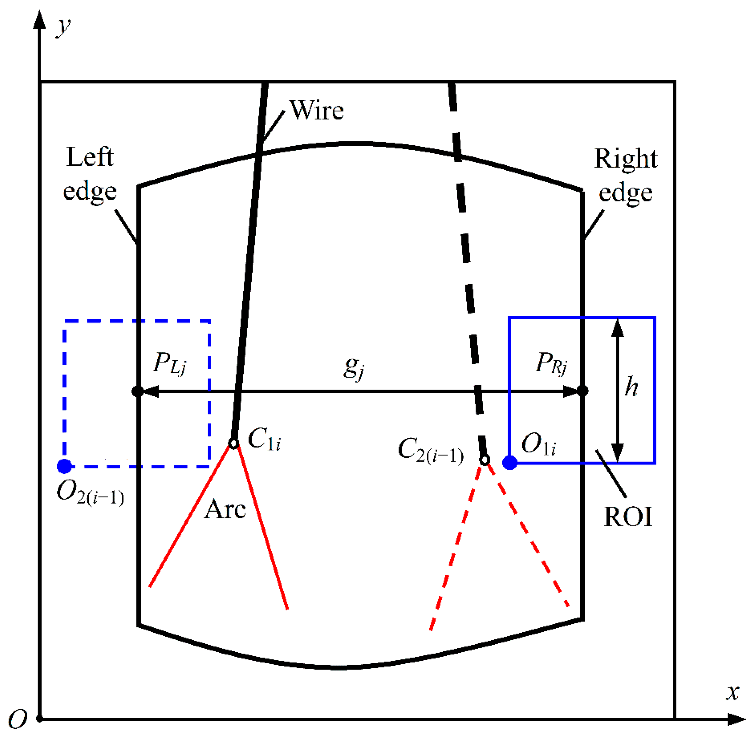
2.2. Detection Principle
3. Division Thresholding Method of ROI Window Image
4. In Situ Dynamic Clustering Algorithm
4.1. Principle of ISDC Algorithm
4.1.1. Data Preprocessing
4.1.2. Dynamic Clustering
Determination of Initial Cluster Center
Dynamic Clustering
Renewal of Cluster Center
4.1.3. Cluster Selection
4.2. Dynamic Analysis of ISDC Algorithm
4.3. Adaptability of ISDC Algorithm
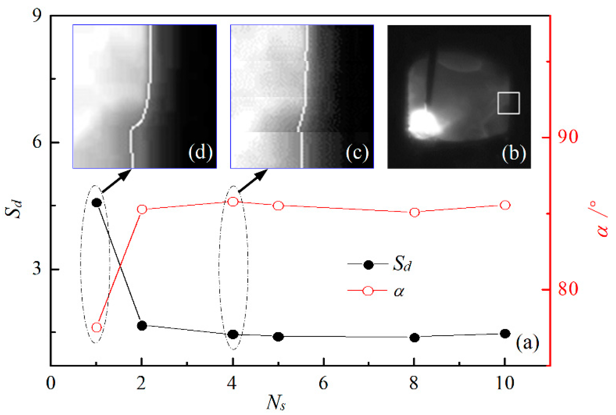
4.3.1. Effect of Cluster Selection Threshold
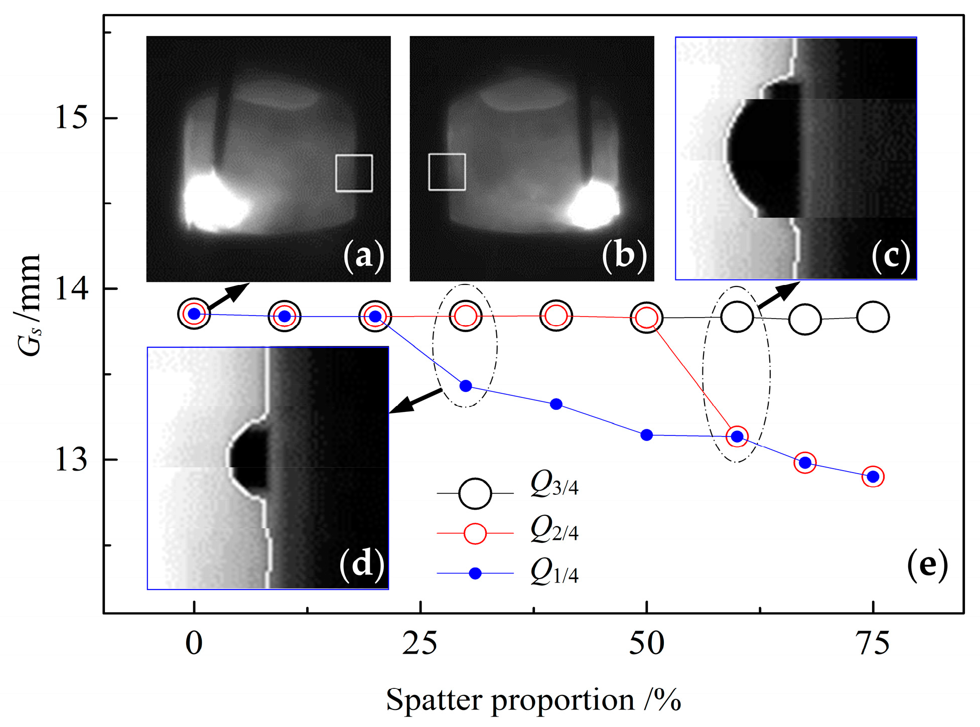
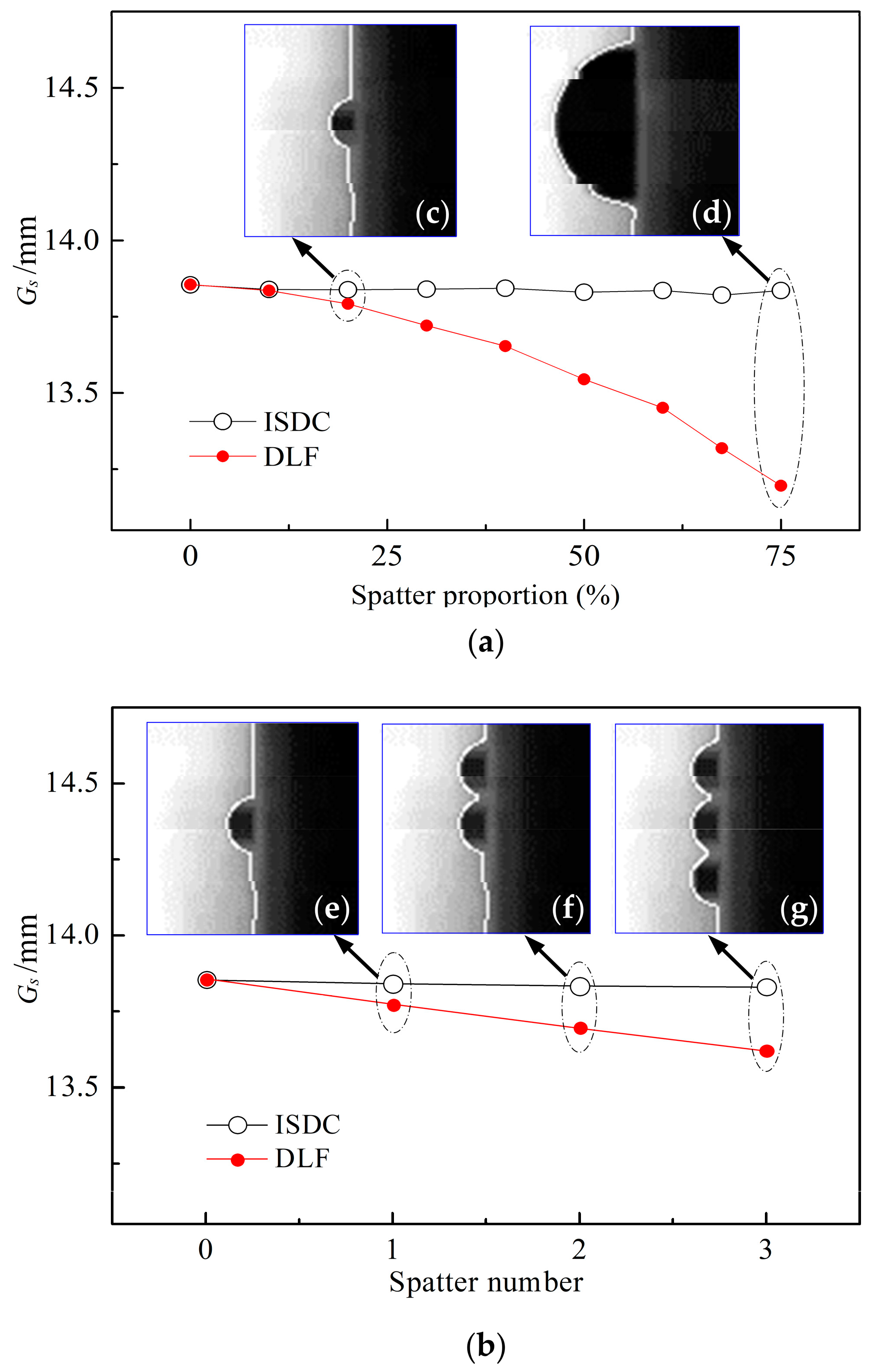
4.3.2. Effect of Welding Spatter
5. Experimental Results of Groove Width Detection
5.1. Experimental Welding Conditions
5.2. Experimental Results for Constant-Width Groove
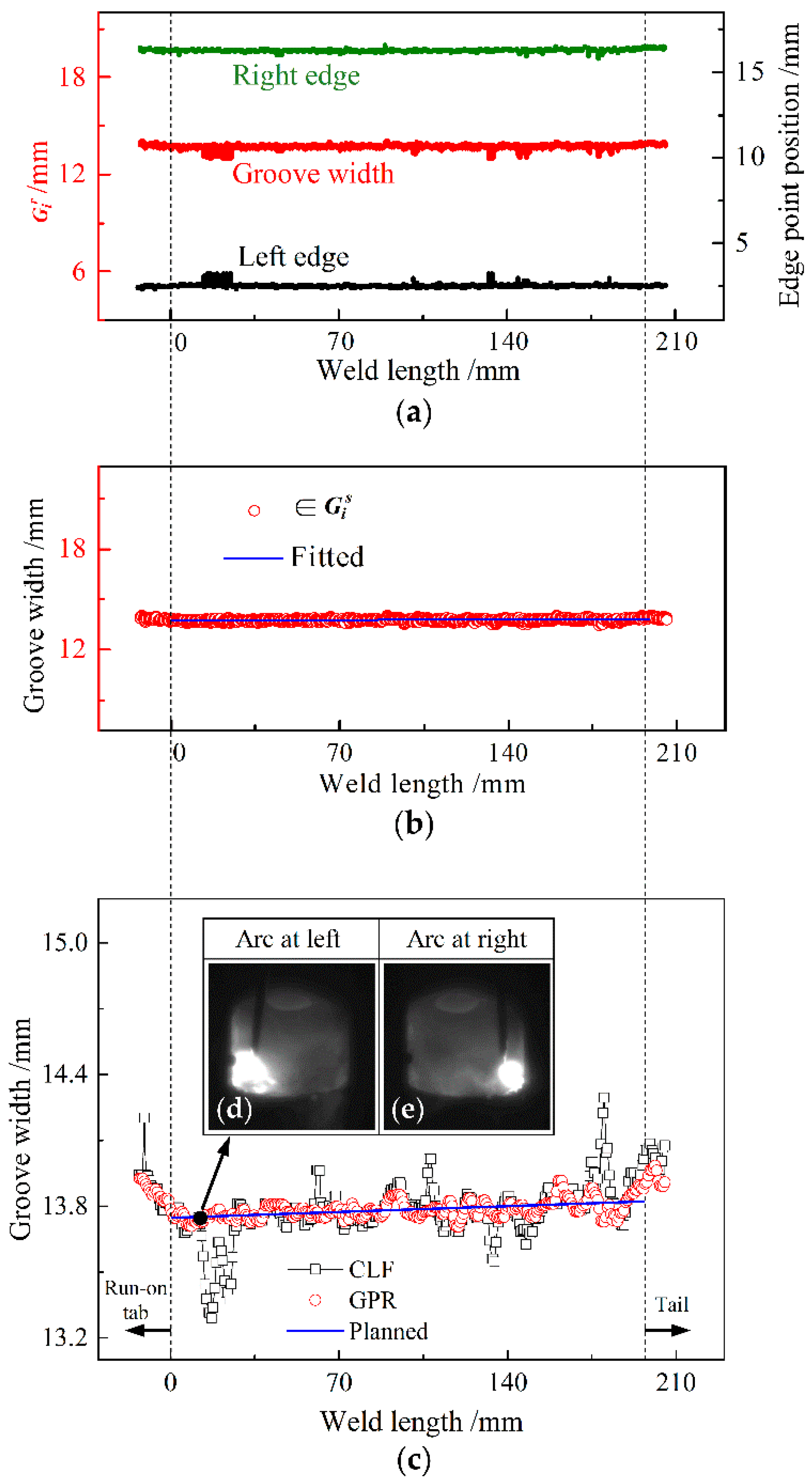
5.3. Experimental Results for Width-Varying Groove
5.4. Weld Formation Analysis
6. Conclusions
Author Contributions
Funding
Institutional Review Board Statement
Informed Consent Statement
Data Availability Statement
Conflicts of Interest
References
- Malin, V. The state-of-the-art of narrow gap welding. Weld. J. 1983, 62, 22–30. [Google Scholar]
- Kang, Y.H.; Na, S.J. Characteristics of welding and arc signal in narrow groove gas metal arc welding using electromagnetic arc oscillation. Weld. J. 2003, 5, 93–99. [Google Scholar]
- Ribeiro, R.; Assunção, P.; Dos Santos, E.; Filho, A.; Braga, E.; Gerlich, A. Application of cold wire gas metal arc welding for narrow gap welding (NGW) of high strength low alloy steel. Materials 2019, 12, 335. [Google Scholar] [CrossRef] [PubMed] [Green Version]
- Liu, G.Q.; Tang, X.H.; Xu, Q.; Lu, F.G.; Cui, H.C. Effects of active gases on droplet transfer and weld morphology in pulsed-current NG-GMAW of mild steel. Chin. J. Mech. Eng. 2021, 34, 66. [Google Scholar] [CrossRef]
- Sugitani, Y.; Kobayashi, Y.; Murayama, M. Development and application of automatic high speed rotation arc welding. Weld. Int. 1991, 5, 577–583. [Google Scholar] [CrossRef]
- Iwata, S.; Murayama, M.; Kojima, Y. Application of narrow gap welding process with high speed rotating arc to box column joints of heavy thick plates. JFE Technol. Rep. 2009, 14, 16–21. [Google Scholar]
- Mortvedt, D.H. Evaluation of the usability and benefits of twist wire GMAW and FCAW narrow gap welding. J. Ship Prod. Des. 1986, 2, 23–33. [Google Scholar] [CrossRef]
- Murayama, M.; Oazamoto, D.; Ooe, K. Narrow gap gas metal arc (GMA) welding technologies. JFE Technol. Rep. 2015, 20, 147–153. [Google Scholar]
- Wang, J.Y.; Ren, Y.S.; Yang, F.; Guo, H.B. Novel rotation arc system for narrow gap MAG welding. Sci. Technol. Weld. Join. 2007, 12, 505–507. [Google Scholar] [CrossRef]
- Wang, J.Y.; Zhu, J.; Fu, P.; Su, R.J.; Han, W.; Yang, F. A swing arc system for narrow gap GMA welding. ISIJ Int. 2012, 52, 110–114. [Google Scholar] [CrossRef] [Green Version]
- Wang, J.Y.; Zhu, J.; Zhang, C.; Wang, N.; Su, R.J.; Yang, F. Development of swing arc narrow gap vertical welding process. ISIJ Int. 2015, 55, 1076–1082. [Google Scholar] [CrossRef] [Green Version]
- Wang, J.Y.; Zhu, J.; Zhang, C.; Xu, G.X.; Li, W.H. Effect of arc swing parameters on narrow gap vertical GMA weld formation. ISIJ Int. 2016, 56, 844–850. [Google Scholar] [CrossRef] [Green Version]
- Xu, G.X.; Wang, J.Y.; Li, P.; Zhu, J.; Cao, Q. Numerical analysis of heat transfer and fluid flow in swing arc narrow gap GMA welding. J. Mater. Process. Technol. 2018, 252, 260–269. [Google Scholar] [CrossRef]
- Xu, G.X.; Li, L.; Wang, J.Y.; Zhu, J.; Li, P. Study of weld formation in swing arc narrow gap vertical GMA welding by numerical modeling and experiment. Int. J. Adv. Manuf. Technol. 2018, 96, 1905–1917. [Google Scholar] [CrossRef]
- Fabry, C.; Pittner, A.; Rethmeier, M. Design of neural network arc sensor for gap width detection in automated narrow gap GMAW. Weld. World 2018, 62, 819–830. [Google Scholar] [CrossRef]
- Liu, W.J.; Guan, Z.Y.; Jiang, X.; Li, L.Y.; Yue, J.F. Research on the seam tracking of narrow gap P-GMAW based on arc sound sensing. Sensor. Actuat. A-Phys. 2019, 292, 205–216. [Google Scholar]
- Xue, B.C.; Chang, B.H.; Peng, G.D.; Gao, Y.J.; Tian, Z.J.; Du, D. A vision based detection method for narrow butt joints and a robotic seam tracking system. Sensors 2019, 19, 1144. [Google Scholar] [CrossRef] [Green Version]
- Yamazaki, Y.; Abe, Y.; Hioki, Y.; Nakatani, M.; Kitagawa, A.; Nakata, K. Development of gap sensing system for narrow gap laser welding. Weld. Int. 2016, 30, 745–754. [Google Scholar] [CrossRef]
- Zhu, J.; Wang, J.Y.; Su, N.; Xu, G.X.; Yang, M.S. An infrared visual sensing detection approach for swing arc narrow gap weld deviation. J. Mater. Process. Technol. 2017, 243, 258–268. [Google Scholar] [CrossRef]
- Zhang, B.R.; Shi, Y.H.; Gu, S.Y. Narrow-seam identification and deviation detection in keyhole deep-penetration TIG welding. Int. J. Adv. Manuf. Technol. 2018, 101, 2051–2064. [Google Scholar] [CrossRef]
- Li, W.H.; He, C.F.; Chang, J.S.; Wang, J.Y.; Wu, J. Modeling of weld formation in variable groove narrow gap welding by rotating GMAW. J. Manuf. Process. 2020, 57, 163–173. [Google Scholar] [CrossRef]
- Chen, Y.K.; Shi, Y.H.; Cui, Y.X.; Chen, X.Y. Narrow gap deviation detection in Keyhole TIG welding using image processing method based on Mask-RCNN model. Int. J. Adv. Manuf. Technol. 2021, 112, 2015–2025. [Google Scholar] [CrossRef]
- Pinto-Lopera, J.; Motta, J.; Alfaro, S. Real-time measurement of width and height of weld beads in GMAW processes. Sensors 2016, 16, 1500. [Google Scholar] [CrossRef] [PubMed]
- Comas, T.F.; Diao, C.L.; Ding, J.L.; Williams, S.; Zhao, Y.F. A passive imaging system for geometry measurement for the plasma arc welding process. IEEE Trans. Ind. Electron. 2017, 64, 7201–7209. [Google Scholar] [CrossRef] [Green Version]
- Hong, Y.X.; Chang, B.H.; Peng, G.D.; Zhang, Y.; Hou, X.C.; Xue, B.C.; Du, D. In-process monitoring of lack of fusion in ultra-thin sheets edge welding using machine vision. Sensors 2018, 14, 2411. [Google Scholar] [CrossRef] [Green Version]
- Shao, W.; Liu, X.; Wu, Z. A robust weld seam detection method based on particle filter for laser welding by using a passive vision sensor. Int. J. Adv. Manuf. Technol. 2019, 104, 2971–2980. [Google Scholar] [CrossRef]
- Yamane, S. Tracking the welding line in lap welding using pattern matching. ISIJ Int. 2020, 60, 1752–1757. [Google Scholar] [CrossRef]
- Xiong, J.; Liu, Y.; Yin, Z. Passive vision measurement for robust reconstruction of molten pool in wire and arc additive manufacturing. Measurement 2020, 153, 107407. [Google Scholar] [CrossRef]
- Chen, C.; Lv, N.; Chen, S.B. Welding penetration monitoring for pulsed GTAW using visual sensor based on AAM and random forests. J. Manuf. Process. 2021, 63, 152–162. [Google Scholar] [CrossRef]
- Jamrozik, W.; Górka, J. Assessing MMA welding process stability using machine vision-based arc features tracking system. Sensors 2020, 21, 84. [Google Scholar] [CrossRef]
- Yu, R.; Kershaw, J.; Wang, P.; Zhang, Y.M. Real-time recognition of arc weld pool using image segmentation network. J. Manuf. Process. 2021, 72, 159–167. [Google Scholar] [CrossRef]
- Gonzalez, R.C.; Woods, R.E. Digital Image Processing, 3rd ed.; Pearson Prentice Hall: Upper Saddle River, NJ, USA, 2008; pp. 627–787. [Google Scholar]


| Parameter Name | Value |
|---|---|
| Central wavelength of narrowband filter (nm) | 970 |
| Neutral density filter (%) | 30 |
| Aperture | f/16 |
| Exposure time (ms) | 0.3 |
| Shooting depression angle θ (°) | 20 |
| Global image size (pixels) | 544 × 544 |
| Parameter Name | Value |
|---|---|
| Average arc current (A) | 302.5 |
| Average arc voltage (V) | 28.7 |
| Arc current pulse frequency (Hz) | ~222 |
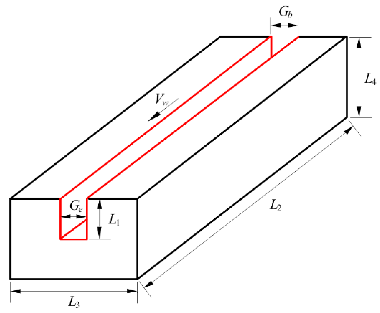
| Welding speed Vw (mm s−1) | 3.4 |
| Solid wire diameter (mm) | 1.2 |
| Torch standoff height (mm) | 20 |
| Shielding gas/flowrate (L min−1) | Ar−20% CO2/25 |
| Groove gap (mm) | 14 |
| Arc swing frequency (Hz) | 2.5 |
| Arc swing angle (°) | 82 |
| Arc at-sidewall staying time (s) | 0.1 |
| Conductive rod bending angle (°) | 8 |
| Algorithm | Standard Deviation of Groove Edge Point Distribution | Size of Resistible Spatter | Error Range of Width Detection | Standard Deviation of Width Detection |
|---|---|---|---|---|
| GPR | 1.449 | ≤2.19 mm | −0.086~+0.109 mm | 0.035 |
| CLF | 4.581 | ≤0.58 mm | −0.465~+0.479 mm | 0.115 |
| Algorithm | Error Range (mm) | Standard Deviation |
|---|---|---|
| GPR | −0.168~+0.119 | 0.058 |
| CLF | −0.447~+0.196 | 0.103 |
Publisher’s Note: MDPI stays neutral with regard to jurisdictional claims in published maps and institutional affiliations. |
© 2022 by the authors. Licensee MDPI, Basel, Switzerland. This article is an open access article distributed under the terms and conditions of the Creative Commons Attribution (CC BY) license (https://creativecommons.org/licenses/by/4.0/).
Share and Cite
Su, N.; Wang, J.; Xu, G.; Zhu, J.; Jiang, Y. Infrared Visual Sensing Detection of Groove Width for Swing Arc Narrow Gap Welding. Sensors 2022, 22, 2555. https://doi.org/10.3390/s22072555
Su N, Wang J, Xu G, Zhu J, Jiang Y. Infrared Visual Sensing Detection of Groove Width for Swing Arc Narrow Gap Welding. Sensors. 2022; 22(7):2555. https://doi.org/10.3390/s22072555
Chicago/Turabian StyleSu, Na, Jiayou Wang, Guoxiang Xu, Jie Zhu, and Yuqing Jiang. 2022. "Infrared Visual Sensing Detection of Groove Width for Swing Arc Narrow Gap Welding" Sensors 22, no. 7: 2555. https://doi.org/10.3390/s22072555