1. Introduction
Arterial hypotension that occurs during anesthesia may increase the incidence of postoperative complications, such as myocardial infarction or acute kidney injury [
1]. Careful monitoring of the patient’s hemodynamic changes is required during anesthesia, and when hypotension is detected, immediate treatment is provided to maintain hemodynamic stability. If the patient’s hemodynamic changes are predicted in advance, it will be possible to provide safer anesthesia to the patient by maintaining hemodynamic stability. Most patient monitor devices that monitor a patient’s vital signs store the data for a short time [
2], and the data are mostly deleted without being utilized for other purposes.
However, these vital sign data can be useful in developing a tool which can predict a patient’s hemodynamic changes.
While research on hypotension in operation room mostly focuses on investigating the factors affecting a hypotension event, not much research has been performed on real-time prediction of hypotension. The advanced warning that hypotension is imminent at least 5 min ahead enables clinicians to take proper measures to reduce the impact of hypotension. This forecasting problem is quite challenging compared to diagnosis that detects high-risk patients at current. The forecasting problem that does not specify when the event occurs is easier than the forecasting problem that specifies the event time. Furthermore, it is very difficult to advance the predictable time compared to the event occurrence time. In this work, we will challenge the forecasting problem in 5 min advance.
Previous works on hypotension prediction have proposed various indices that originate from the waveform of vital signs. Recently, machine learning algorithms have replaced the scoring system, identified significant factors, and measured their effect on an event automatically.
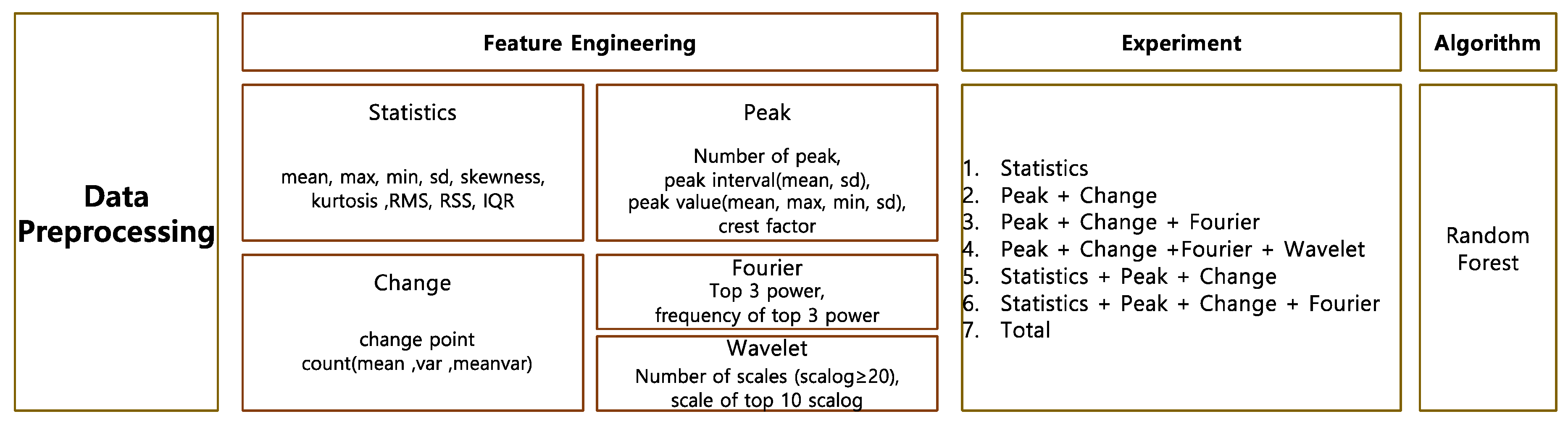
In this study, we propose a systematic feature engineering that is applicable to any kind of vital signs and build a machine learning model that predicts hypotension in advance. We aim to build a simple model that does not require many vital signs and only requires invasive blood pressure (IBP). Instead of hand-crafted features on IBP, we propose a common feature extraction model that can be applicable to various kinds of vital signs. The feature extraction model includes the statistical analysis, peak analysis, change analysis, and frequency analysis. We build an ensemble model using a random forest model to handle numerous features in heterogenous samples.
2. Related Works
Many studies using vital signs have been performed in the intensive care unit (ICU); however, there is little research for the operation room where vitality is relatively constant compared to ICU [
3,
4,
5,
6,
7,
8,
9].
Recently, studies that predict hypotension, depth of anesthesia, hypothermia, etc., have been conducted in the operating room. Topics of the studies using vital signals during surgery encompass estimation of the depth of anesthesia, estimation of blood pressure, event prediction regarding blood pressure, and heart failure. The former models were designed to predict whether a patient would suffer an event or not at the initial stage of operation [
10,
11,
12,
13,
14]. These works can inform high-risk patients, but are limited in alerting an alarm for real-time treatment for an event. The recent prediction models are developed into real-time prediction models and the number of works is limited. We briefly reviewed real-time models in terms of classification and regression.
2.1. Real-Time Event Detection
Yang et al. [
15] reported a convolutional neural network (CNN)-based deep learning model that predicts the stroke volume with a 20 s arterial blood pressure waveform. Lee et al. [
16] created a CNN-based deep learning model to predict hypotension before 5 min, 10 min, and 15 min, respectively, using IBP, electrocardiography (ECG), photoplethysmography (PPG), and capnography (CO
2). They demonstrated that the precision and recall were higher than our research, but their experimental setting was different from ours. They included only the period where non-hypotension lasted for 20 min only. Their environment was less realistic because their model did not work on samples that included any data below the criteria. In addition, it is not sure that they focused on predictions for the very first time point of hypotension. As hypotension occurred, an alarm given in a timely manner was required in the first place. Chen and Qi [
17] proposed a feature-based model. They predicted heart failure by statistical features; textualization; and imaging using HR, SBP, DBP, SpO
2, and pulse pressure difference (PP). Among the statistical feature models, the gradient boosting tree model had the highest accuracy of 84%, while textualization and imaging models had accuracies of 81% and 83% for the logistic regression and convolution neural network models, respectively. Furthermore, in predicting heart failure, the statistical feature-based model gave the best results. The statistical features used in this study included the mean; variance; minimum; maximum; 25%, 50%, and 75% quantiles; skewness; kurtosis; and first-order difference of each feature.
These real-time detection models suffer from the class imbalance problem and rarely achieve good performance. Most works set up an artificial environment to make the models work.
2.2. Real-Time Regression
The following works have been proposed to real-time regression for blood pressure or depth of anesthesia. The real-time regression model showed better performance compared to the event detection model because regression models are free from the class imbalance problem that the event detection model suffers from. This imbalance problem makes the model difficult to generalize. The models adopted in previous works were developed from machine learning models incorporated with feature engineering to the deep learning model. RNN-based models suitable for time sequence were adopted, and CNN models suitable for imaging were also adopted after the vital sign transformed into an image.
Regarding the model adopted machine learning with feature engineering, Jeong et al. [
18] developed a blood pressure prediction model by applying the deep learning model to non-invasive blood pressure and other vital signs. This work proposed a concise model using derived variables rather than the original waveform data.
Gopalswamy et al. [
10] proposed a long short-term memory (LSTM) model to predict intraoperative blood pressure and length of stay (LOS) using temperature, respiratory rate (RR), heart rate (HR), diastolic blood pressure (DBP), systolic blood pressure (SBP), fraction of inspired O
2 (FiO
2), and end-tidal CO
2n (EtCO
2). Sadrawin et al. [
1] reported artificial neural networks (ANNs) which can predict the depth of anesthesia using electroencephalography (EEG), electromyography (EMG), HR, pulse, SBP, DBP, and signal quality index (SQI). Regarding CNN models, Liu et al. [
19] presented a CNN model that can predict the depth of anesthesia by transforming the EEG signal into a spectral image through modified short-time Fourier transform (STFT) transformation. Chowdhury et al. [
20] demonstrated that a deep learning model can predict the depth of anesthesia by imaging the ECG and PPG signals as a heat map.
2.3. Research Gaps
From the literature review, we found several research gaps:
Little research has been conducted using the vital signs collected in the operation room, while plenty of research has been carried out in ICU.
Previous works focusing on the vital signs in the operation room deal with the depth of anesthesia. Rare events such as hypotension are important for patient health.
Most studies focus on diagnoses that can identify high-risk patients who will suffer an event rather than prognosis. To react to the event in a preventive way, a real-time prediction model is required.
Light-weight real-time prediction models are more effective for instant answering. However, existing works used many kinds of vital sign [
14,
15,
18,
19,
21].
3. Materials and Methods
3.1. Patient Population
The data used in this paper were collected in Soonchunhyang University Bucheon Hospital through the Vital Recorder [
21] program, which used the Bx50 monitor for patients whose blood pressure was measured with intra-arterial catheters (ART) during operations. These data were based on the continuous monitoring of blood pressure as IBP and were collected from 30 December 2019 to 30 October 2020 using an IBP time series of 888 patients. IBP data were recorded in units of 100 Hz.
3.2. Preprocessing
A moving average was widely used to smooth data and remove short-term fluctuations to highlight the patterns embedded in time sequences. High-resolution data naturally exhibit fluctuations, making patterns distorted and feature extraction difficult.
To derive samples from waveform IBP, we set the specific feature observation period, delay period, and event observation period, accordingly. The feature observation period refers to the period where features are extracted, the delay period refers to how far into the future the forecasting targets, and the event observation period is when the event is observed.
For our model, the observation period was set as 20 s, the delay period was set as 5 min to provide enough time for medical staff to react, and the event observation period was set as 1 min. To differentiate the samples related to hypotension from normal samples, the observation period was kept as short as possible. However, the frequency-based features required many time points. Thus, we compromised these two contradictions and set up the observation period as 20 s. In other works, the observation period was set to 30 s. We aimed to vary the observation period up to 30 s and check the performance. The class information was retrieved over a 1 min observation period. A class observation period was set up instead of picking a point, though this was not due to difficulties in characterizing a certain point. The class observation period was long enough to generate more samples for the hypotension event. In our future work, we aim to perform various experiments with varying observation and class observation periods.
A hypotension sample is defined as a case where the maximum value of a 2 s moving average of IBP during the class observation period falls short of 65 mmHg. A normal sample is defined as a case where the minimum value of a 2 s moving average of IBP during 1 min exceeds 65 mmHg. Blood pressure data were used for feature extraction during the observation period. We excluded samples associated with hypotensive events which occur during the observation window or the delay period; otherwise, it would be unnecessary to make the prediction.
Any sample that satisfied the hypotension event during the data observation and delay periods were also excluded. In addition, if the hypotensive event occurred consecutively, only the first event needed to be considered. This specifically relates to cases with a maximum value of the 2 s moving average of the data combined with the observation section, whereby the delay section is <65 was excluded. This aimed to make a prediction at least 5 min in advance, except for cases where hypotension was predicted in a situation with hypotension. The results of preprocessing are shown in
Table 1.
For real-time forecasting, data samples were continuously generated through windowing, as shown in
Figure 1. We attempted two choices for the length of windowing interval, 30 and 10 s, and compared their respective prediction results. As the windowing interval decreased, more samples were generated, which helped to examine the data in a fine grain.
Vital signs, as a form of time series through continuous monitoring, may display artifacts and noises due to electronic device errors, intraoperative events, or external pressure, as shown in
Figure 2. To exclude artifacts and noise, we developed a criteria and excluded the samples that can satisfy various conditions. For example, the feature observation period and the class observation period, of which the maximum value exceeds 200 and the minimum value is under 20, were excluded. The case where the difference between the maximum and minimum during the feature observation or class observation is <30 conformed to an artifact. The difference between continuous values of 30 or less also conformed to artifacts. These slight variations for IBP occurred when the external pressure was applied to patients, usually to measure non-invasive blood pressure (NIBP) with cuffs.
4. Methodology
4.1. Feature Engineering
We proposed a systematic feature engineering process using domain knowledge. The proposed feature engineering process is not specific to only one vital sign, but can generally be applied to any vital sign signal.
The feature can be extracted in terms of the time domain and the frequency domain. The extensive feature engineering on the data observation period provides a hint for future events. To extract abnormality in values and their distribution, descriptive statistical analysis and peak analysis were both applied accordingly. The abrupt changes through change analysis were also captured.
4.2. Descriptive Analysis
Through descriptive statistical analysis, the representative values were selected through the mean, minimum, and maximum. The dispersion metrics describe the size of the distribution of values. The dispersion metrics include the range, variance, standard deviation, and inter-quartile range (IQR). To explain the shape and symmetry of data distribution, skewness and kurtosis were used as representative metrics. Skewness is a statistic which can indicate the degree of asymmetry of a distribution. If the distribution is symmetrical, such as a normal distribution or a T distribution, the skewness is 0. The skewness of a distribution with a long tail to the right and that to the left denote positivity and negativity, respectively. The kurtosis describes the weight of the tails of data distribution compared to standard normal distribution. The root sum square (RSS) was adopted by taking the square root of the sum of the squares of all the data points. RMS takes the square root of the arithmetic mean square of data points. These metrics represent the data as representative values. RSS implies the signal strength, while the RMS indicates the average of RSS.
4.3. Peak Analysis
The peak analysis aims to find the location of the local maxima or the minimum of a signal, and sorts the peaks by height, width, or prominence. Since our goal was to detect hypotension event, we defined the peak as the downward-sloping portion below 65, as marked in red in
Figure 3. The statistical features on the peak detection results can be derived by the number of peaks, the mean, the standard deviation for the peak interval, the mean, the maximum, the minimum, the standard deviation for the peak value, and the crest factor. The crest factor shows the ratio of peak values to other values and represents the degree to which the peak is abnormal.
Figure 3 demonstrates that the peaks can characterize the cyclic patterns, even though the patterns seem apparently similar to each other. The bounding box area shows different patterns with a low peak and a downward peak as well. Two peak points in the downward peak appear consecutively, as marked in red in
Figure 3.
As demonstrated in
Figure 3, peaks are useful to characterize cyclic patterns, even when they appear similar to one another. The bounding box area in red in
Figure 3 shows different patterns from other time points. Two peak points in the downward peak appeared consecutively compared to other peak points.
4.4. Change Analysis
In the change analysis, the changes in mean and variance were detected. The change detection algorithm partitions a signal into adjacent segments where a statistic, such as the mean and the variance, is constant within a segment. To be more specific, the algorithm partitions the data into two parts and calculates the sum of the residual error of each part from its local mean. After detecting change points, the statistics, such as the number of changes in the mean, variance, and mean variance of blood pressure values, were accordingly derived. The red line in
Figure 4 depicts the time point at which the mean changes (
Figure 4a) and the time points at which the variance changes (
Figure 4b).
4.5. Frequency Analysis
The waveform data recorded in the time domain can be transformed into the frequency domain, as shown in
Figure 5. The frequency analysis extracts major frequencies in forming the time series. The frequency analysis was divided into Fourier transform and wavelet transform. The spectrum through the Fourier transform, displaying the power, indicates how much a given frequency contributes to the signal. We used the fundamental frequency with the highest power and other frequencies which follow the fundamental frequency. The frequencies with the top three powers were used as features.
In the wavelet transform, a wavelet, i.e., an oscillation form, was convolved with time-series data by scaling the wavelet and shifting into timelines.
Wavelet families include various mother wavelets that can be applied differently depending on domains. The Morlet parent function can identify oscillated patterns.
Wavelet transform is a form of time–frequency representation. It gives the coefficients of scaling and shifting coefficients. The baseline of the signal’s scalogram is extracted through continuous wavelet transform. The scalogram value represents how much a wavelet scaled by a scale contributes to a signal at a certain time. We derived 10 scale values with the top scalogram values as features. The transformation of the time domain data into the frequency domain is shown in
Figure 5. At the right upper panel in
Figure 5, the periodogram from FFT shows the fundamental frequencies that lay at 0.02 and its multiples in terms of the relative frequency.
The scalogram at the right bottom panel indicates the absolute value of the continuous wavelet transform of an IBP time series, plotted as a function of scale and power. Wavelet algorithm changes the wavelet scale and checks how much the scaled wavelet fits to the signal. It gives the contribution of each scale to the total energy of the signal.
The 36 aforementioned features are listed in
Table 2 below.
4.6. Model
We then applied machine learning to extract the features. We adopted the sophisticated model on account of numerous features. Random forest is a machine learning technique proposed by [
22] and is one of the ensemble learning methods used for classification and regression analysis. In a random forest model, several decision trees are constructed, and each tree individually learns the sampled data using bagging with different sets of features. Bagging is a method used to sample datasets by allowing duplicates. Then, the results of classification are voted on, and the result that receives the most is determined as the final classification result. This is effective for large data processing and has the advantage of improving model accuracy by avoiding the overfitting problem. A random forest was constructed for each extracted feature combination. The number of decision trees of random forest was designated as 100.
Figure 6 presents the overall framework of our model.
6. Discussion and Conclusions
Currently, several studies that predict the amount of stroke, heart failure, and hypotension using vital signs during surgery have been published [
15,
16,
18,
19]. In the near future, results of these studies may be adopted as useful diagnostic tools, enabling an immediate reaction to hemodynamic changes and improving perioperative prognosis.
The present authors conducted a study to predict the occurrence of hypotension 5 min in advance using vital signs. For that, we proposed a systematic feature engineering to build a real-time prediction model for hypotension in the operation room. This forecasting problem is quite challenging compared to diagnosis that detects high-risk patients at current. In particular, the forecasting problem that specifies the event occurrent time is very difficult to advance the predictable time. In this work, we challenged this problem through a systematic feature engineering and machine learning algorithm.
To process this problem, we tried to set up more a realistic condition than previous works. We included any hypotension, while previous works included the hypotension events that last for long time. One-off occurrences are more difficult to detect because there may be less precursor symptoms. In addition, we doubted whether previous works focus on the first point rather than following points during the hypotension. Any samples that embed hypotension during the observation and the delay should be deleted because they may give hints.
For more information, we performed the comparison between the patients who suffer hypotension or not.
Appendix A Table A1 lists the clinical characteristics of patients, including electronic medical record and laboratory data. The only age among demographics and anesthesia time, operation time, crystal fluid amount, blood loss, and anesthesia method among operation-related variables recorded in EMR differed significantly between hypotension and normal groups. Among the preoperative test results, most variables such as Hb, Hct, Plt, PT, INR, aPTT, AST, ALT, Alb, Na, K, and Cl have significantly lower values of hypotensive patients than those of normal patients. Glc, BUN, and Cr did not differ significantly and had no clinical implication. Among preoperative laboratory test results, chloride concentration differed significantly between the groups. Among past disease records, valvular heart disease, Diabete smellitus, HbA1c, and cerebrovascular disease showed a significant difference between normal and hypotension groups. The presence of this disease is found to significantly increase the risk of hypotension.
From the current experiment, we could identify several future research directions.
Our problem is highly imbalanced for the hypotension class; thus, the model tends to be fitted to the normal class. As a consequence, it is hard to achieve good performance for the hypotension class. More specifically, our model does not cover hypotension samples, resulting in low recall. The low recall indicates that many patients who suffer hypotension later show no difference 5 min later compared to normal patients. This arguably suggests that the 5 min delay was too long, or that our feature engineering was insufficient. In future work, we will compromise the delay by checking the time point when differences between hypotension class and normal class are maximized.
From the feature importance, we found that the IBP values themselves were lower in hypotension than in the normal class. From this observation, more sophisticated statistical features can improve the performance. p-Values corresponding to a certain one-side test statistic will tell the difference in the distributions of IBP in normal and hypotension classes. These p-values indicate how a large portion of the data is lower than the threshold. We aim to vary the threshold to improve the performance.
Data were generated with windows of 30 s and 10 s, and features were extracted accordingly. The shorter the windowing interval, the better the performance. Furthermore, the model using all the features among the feature combinations showed the best performance. For future work, we will generate samples with the windowing interval in small units, such as 1 s. Furthermore, we will vary the observation and class observation period and check the performance. The best combination will be derived through the experiment.
Lastly, we will also apply other algorithms, such as deep learning on raw data, or other assemble methods, such as XGboost or stacking based on the same feature sets.


