
Simultaneous Extraction of Planetary Boundary-Layer Height and Aerosol Optical Properties from Coherent Doppler Wind Lidar

 ,
,
Abstract
:1. Introduction
2. Materials and Methods
2.1. Study Area
2.2. Experimental Instruments
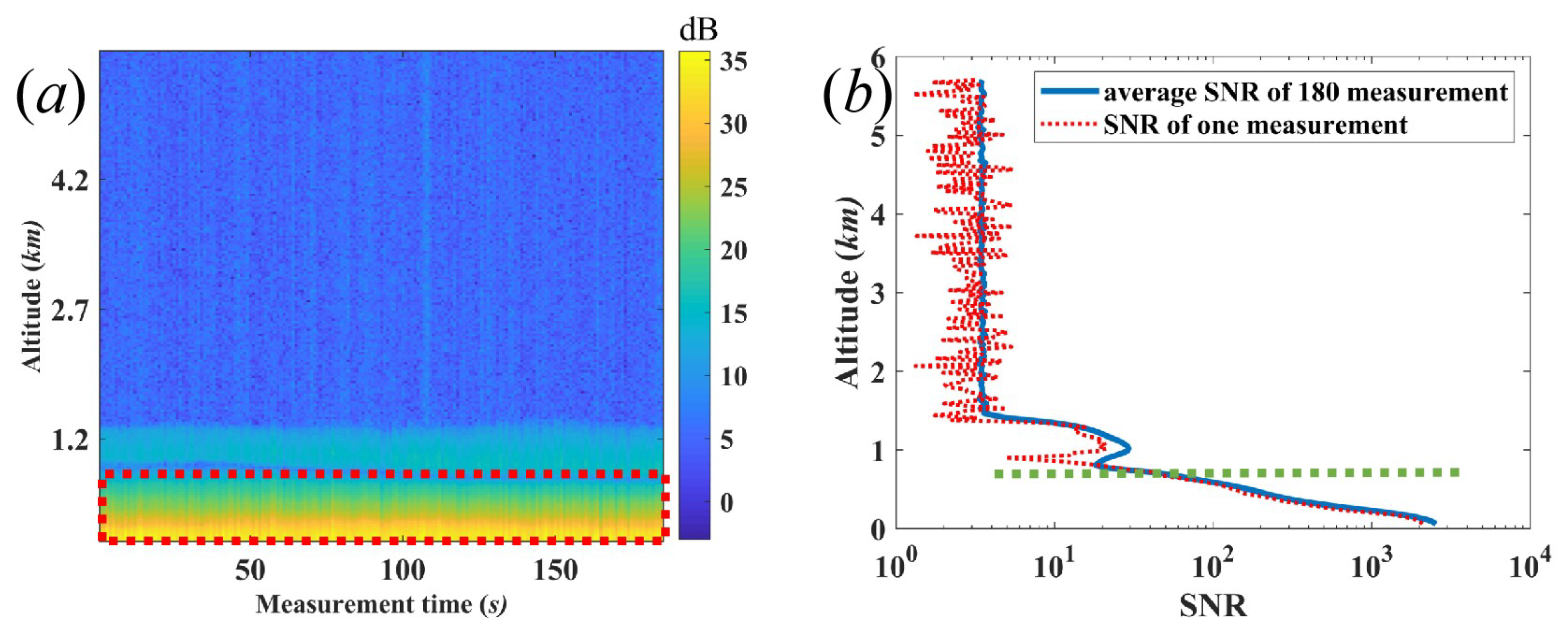
2.3. SNR of Coherent Doppler Wind Lidar (CDWL)
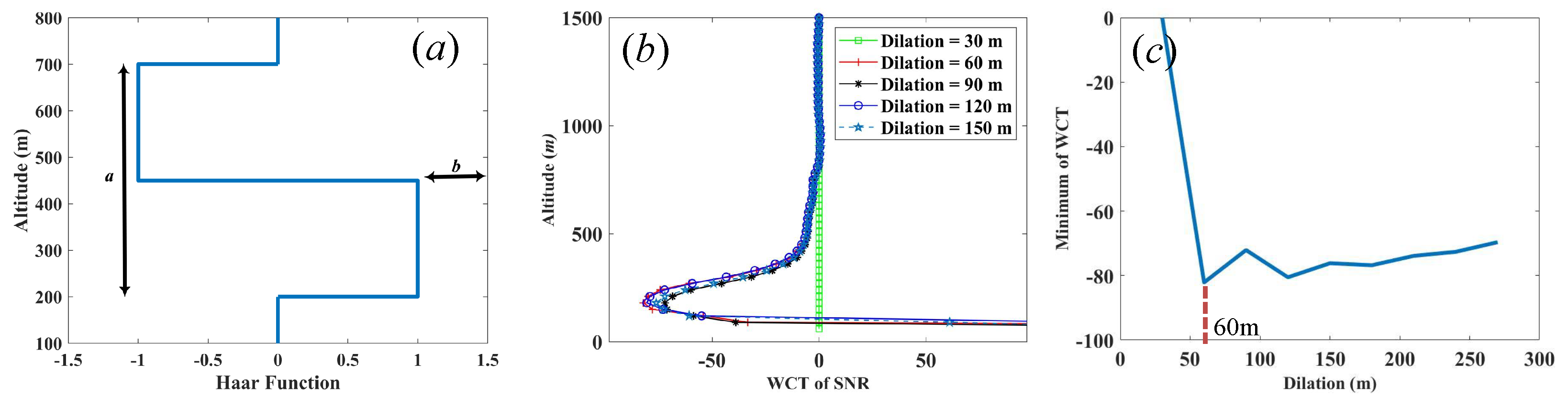
2.4. WCT
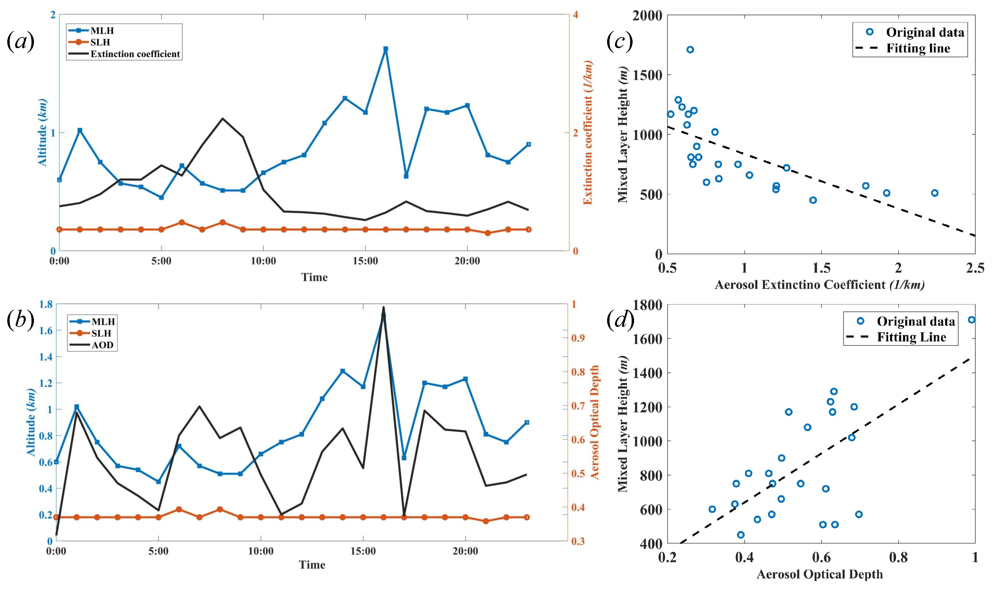
2.5. AEC and AOD
3. Results
4. Discussion
5. Conclusions
Author Contributions
Funding
Institutional Review Board Statement
Informed Consent Statement
Data Availability Statement
Conflicts of Interest
References
- Cohn, S.A.; Angevine, W.M. Boundary Layer Height and Entrainment Zone Thickness Measured by Lidars and Wind-Profiling Radars. J. Appl. Meteorol. 2000, 39, 1233–1247. [Google Scholar] [CrossRef]
- Stull, R.B. (Ed.) An Introduction to Boundary Layer Meteorology; Springer: Dordrecht, The Netherlands, 1988. [Google Scholar] [CrossRef]
- Bravo-Aranda, J.A.; de Arruda Moreira, G.; Navas-Guzmán, F.; Granados-Muñoz, M.J.; Guerrero-Rascado, J.L.; Pozo-Vázquez, D.; Arbizu-Barrena, C.; Olmo Reyes, F.J.; Mallet, M.; Alados Arboledas, L. A new methodology for PBL height estimations based on lidar depolarization measurements: Analysis and comparison against MWR and WRF model-based results. Atmos. Chem. Phys. 2017, 17, 6839–6851. [Google Scholar] [CrossRef] [Green Version]
- Dang, R.; Yang, Y.; Hu, X.M.; Wang, Z.; Zhang, S. A Review of Techniques for Diagnosing the Atmospheric Boundary Layer Height (ABLH) Using Aerosol Lidar Data. Remote Sens. 2019, 11, 1590. [Google Scholar] [CrossRef] [Green Version]
- Ma, X.; Jiang, W.; Li, H.; Ma, Y.; Jin, S.; Liu, B.; Gong, W. Variations in Nocturnal Residual Layer Height and Its Effects on Surface PM2.5 over Wuhan, China. Remote Sens. 2021, 13, 4717. [Google Scholar] [CrossRef]
- Ma, Y.; Fan, R.; Jin, S.; Ma, X.; Zhang, M.; Gong, W.; Liu, B.; Shi, Y.; Zhang, Y.; Li, H. Black Carbon over Wuhan, China: Seasonal Variations in Its Optical Properties, Radiative Forcing and Contribution to Atmospheric Aerosols. Remote Sens. 2021, 13, 3620. [Google Scholar] [CrossRef]
- Huang, A.; Ddeng, R.; Qin, Y.; Chen, Q.; Liang, Y. A Study on Remote-Sensing Inversion of Aerosol Particle Size Distributions over Yongxing Island. Acta Scient. Nat. Univ. Sunyat. 2015, 54, 138–144. [Google Scholar] [CrossRef]
- Martin, L.U. Scanning lidar measurements of surf-zone aerosol generation. Opt. Eng. 1999, 38, 250. [Google Scholar] [CrossRef]
- Zhou, S.; Wu, L.; Guo, J.; Chen, W.; Wang, X.; Zhao, J.; Cheng, Y.; Huang, Z.; Zhang, J.; Sun, Y.; et al. Measurement report: Vertical distribution of atmospheric particulate matter within the urban boundary layer in southern China—Size-segregated chemical composition and secondary formation through cloud processing and heterogeneous reactions. Atmos. Chem. Phys. 2020, 20, 6435–6453. [Google Scholar] [CrossRef]
- Salvador, P.; Pandolfi, M.; Tobías, A.; Gómez-Moreno, F.J.; Molero, F.; Barreiro, M.; Pérez, N.; Revuelta, M.A.; Marco, I.M.; Querol, X.; et al. Impact of mixing layer height variations on air pollutant concentrations and health in a European urban area: Madrid (Spain), a case study. Environ. Sci. Pollut. Res. 2020, 27, 41702–41716. [Google Scholar] [CrossRef]
- Liakakou, E.; Stavroulas, I.; Kaskaoutis, D.; Grivas, G.; Paraskevopoulou, D.; Dumka, U.; Tsagkaraki, M.; Bougiatioti, A.; Oikonomou, K.; Sciare, J.; et al. Long-term variability, source apportionment and spectral properties of black carbon at an urban background site in Athens, Greece. Atmos. Environ. 2020, 222, 117137. [Google Scholar] [CrossRef]
- Perrone, M.; Romano, S. Relationship between the planetary boundary layer height and the particle scattering coefficient at the surface. Atmos. Res. 2018, 213, 57–69. [Google Scholar] [CrossRef]
- Liu, Y.; Tang, G.; Zhou, L.; Hu, B.; Liu, B.; Li, Y.; Liu, S.; Wang, Y. Mixing layer transport flux of particulate matter in Beijing, China. Atmos. Chem. Phys. 2019, 19, 9531–9540. [Google Scholar] [CrossRef] [Green Version]
- Lou, M.; Guo, J.; Wang, L.; Xu, H.; Chen, D.; Miao, Y.; Lv, Y.; Li, Y.; Guo, X.; Ma, S.; et al. On the Relationship Between Aerosol and Boundary Layer Height in Summer in China Under Different Thermodynamic Conditions. Earth Space Sci. 2019, 6, 887–901. [Google Scholar] [CrossRef] [Green Version]
- Patil, M.; Patil, S.; Waghmare, R.; Dharmaraj, T. Planetary Boundary Layer and aerosol interactions over the Indian sub-continent. J. Atmos. Sol.-Terrestr. Phys. 2014, 112, 38–42. [Google Scholar] [CrossRef]
- Patil, M.; Patil, S.; Waghmare, R.; Dharmaraj, T. Planetary Boundary Layer height over the Indian subcontinent during extreme monsoon years. J. Atmos. Sol.-Terrestr. Phys. 2013, 92, 94–99. [Google Scholar] [CrossRef]
- Yuan, Z.; Qin, J.; Zheng, X.; Mbululo, Y. The relationship between atmospheric circulation, boundary layer and near-surface turbulence in severe fog-haze pollution periods. J. Atmos. Sol.-Terrestr. Phys. 2020, 200, 105216. [Google Scholar] [CrossRef]
- Saha, S.; Sharma, S.; Kumar, K.N.; Kumar, P.; Lal, S.; Kamat, D. Investigation of Atmospheric Boundary Layer characteristics using Ceilometer Lidar, COSMIC GPS RO satellite, Radiosonde and ERA-5 reanalysis dataset over Western Indian Region. Atmos. Res. 2022, 268, 105999. [Google Scholar] [CrossRef]
- Kotthaus, S.; Grimmond, C.S.B. Atmospheric boundary-layer characteristics from ceilometer measurements. Part 1: A new method to track mixed layer height and classify clouds. Q. J. R. Meteorol. Soc. 2018, 144, 1525–1538. [Google Scholar] [CrossRef] [Green Version]
- Uzan, L.; Egert, S.; Khain, P.; Levi, Y.; Vadislavsky, E.; Alpert, P. Ceilometers as planetary boundary layer height detectors and a corrective tool for COSMO and IFS models. Atmos. Chem. Phys. 2020, 20, 12177–12192. [Google Scholar] [CrossRef]
- Li, H.; Yang, Y.; Hu, X.M.; Huang, Z.; Wang, G.; Zhang, B.; Zhang, T. Evaluation of retrieval methods of daytime convective boundary layer height based on lidar data. J. Geophys. Res. Atmos. 2017, 122, 4578–4593. [Google Scholar] [CrossRef]
- Das, S.K.; Das, S.S.; Saha, K.; Murali Krishna, U.; Dani, K. Investigation of Kelvin-Helmholtz Instability in the boundary layer using Doppler lidar and radiosonde data. Atmos. Res. 2018, 202, 105–111. [Google Scholar] [CrossRef]
- Wang, L.; Qiang, W.; Xia, H.; Wei, T.; Yuan, J.; Jiang, P. Robust Solution for Boundary Layer Height Detections with Coherent Doppler Wind Lidar. Adv. Atmos. Sci. 2021, 38, 1920–1928. [Google Scholar] [CrossRef]
- Moreira, G.d.A.; Guerrero-Rascado, J.L.; Bravo-Aranda, J.A.; Foyo-Moreno, I.; Cazorla, A.; Alados, I.; Lyamani, H.; Landulfo, E.; Alados-Arboledas, L. Study of the planetary boundary layer height in an urban environment using a combination of microwave radiometer and ceilometer. Atmos. Res. 2020, 240, 104932. [Google Scholar] [CrossRef]
- Zhu, Z.; Zhang, M.; Huang, Y.; Zhu, B.; Han, G.; Zhang, T.; Liu, B. Characteristics of the planetary boundary layer above Wuhan, China based on CALIPSO. Atmos. Res. 2018, 214, 204–212. [Google Scholar] [CrossRef]
- de Arruda Moreira, G.; Guerrero-Rascado, J.L.; Bravo-Aranda, J.A.; Benavent-Oltra, J.A.; Ortiz-Amezcua, P.; Róman, R.; Bedoya-Velásquez, A.E.; Landulfo, E.; Alados-Arboledas, L. Study of the planetary boundary layer by microwave radiometer, elastic lidar and Doppler lidar estimations in Southern Iberian Peninsula. Atmos. Res. 2018, 213, 185–195. [Google Scholar] [CrossRef] [Green Version]
- Sawyer, V.; Li, Z. Detection, variations and intercomparison of the planetary boundary layer depth from radiosonde, lidar and infrared spectrometer. Atmos. Environ. 2013, 79, 518–528. [Google Scholar] [CrossRef]
- Bianco, L.; Wilczak, J.M. Convective Boundary Layer Depth: Improved Measurement by Doppler Radar Wind Profiler Using Fuzzy Logic Methods. J. Atmos. Ocean. Technol. 2002, 19, 1745–1758. [Google Scholar] [CrossRef]
- Zou, J.; Sun, J.; Ding, A.; Wang, M.; Guo, W.; Fu, C. Observation-based estimation of aerosol-induced reduction of planetary boundary layer height. Adv. Atmos. Sci. 2017, 34, 1057–1068. [Google Scholar] [CrossRef]
- Mao, F.; Wang, W.; Min, Q.; Gong, W. Approach for selecting boundary value to retrieve Mie-scattering lidar data based on segmentation and two-component fitting methods. Opt. Express 2015, 23, A604. [Google Scholar] [CrossRef]
- Stelmaszczyk, K.; Dell’Aglio, M.; Chudzyński, S.; Stacewicz, T.; Wöste, L. Analytical function for lidar geometrical compression form-factor calculations. Appl. Opt. 2005, 44, 1323. [Google Scholar] [CrossRef]
- Vande Hey, J.; Coupland, J.; Foo, M.H.; Richards, J.; Sandford, A. Determination of overlap in lidar systems. Appl. Opt. 2011, 50, 5791. [Google Scholar] [CrossRef] [Green Version]
- He, T.Y.; Stanič, S.; Gao, F.; Bergant, K.; Veberič, D.; Song, X.Q.; Dolžan, A. Tracking of urban aerosols using combined LIDAR-based remote sensing and ground-based measurements. Atmos. Meas. Tech. 2012, 5, 891–900. [Google Scholar] [CrossRef] [Green Version]
- Huang, X.; Ding, A.; Liu, L.; Liu, Q.; Ding, K.; Niu, X.; Nie, W.; Xu, Z.; Chi, X.; Wang, M.; et al. Effects of aerosolâĂŞ-radiation interaction on precipitation during biomass-burning season in East China. Atmos. Chem. Phys. 2016, 16, 10063–10082. [Google Scholar] [CrossRef] [Green Version]
- Wang, H.; Li, Z.; Lv, Y.; Xu, H.; Li, K.; Li, D.; Hou, W.; Zheng, F.; Wei, Y.; Ge, B. Observational study of aerosol-induced impact on planetary boundary layer based on lidar and sunphotometer in Beijing. Environ. Pollut. 2019, 252, 897–906. [Google Scholar] [CrossRef]
- Frehlich, R.G.; Kavaya, M.J. Coherent laser radar performance for general atmospheric refractive turbulence. Appl. Opt. 1991, 30, 5325. [Google Scholar] [CrossRef] [PubMed]
- Kameyama, S.; Ando, T.; Asaka, K.; Hirano, Y. Semianalytic pulsed coherent laser radar equation for coaxial and apertured systems using nearest Gaussian approximation. Appl. Opt. 2010, 49, 5169. [Google Scholar] [CrossRef] [PubMed]
- Mao, F.; Gong, W.; Song, S.; Zhu, Z. Determination of the boundary layer top from lidar backscatter profiles using a Haar wavelet method over Wuhan, China. Opt. Laser Technol. 2013, 49, 343–349. [Google Scholar] [CrossRef]
- Li, Z.F.; Li, H.; Xie, W.M.; Fan, L.L. Granulometric analysis of speckles for polarization-difference imaging in turbid media. Lasers Eng. 2011, 21, 255–263. [Google Scholar]
- Bohren, C.F.; Huffman, D.R. Absorption and Scattering of Light by Small Particles; Wiley: Weinheim, Germany, 1998. [Google Scholar] [CrossRef] [Green Version]
- People’s Republic of China. National Urban Air Quality Data of Ministry of Ecology and Environment. Available online: https://air.cnemc.cn:18007/ (accessed on 14 March 2022).
- Sedgwick, P. Pearson’s correlation coefficient. BMJ 2012, 345, e4483. [Google Scholar] [CrossRef] [Green Version]
- Chen, J.; Qian, X.; Liu, Q.; Zheng, J.; Zhu, W.; Li, X. Research on optical absorption characteristics of atmosphric aerosols at 1064 nm wavelength. Spectrosc. Spectr. Anal. 2020, 40, 2989–2995. [Google Scholar] [CrossRef]
- Inness, A.; Ades, M.; Agustí-Panareda, A.; Barré, J.; Benedictow, A.; Blechschmidt, A.M.; Dominguez, J.J.; Engelen, R.; Eskes, H.; Flemming, J.; et al. The CAMS reanalysis of atmospheric composition. Atmos. Chem. Phys. 2019, 19, 3515–3556. [Google Scholar] [CrossRef] [Green Version]


| Parameter/Unit | Value |
|---|---|
| Wavelength/nm | 1550 |
| Pulse repetition rate/kHz | 10 |
| Pulse energy/uJ | ≥150 |
| Pulse width/ns | 100 |
| Power consumption/W | <300 |
Publisher’s Note: MDPI stays neutral with regard to jurisdictional claims in published maps and institutional affiliations. |
© 2022 by the authors. Licensee MDPI, Basel, Switzerland. This article is an open access article distributed under the terms and conditions of the Creative Commons Attribution (CC BY) license (https://creativecommons.org/licenses/by/4.0/).
Share and Cite
Chen, Y.; Jin, X.; Weng, N.; Zhu, W.; Liu, Q.; Chen, J. Simultaneous Extraction of Planetary Boundary-Layer Height and Aerosol Optical Properties from Coherent Doppler Wind Lidar. Sensors 2022, 22, 3412. https://doi.org/10.3390/s22093412
Chen Y, Jin X, Weng N, Zhu W, Liu Q, Chen J. Simultaneous Extraction of Planetary Boundary-Layer Height and Aerosol Optical Properties from Coherent Doppler Wind Lidar. Sensors. 2022; 22(9):3412. https://doi.org/10.3390/s22093412
Chicago/Turabian StyleChen, Yehui, Xiaomei Jin, Ningquan Weng, Wenyue Zhu, Qing Liu, and Jie Chen. 2022. "Simultaneous Extraction of Planetary Boundary-Layer Height and Aerosol Optical Properties from Coherent Doppler Wind Lidar" Sensors 22, no. 9: 3412. https://doi.org/10.3390/s22093412