Improvement of On-Site Sensor for Simultaneous Determination of Phosphate, Silicic Acid, Nitrate plus Nitrite in Seawater

Abstract

Accurate, on-site determinations of macronutrients (phosphate (PO₄³⁻), nitrate (NO₃⁻), and silicic acid (H₄SiO₄)) in seawater in real time are essential to obtain information on their distribution, flux, and role in marine biogeochemical cycles. The development of robust sensors for long-term on-site analysis of macronutrients in seawater is a great challenge. Here, we present improvements of a commercial automated sensor for nutrients (including PO₄³⁻, H₄SiO₄, and NO₂⁻ plus NO₃⁻), suitable for a variety of aquatic environments. The sensor uses the phosphomolybdate blue method for PO₄³⁻, the silicomolybdate blue method for H₄SiO₄ and the Griess reagent method for NO₂⁻, modified with vanadium chloride as reducing agent for the determination of NO₃⁻. Here, we report the optimization of analytical conditions, including reaction time for PO₄³⁻ analysis, complexation time for H₄SiO₄ analysis, and analyte to reagent ratio for NO₃⁻ analysis. The instrument showed wide linear ranges, from 0.2 to 100 μM PO₄³⁻, between 0.2 and 100 μM H₄SiO₄, from 0.5 to 100 μM NO₃⁻, and between 0.4 and 100 μM NO₂⁻, with detection limits of 0.18 μM, 0.15 μM, 0.45 μM, and 0.35 μM for PO₄³⁻, H₄SiO₄, NO₃⁻, and NO₂⁻, respectively. The analyzer showed good precision with a relative standard deviation of 8.9% for PO₄³⁻, 4.8% for H₄SiO₄, and 7.4% for NO₂⁻ plus NO₃⁻ during routine analysis of certified reference materials (KANSO, Japan). The analyzer performed well in the field during a 46-day deployment on a pontoon in the Kiel Fjord (located in the southwestern Baltic Sea), with a water supply from a depth of 1 m. The system successfully collected 443, 440, and 409 on-site data points for PO₄³⁻, Σ(NO₃⁻ + NO₂⁻), and H₄SiO₄, respectively. Time series data agreed well with data obtained from the analysis of discretely collected samples using standard reference laboratory procedures and showed clear correlations with key hydrographic parameters throughout the deployment period.

1. Introduction

Macronutrients such as phosphate (PO₄³⁻), nitrate (NO₃⁻), and silicic acid (H₄SiO₄) play key roles in the regulation of ocean productivity and thus the marine biogeochemical carbon cycle. In particular, PO₄³⁻ and NO₃⁻ are the bioavailable forms utilized by phytoplankton and autotrophic bacteria [1,2], H₄SiO₄ exerts a strong influence on the productivity of silicifying phytoplankton such as diatoms, which are estimated to account for 40% of the total primary production in the oceans [3,4]. However, excessive input of PO₄³⁻ and NO₃⁻ into estuaries and coastal waters leads to eutrophication, deoxygenation, and other processes that damage aquatic environment [5]. In the open ocean, oligotrophic regions are subject to N and P limitation, which restricts biological productivity [6]. In tropical and subtropical regions, H₄SiO₄ is depleted to low levels of ≈0.6 μM, which limits the diatom productivity and thus carbon export from the surface mixed layer [7]. To study these biogeochemical processes, real-time and long-term monitoring of macronutrient concentrations is required to determine the spatial trends and temporal variations in their distributions [8].

Nutrient data obtained from discrete samples usually collected at operational intervals and analyzed using laboratory techniques based on automated colorimetric approaches or ion chromatography. However, such methods are labor intensive, expensive, and yield datasets with a low temporal and spatial resolution [9].

Therefore, there is an urgent need for technologies that enable on-site measurements for long-term monitoring and are equipped to cope with challenging conditions during sporadic and transient environmental events. In the last 20 years, a number of studies have been conducted on on-site monitoring of nutrients in marine waters [10,11] using mainly three analytical approaches: optical, electrochemical, and wet chemical techniques. In particular, various ultraviolet (UV) optical sensors for routine measurement of NO₃⁻ have been developed and deployed on different platforms [12,13]. These systems do not require chemical reagents, can measure over a wide range of concentrations, and are easy to use due to their small size and robustness [14]. Optical UV sensors have shown promise for long-term in situ deployment, but their application is limited by low sensitivity and accuracy due to optical interfering factors such as bromide and dissolved organic material [15].

Electrochemical techniques for nutrient measurements facilitate sensor miniaturization, require low power, and in some cases eliminate the need for reagents. Two electrochemical sensors have been reported for H₄SiO₄ [16,17,18] and PO₄³⁻ [19,20]. In these sensors, molybdate (MoO₄²⁻) ions are introduced into a working solution (NaCl solution (34.5 g L⁻¹)) by electrochemical oxidation of a solid Mo wire. Then, either a silicomolybdate or a phosphomolybdate complex is electrochemically produced on an Au working electrode using cyclic voltammetry or square wave voltammetry. Although a short period of a few minutes is required for the electrochemical measurements, a longer period of 30 min is required for PO₄³⁻ measurements [14]. These techniques seem promising for long-term deployment due to absence of liquid reagents, but further development and investigation is needed for field applications.

Wet chemical methods, also known as reagent-based colorimetric methods, have been used in several on-site sensors deployed in rivers, estuaries, coastal waters, and oceans. These methods involve the formation of a light-absorbing dye that provides a robust measurement tool for nutrients with low detection limits and good precision. Among the more recent technologies used for in situ monitoring based on colorimetric assays is the implementation of microfluidics in lab-on-a-chip devices (LOC) [21,22]. Although the LOC technology has shown better performance in terms of lower reagent consumption, lower power consumption, and smaller size compared to other commercially available in-situ analyzers, a multiparameter instrument LOC is not available, and the cost of sensors is relatively high.

Several colorimetric sensors based on flow injection analysis (FIA) have been reported. A submersible chemical analyzer known as Analyseur Chimique In Situ (ALCHIMIST) was installed on a remotely operated vehicle for in situ determination of Σ(NO₃⁻ + NO₂⁻) and total dissolved sulfide [23]. NAS2E was used for monitoring of Σ(NO₃⁻ + NO₂⁻), and the NH4-Digiscan in situ analyzer was used for monitoring ammonium (NH₄⁺) in coastal and estuarine waters. Other commercially available colorimetric in situ sensors and systems include the Autonomous Profiling Nutrient Analyzer (APNA) and ChemFIN (SubChem Systems, Inc., Narragansett, RI, USA) for NO₃⁻ and Σ(NO₃⁻ + NO₂⁻) analysis, and HydroCycle (Sea-Bird Scientific, Philomath, OR, U S) for PO₄³⁻. Other systems are based on either the micro loop flow analysis (µLFA) (WIZ, SYSTEA S.p.A., Anagni, Latium, Italy) [24,25] or reverse flow analysis such as the autonomous nutrient analysis in situ (ANAIS) [26].

Recently, new paper-based microfluidic devices for the determination of macronutrients in natural waters have been reported [27,28]. The techniques are based on fluid flow through paper by capillary action without the need for a pump. In principle, the device consists of a sample port into which the water sample is introduced and transport channels connecting other parts of the device, such as the reaction zone, where the analyte solution mixes or reacts with the reagents. The signal (i.e., color formation) is subsequently formed in the detection zone and can be quantified using a cell phone or desktop scanner. Although the proposed systems offer promising applications for on-site observations of nutrients in natural waters, the technique does not allow for autonomous continuous monitoring.

All reported wet chemical in situ analyzers are designed to observe single nutrient, and therefore cannot perform multinutrient analysis with the same instrument. An exception is the WIZ probe, but there are no reports in the literature of long-term field testing of these multi-nutrient sensors.

FIA systems based on a single syringe pump and a multiposition switching valve are excellent at compensating for the shortcomings of the continuous flow analyzers currently in use [29,30,31], as they are capable of delivering a small volume (at a level of 10 µL) of reagent without using peristaltic pumps [32]. Automated syringe pump FIA instruments have been developed by EnviroTech LLC (Chesapeake, VA, USA) for on-site DNA in situ determination of Σ(NO₃⁻ + NO₂⁻), PO₄³⁻, as well as H₄SiO₄ based on the Griess reaction [33] using a Cd column as the reducing agent for NO₃⁻, the classical blue phosphomolybdate method [34], and the classical silicomolybdate method [35]. The instruments perform routine chemical analyzes according to a preloaded protocol stored in their firmware. However, the protocols show a poor performance and precision, which limits their use for environmental applications in the field. In the stored protocol, only one standard was used for each nutrient. There is no matrix effect correction (i.e., no optical correction) in the sample concentration calculation, as described in the Data Processing Protocol section of the User’s Guide, which limits the use of the analyzer in field deployments. The conventional cadmium column reduction procedure for nitrate determination, which requires regular regeneration, and the rate at which reagents and standards are consumed per measurement, also limit its use for long-term field use.

To the best of our knowledge, there are very few studies that have demonstrated multi-macronutrient analyzers for long periods of deployment. In the present work, we improve the performance of such an instrument by implementing a new nitrate method that uses vanadium chloride (VCl₃) for the reduction of NO₃⁻ to NO₂⁻. This method has been used for a decade in flow analyzers for on-site monitoring of nitrate in natural waters [36,37,38]. It showed more promising performance for long-term use than the classic copper-coated cadmium column or zinc particles reported by Ellis et al. in 2011, which must be replaced daily due to reduction efficiency degradation [39]. It also reduces the reagent consumption, which increases the endurance of the sensor for longer deployment. The optimized method was tested during a deployment in coastal waters of the Kiel Fjord, Germany. The new method is validated by additional discrete sampling during the deployment and analysis using a reference air segmented flow analyzer.

2. Materials and Methods

2.1. Reagents and Standards Preparation

The reagents used in this study were analytical-grade salts prepared with deionized water (resistivity >18.2 MΩ-cm, Milli-Q, MilliporeSigma, Burlington, MA, USA). All glass and plasticware were routinely cleaned, rinsed with deionized water, soaked in 1 M HCl (37%, Carl Roth, Karlsruhe, Germany) for more than 24 h, rinsed with deionized water, and stored in plastic bags before use.

The reagents for PO₄³⁻ determination were prepared as follows.

-

The acidic MoO₄²⁻ reagent (R1) was prepared by dissolving 12.8 g ammonium molybdate tetrahydrate ((NH₄)₆Mo₇O₂₄ 4H₂O, Sigma Aldrich, Burlington, MA, USA) and 140 mL sulfuric acid (H₂SO₄, 98%, Merck, Kenilworth, NJ, USA) to obtain a concentration of 2.57 M (pH 0.6), 3.5 mL of a solution of potassium antimony (III) oxide tartrate trihydrate (PAT; C₈H₄K₂O₁₂Sb₂ 3H₂O; Merck) (5.3 g/100 mL deionized water), and 1 mL of solution of sodium dodecyl sulfate (C₁₂H₂₅OSO₂ONa; Merck, Kenilworth, NJ, USA) (30 g/L) in 1000 mL deionized water.

-

Ascorbic acid reagent (R2) was prepared by dissolving 25 g of L(+)-ascorbic acid (C₆H₈O₆; ≥99%, Carl Roth, Karlsruhe, Germany) in 1000 mL of deionized water.

The reagents for H₄SiO₄ determination were prepared as follows:

-

The MoO₄²⁻ reagent (R1) was prepared by dissolving 15 g of ammonium molybdate tetrahydrate, 5.4 mL of H₂SO₄, and 1 mL of sodium dodecyl sulfate solution in 1000 mL of deionized water.

-

The oxalic acid reagent (R2) was prepared by dissolving 50 g of oxalic acid dihydrate (C₂H₂O₄.2H₂O; ≥99%, Carl Roth, Karlsruhe, Germany) into 1000 mL of deionized water.

-

The ascorbic acid reagent (R3) was the same as that used for PO₄³⁻ determination.

The reagents for NO₃⁻ and NO₂⁻ determination were prepared as follows:

-

The Griess reagent and VCl₃ reducing agent reagent were prepared by dissolving 5 g of VCl₃ (Sigma Aldrich, Burlington, MA, USA) in 200 mL of deionized water until the solution turned a dark brown color. Then, 15 mL of concentrated HCl (37%, trace-metal grade, Fisher Scientific, Waltham, MA, USA) was added. After a dark-turquoise color appeared, 10 g of sulfanilamide (H₂NC₆H₄SO₂NH₂; Merck, USA) was added by dissolving 1 g of N-(1-naphthyl) ethylenediamine dihydrochloride (C₁₀H₇NHCH₂CH₂NH₂.2HCl; Merck, Kenilworth, NJ, USA) and 1 mL of a solution of Triton x-100 50% (v/v) (50 mL Triton x-100 (Sigma Aldrich, Burlington, MA, USA): 50 mL isopropanol (Fisher Scientific, Waltham, MA, USA) in 1000 mL of deionized water.

Stock solutions of PO₄³⁻ (1 mM) were prepared by dissolving 0.136 g of potassium dihydrogen sulfate (KH₂PO₄; Merck, Kenilworth, NJ, USA) into 1000 mL of deionized water. Stock solutions of H₄SiO₄ (1 mM) were prepared by dissolving 0.0212 g of sodium metasilicate pentahydrate (Na₂SiO₃.5H₂O; Sigma Aldrich, city, state, USA) into 1000 mL of deionized water. Stock solutions of NO₃⁻ (1 mM) were prepared by dissolving 0.0849 g of sodium nitrate (NaNO₃; Merck, Kenilworth, NJ, USA) into 1000 mL of deionized water. Stock solutions of NO₂⁻ (1 mM) were prepared by dissolving 0.0689 g of sodium nitrite (NaNO₂; Merck, Kenilworth, NJ, USA) into 1000 mL of deionized water.

Standard PO₄³⁻, H₄SiO₄, NO₃⁻, and NO₃⁻ calibration solutions were prepared by further diluting the respective stock solutions with deionized water.

All reagent solutions were stored in brown 500 mL high-density polyethylene (HDPE) laboratory-grade bottles (Nalgene, Thermo Scientific, Waltham, MA, USA) and kept refrigerated when not in use. Blank, standard, and cleaning solutions were freshly prepared prior to field use and stored in 1000 mL HDPE Nalgene bottles.

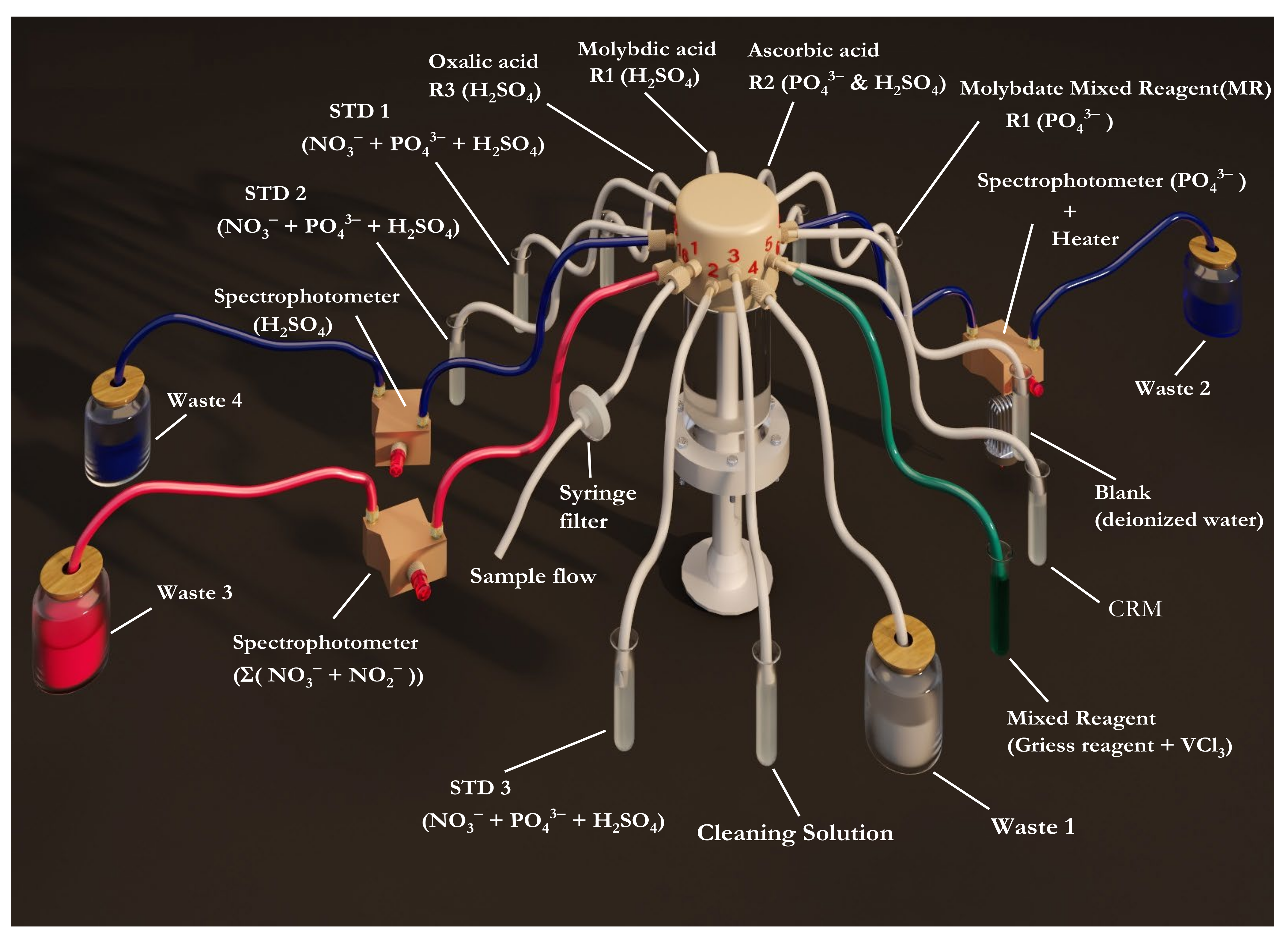
2.2. Multinutrient Analyzer Description

The analyzer (AutoLAB, EnviroTech LLC, Chesapeake, VA, USA) was a multichannel on-site portable chemical analyzer that automatically measures the concentrations of nutrients (Σ(NO₃⁻ + NO₂⁻), PO₄³⁻, and H₄SiO₄) in natural waters using wet chemical techniques with colorimetric detection. The system consisted of four main parts, namely, a 16-way rotary valve, a stepper motor-driven syringe, 3 colorimetric detectors, and an electronic controller in a single housing (Figure 1). The rotary valve and the syringe (≈2.2 mL full motion) were driven by a stepper motor controlled by an internal program stored on a memory card and displayed on a terminal interface (Tera Term). A blank, sample, or standard is collected by the analyzer by retracting the syringe plunger while the rotary valve is at the inlet position. Switching the rotary valve and retracting the plunger allows the reagent to be added to the analyte, causing a chemical reaction. This changes the color of the solution contained in the syringe according to the concentration of the nutrient.

The colorimetric detector consisted of a narrow capillary flow cell made of high-grade glass (1 cm path length for the Σ(NO₃⁻ + NO₂⁻) and PO₄³⁻ detector and 2 cm path length for the H₄SiO₄ detector with a light-emitting diode (LED) as the light source on one side and a photodiode detector on the opposite side. An additional monitoring photodiode was positioned next to the LED to monitor the intensity of the light source. Green LED with a peak wavelength of 567 nm and a silicon photodiode with a peak intensity at a wavelength of 570 nm were used for Σ(NO₃⁻ + NO₂⁻). No information on LED or photodiodes of PO₄³⁻ or H₄SiO₄ detectors was given in the operating manual. To minimize light interference from the outside, the colorimeters were encapsulated in polyurethane. Inside the electronics housing was a series of electronic modules: the main control unit and the motor drivers and detector interfaces. Both the motor drivers and detector interfaces had their own microprocessors and were controlled by the main control unit via a link. Four devices (syringe motor, valve motor, phosphate detector, and (nitrate + nitrite) and silicic acid detectors) were configured through an arrangement called a serial peripheral system (SPS), where the detectors and motors are referred to as SPS devices, and each device had its own SPS address, which is called in the internal scripting language.

The syringe had a polyetheretherketone (PEEK) plunger in a glass cylinder that was fitted with an O-ring. The valve was made of PEEK with a linear polytetrafluoroethylene (PTFE). The swivel fittings were provided with barbed adapters to connect the pump tubing (Tygon LMT-55; green-green, inner diameter 1.85 mm) for fluid transfer. The 0.5 mm PTFE tubing and 1/4 28″ fittings were used to connect the valve to the detector. The same tubing and fittings were used for the sample, connecting via a 1/4 28″ Luer adapter (female–male) PEEK.

2.3. Chemical Methods

2.3.1. Phosphate Chemical Assay

The conventional blue method was employed here to quantify PO₄³⁻ involving a direct reaction with orthophosphate in an acidic MoO₄²⁻ solution in the presence of PAT to form the yellow phosphomolybdate complex H₃PO₄ (MoO₃)₁₂. This solution was then reduced by ascorbic acid as a reducing agent to form the deep blue-colored phosphomolybdate complex [H₄PMo₈^(VI)Mo₄^(V)O₄₀]³⁻, with extinction measured at a wavelength of 880 nm.

H₄SiO₄ has the same tendency to react with MoO₄²⁻ to form a silicomolybdate complex that adsorbs at 880 nm, interfering with PO₄³⁻ analysis in seawater. A pH of 0.4–0.9 with a proton/molybdate (H⁺/MoO₄²⁻) ratio of 60–80 minimizes the interference of H₄SiO₄ in the analysis of PO₄³⁻ [40,41].

2.3.2. Silicic Acid Chemical Assay

The determination of the H₄SiO₄ is similar to that of PO₄³⁻. In particular, it is based on the reaction of H₄SiO₄ with MoO₄²⁻ under acidic conditions of pH 1.5–2 to form the yellow complex H₃SiO₄ (MoO₃)₁₂ after a complexation time of 180 s. The solution is then reduced by ascorbic acid in the presence of oxalic acid, which acts as a masking agent for PO₄³⁻ to form a deep blue colored product with maximum absorbance at a wavelength of 880 nm.

2.3.3. Nitrate and Nitrite Chemical Assay

The determination of NO₃⁻ and NO₂⁻ is based on the reduction of NO₃⁻ to NO₂⁻ using VCl₃ at elevated temperatures (≈50 °C) for 30 min. The reduced NO₃⁻ plus NO₂⁻ originally present in the sample was quantified by using the Griess reagent method. This method is based on the diazotization of NO₂⁻ with sulfanilamide to form a diazonium salt, which is then reacted with the coupling agent N-(1-naphthyl) ethylenediamine dihydrochloride (NED) to form a pink azo dye with maximum absorbance at a wavelength of 540 nm. The mixed reagent (Griess reagent + VCl₃) allows for the determination of both NO₂⁻ and Σ(NO₃⁻ + NO₂⁻) and thus the calculation of NO₃⁻ with the same detector. The reaction mixture can be sent to the detector for NO₂⁻ determination before the heating step, while Σ(NO₃⁻ + NO₂⁻) is determined after the reduction and heating steps.

2.4. Analytical Protocol

The complete measurement cycle for each nutrient [PO₄³⁻, H₄SiO₄, or Σ(NO₃⁻ + NO₂⁻)] begins with a calibration that includes a blank and three mixed standards with known concentrations of PO₄³⁻, H₄SiO₄, and NO₃⁻ followed by the analysis of the samples. For each nutrient cycle, after analysis of the highest concentrated standard and samples, a solution of 0.1 M NaOH + 0.5 mL L⁻¹ 50 Triton X-100 was drawn into the syringe to wash the system and minimize carryover effects. During the washing step, the three detectors were used to assess the cleaning of the analyzer. To prevent carryover between the solutions during sample analysis, the syringe and colorimeter were flushed twice with 2 mL of either the blank or the standard and six times with 2 mL of the seawater sample. For the PO₄³⁻ measurement, the analytical protocol involved the drawing of the analyte solution and the two reagents into the syringe in a volumetric ratio of 4:1:1. Mixing was performed by four consecutive back and forth movements of the syringe plunger, which allowed for the initial color to develop. Then, the syringe injected the solution into the detector, allowing the color development to fully develop for 180 s. Finally, the light intensity of the color formed was measured. For the H₄SiO₄ measurement, the analyte solution was mixed with the three reagents in a ratio of 1:1:1:1. The analyte solution was mixed with the MoO₄²⁻ reagent in the syringe, and the flow was stopped for 180 s to allow the yellow complex to form before mixing with the other two reagents. Finally, the solution was transferred to the colorimeter for color determination. For NO₃⁻ and NO₂⁻ measurement, the analyte solution was mixed with the modified Griess reagent at a volumetric ratio of 2:1. The solution was then passed into the PO₄³⁻ detector, where it was incubated at an elevated temperature (≈50 °C) for 30 min. The solution was then transferred to the Σ(NO₃⁻ + NO₂⁻) detector for colorimetric determination. For a single sample measurement, a total volume of 137 μL of reagents (i.e., mixed molybdate reagent and ascorbic acid) was used for PO₄³⁻ determination, a total volume of 396 μL of reagents (i.e., molybdate reagent, oxalic acid reagent, and ascorbic acid reagent) for H₄SiO₄ determination, and a total volume of 137 μL of Griess reagent containing vanadium chloride for Σ(NO₃⁻ + NO₂⁻) determination was required. A schematic diagram of the syringe pump and the rotary valves is shown in Figure 2. The detailed steps for the nutrient measurement protocol are described in Table S1 and Video S1 [42].

2.5. Data Processing

The absorbance of the blank, standard, and sample was calculated by using the following equation:

$$\mathrm{Absorbance}=-lo{g}_{10 }\left(\frac{V}{V^R}\times \frac{V_0^R}{V_0}\right),$$

(1)

where $V$ is the voltage of the measuring photodiode (intensity of transmitted light) and $V_0$ is the voltage of the monitoring photodiode (intensity of incident light) for the analyte solution after color formation, and $V^R$ and $V_0^R$ are the voltages of the measuring photodiode and the monitoring photodiode for the analyte solution before the reagent was added, respectively. A linear regression between the absorbance of the blank and the three standards was assessed after every 10 measurements. The sample concentration (µM PO₄³⁻, µM SiO₄⁴⁻, or µM Σ(NO₃⁻ + NO₂⁻)) was calculated by the following equation:

$$\mathrm{Concentration} \left(\mu \mathrm{M}\right)=\left(A-B\right)/S,$$

(2)

where $A$ is the absorbance of the sample, $B$ is the intercept of the linear fit in the absorbance unit (AU), and $S$ is the slope of calibration curve (AU) µM⁻¹.

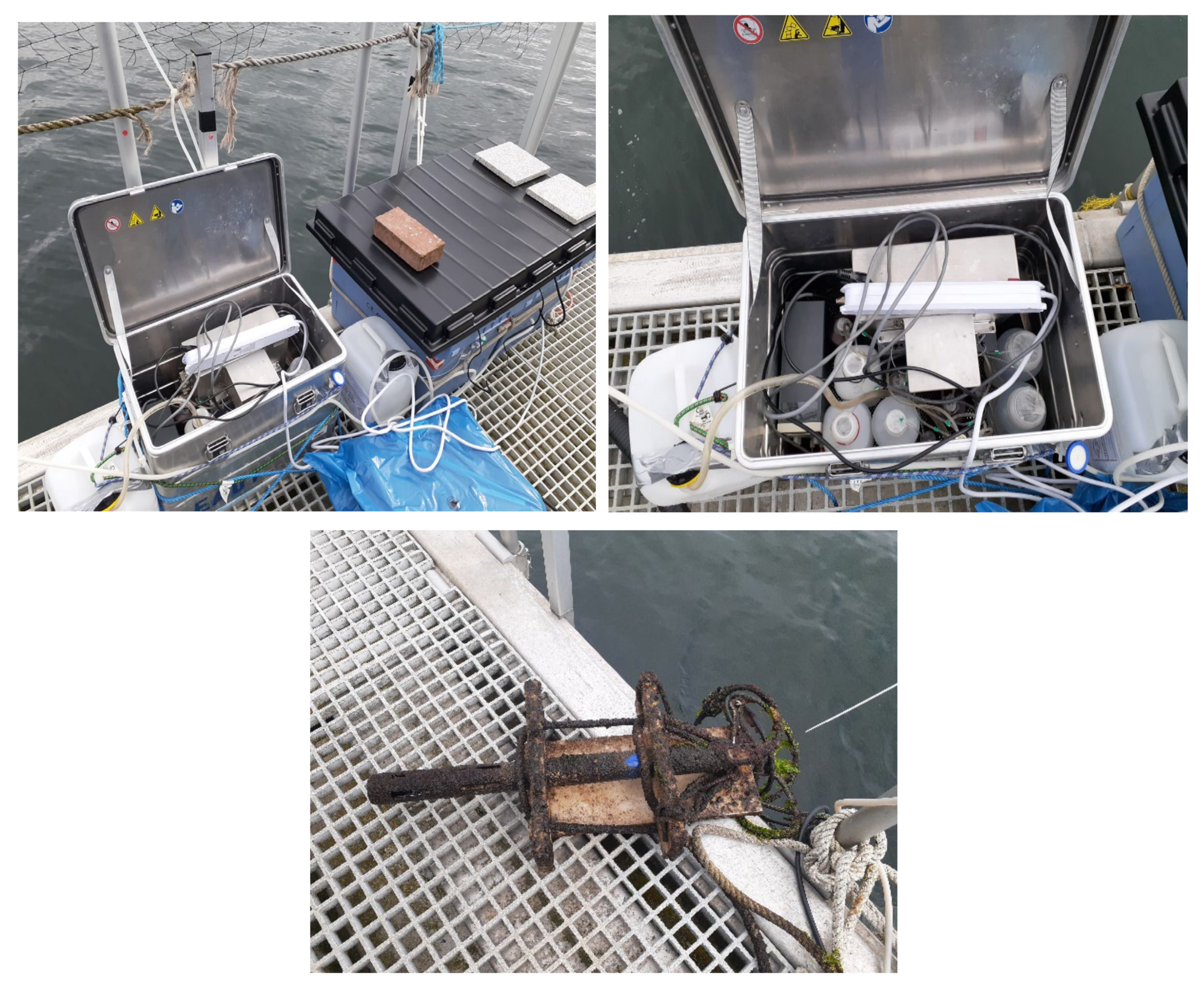
2.6. Field Deployment and Discrete Sampling

A field deployment was conducted on a pontoon in Kiel Fjord, southwestern Baltic Sea, Germany, in May–June 2021. The analyzer was housed in a weather-proof aluminum container (Zarges, Weilheim, Germany) that was placed on the pontoon (Figure 3). The analyzer was fed with a continuous water flow from a depth of 1 m using a submerged water pump with an output of 600 L/h and power consumption of 8 W (Eheim, Deizisau, Germany). The pump inlet was protected by a Cu net (mesh size ≈ 0.297 mm). The water flow was diverted to the analyzer’s sample inlet through a 0.45 μm polyethersulfone syringe filter (Millipore). The analyzer was equipped with a blank solution and three standard solutions for NO₃⁻ (1, 5, and 10 μM), PO₄³⁻ (0.5, 1, and 2 μM), and H₄SiO₄ (1, 10, and 20 μM), all prepared in artificial seawater (17 g L⁻¹ NaCl). After every 10 sample measurements, a calibration procedure was performed. A multiparameter sonde EXO2 (YSI, Yellow Springs, OH, USA) was deployed beside the analyzer to monitor salinity, temperature, and dissolved oxygen (DO). The EXO2 Sonde was deployed on 22 May at a depth of 1 m and sampling frequency of 1 min. Discrete samples were collected from the outlet of the pump filtered through a 0.45 µm syringe filter connected to a 60 mL acid-washed plastic syringe into acid pre-washed 15 mL low-density polypropylene tubes (SEAL Analytical Ltd., Southampton, UK) The collected samples were immediately frozen for later analysis using a QuAAtro continuous air segmented flow analyzer (SEAL Analytical Ltd.). Ancillary data such as wind speed, water temperature, rain precipitation, and solar radiation were obtained from the GEOMAR weather station positioned near the deployment site [43].

3. Results and Discussion

3.1. Optimization of Analytical Conditions

Different analytical conditions were studied to obtain the highest possible sensitivity for the nutrient measurements. The influence of key analytical parameters was evaluated, including reaction time for PO₄³⁻, complexation time for H₄SiO₄, and analyte/reagent ratio for NO₃⁻. For PO₄³⁻, the reaction time was identified as the period between the stopping of the flow and the color development of the reaction mixture in the measurement flow cell. The reaction time varied from 0 to 300 s, and the analytical sensitivity was calculated from the absorbance values of the blank solution and two standard solutions (1 and 2 µM PO₄³⁻) (Figure 4a). With an increase in reaction times, the analytical sensitivity increased from 0.0058 (±0.0025) AU µM⁻¹ and an RSD of 43.9% for 0 s to 0.173 (±0.0002) AU µM⁻¹ and 1.19% RSD for 120 s. Sensitivity continued to increase at 180 s with a mean value of 0.0181 (±0.0004) AU µM⁻¹ and RSD of 2.41%. A slight decrease was observed at 240 s with a value of 0.0173 (±0.0011) AU µM⁻¹ and an RSD of 6.22%. The maximum sensitivity was reached at 300 s with a mean value of 0.021 (±0.0045) AU µM⁻¹ and an RSD of 21.9%. On the basis of the highest sensitivity value and the lower RSD value (5% level), 180 s was chosen as the optimal reaction time.

For H₄SiO₄, the complexation time was identified as the time during which the analyte and Mo reagent reacted in the syringe and thus the time before the addition of the other two reagents (oxalic acid and ascorbic acid). Increased analytical sensitivity was observed with an increase in the complexation time from 0 s (0.0095 ± 0.00042) AU µM⁻¹ and an RSD of 4.39% to 300 s (0.0181 ± 0.000436) AU µM⁻¹ and an RSD of 2.4%. With an RSD value of 1.54%, and a change in analytical sensitivity (Δs) of 0.0068 AU µM⁻¹ from 0 s to 120 s and Δs of 0.0018 AU µM⁻¹ from 120 s to 300 s, 120 s was chosen as the optimal time for complexation. This shows good sensitivity with a low RSD for 120 s and no further improvement for complexation times of up to 300 s (Figure 4b).

For NO₃⁻ measurements, the reaction temperature is crucial [44,45]. We set the temperature to the maximum value (≈50 °C) and tested the reduction time from 20 min to 50 min (Figure S1). An improvement in reduction efficiency was obtained when we increased the reduction time from 20 min (61%) to 30 min (63%), while no further improvement was noted when the reaction time was increased to 50 min. Therefore, 30 min was chosen as the optimal reaction time. The analyte/reagent ratio was also investigated, and the maximum sensitivity was obtained at a ratio of 2:1 with a value of 0.054 AU µM⁻¹. The results were plotted against the ratio of absorbances values of NO₃⁻ and NO₂⁻ of the same concentration (to obtain reduction efficiency). As shown in Figure 4c, the efficiency gradually decreased from a ratio of 1:1 (69%) to reach 66.8% at a ratio of 1:6, and then increased at a ratio of 2:1 (76.5%) and before decreasing again at a ratio of 4:1 (73.5%). On the basis of these results, a 2:1 ratio of analyte/reagent was chosen as optimal.

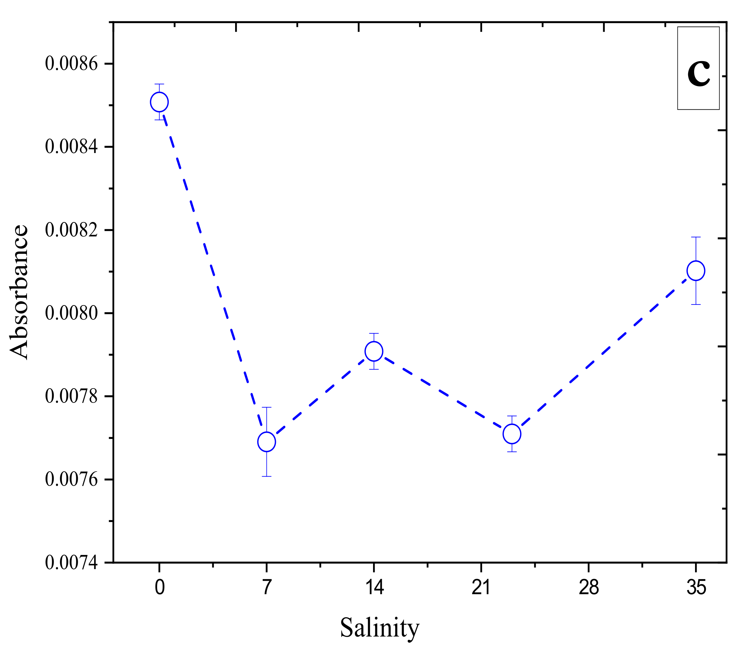
3.2. Effect of Salinity

Large variations in salinity were observed in estuaries and coastal waters compared to freshwater and open oceans, and these can affect the measurement of nutrients due to matrix differences. The effect of salinity on the analytical sensitivity of colorimetric measurements can be illustrated by two aspects. The first is the difference in refractive index between the saline sample and fresh water due to the salt effect, referred to as the Schlieren effect. The second is the effect of ionic strength on the analytical sensitivity. These effects occur at high salinity when the transmitted light is directed to the monitoring photodiode [46].

When the flow cell is filled with seawater, a lower voltage is measured by the photodiode than with deionized water. As a result, for the same analyte concentration, lower absorbance values were obtained for the samples in a seawater matrix compared to those in the deionized water matrix. Equation (1) was used to calculate the absorbance offset, which was corrected by subtracting this offset from the sample absorbance after color development.

Salinity variations have an effect on the chemistry used for each nutrient species. The Griess reaction, which involves reduction of nitrate based on VCl₃, is strongly affected by salinity fluctuations [36]. To investigate the influence of the salinity variations on the analytical sensitivity, the determination of a standard solution of 5 µM NO₃⁻ was used for solutions with different salinity values that were prepared by dissolving different amounts of NaCl in deionized water. Figure 5a shows an absorbance of 5 µM NO₃⁻ in deionized water S = 0 (0.14 AU), with absorbance values decreasing with increasing salinity from S = 7 (0.105 AU) to S = 14 (0.09 AU). A steady state was reached with increasing salinity to S = 23 (0.09 AU) and to S = 35 (0.09 AU).

The influence of salinity variations on the analytical sensitivity in H₄SiO₄ measurements has been reported [47], with a reported molar absorptivity of the silicomolybdate blue complex in distilled water of 22 × 10³ L mole⁻¹ cm⁻¹ and in oceanic seawater of 19 × 10³ L mole⁻¹ cm⁻¹. Figure 5b shows the absorbance of 5 µM H₄SiO₄ in deionized water S = 0 (0.07 AU) with a higher value compared to salinities ranging from S = 23 (0.06 AU) to S = 35 (0.005 AU).

The analytical sensitivity of the Mo-Blue method for PO₄³⁻ is not affected by the variation in the salinity of the sample matrix [48,49]. The Schlieren effect is the bias that generally occurs in the analytical signal when onboard blank and standard solutions with different salinities than the seawater samples used [50]. This is evident when comparing the analytical sensitivity of 1 µM PO₄³⁻ standard in a solution of deionized water (S = 0) (0.008 AU) with that using a solution of S = 7 (0.008 AU). Although no large bias was observed when comparing samples with different salinities of S = 7–35 (Figure 5c), an RSD value of 2.11% was noted. Variations in salinity had little effect on analytical sensitivity after applying the optical correction based on Equation (1) compared to values obtained without optical correlation (i.e., via the traditional Beer’s law equation $A=-lo{g}_{10 }\left(\frac{V}{V_0}\right)$), where $V$ is the voltage of the measuring photodiode (intensity of transmitted light) and $V_0$ is the voltage of the monitoring photodiode (intensity of incident light).

We attempted to correct for the salinity error during measurement by taking the photodiode measurement for the analyte solution before addition of the reagents. Figure S2 shows the measured concentrations of 5 µM NO₃⁻ (Figure S2a), 5 µM H₄SiO₄ (Figure S2b), and 1 µM PO₄³⁻ (Figure S2c). The values obtained with the traditional Beer’s law equation are shown as red circles, while those obtained with Equation (1) using the optical correction are shown as black circles. The comparison between the two values showed that the values obtained with the traditional Beer’s law were underestimated by 3.95% (S = 0) for 5 µM NO₃⁻ compared to values obtained with the optical correction, with the underestimation increasing with increasing salinity to 40.6% (S = 23 and S = 35). An underestimation of 2.5% (S = 0) was found for 5 µM H₄SiO₄, increasing to 43.9% (S = 35) with increasing salinity. An underestimation of 1.42% (S = 0) was found for 1 µM PO₄³⁻, increasing to 16.4% (S = 35) with increasing salinity. Despite the optical correction, it is recommended to use standards with salinity close to that of the studied waters for field work on board.

3.3. Analytical Performance

The analytical performance of the analyzer was tested by evaluating a series of calibrations (Figure 6). The calibration plot showed measurements in deionized water spiked with 0.2, 0.5, 0.75, 1, 2, 5, 10, 20, 40, 60, and 100 µM PO₄³⁻. The calibration plot showed an analytical sensitivity of 0.01211 AU µM⁻¹, indicating good linearity over a wide range (0.2–100 µM) of PO₄³⁻ with a coefficient of determination R² of 0.999. For H₄SiO₄, deionized water was spiked with a range of H₄SiO₄ standards (0.2, 0.5, 0.75, 1, 2, 5, 10, 20, 40, 60, and 100 µM SiO₄⁻⁴). The calibration plot showed a sensitivity of 0.02377 AU µM⁻¹ with a good linearity over a wide range (up to 100 μM) of H₄SiO₄ with R² = 0.992. For NO₃⁻ and NO₂⁻, the calibration plots showed analytical sensitivities of 0.00614 and 0.01202 AU µM⁻¹ for NO₃⁻ and NO₂⁻, respectively, and broad linear ranges of 0.5–100 µM for NO₃⁻ and 0.4–100 µM for NO₂⁻ with R² = 0.998 and 0.995, respectively. The values of the intercepts and slopes of the corresponding calibration curves are presented in Table S2; standard deviation values, static t-values, and probabilities are also reported, and the data showed that all values were significant (p < 0.01), except for the intercept of the calibration curve for silicic acid, because the blank measurements for silicic acid in deionized water showed negative values [51].

The limit of detection (LOD) was calculated as 0.18 μM, 0.15 μM, 0.45 μM, and 0.269 μM, and the limit of quantification (LOQ) was calculated as follows: 0.6 µM 0.3 µM, 1.5 µM, and 0.89 µM for PO₄³⁻, H₄SiO₄, NO₃⁻, and NO₂⁻, respectively, where LOD and LOQ were calculated according to IUPAC recommendation [52,53] using the following equations:

$$\mathrm{LOD}=3 \sigma ,$$

(3)

$$\mathrm{LOQ}=10 \sigma ,$$

(4)

where $\sigma$ is defined as the standard deviation of blank measurements (n = 10) (blank measurements were made by applying the associated calibration curves of the blank signals).

Technically, the analyzer can detect nitrite in the field, as we described in the Materials and Methods. However, nitrite concentrations in natural waters are typically in the nanomolar range and below our reported LOD, which limits the use of our analyzer to detect nitrite and nitrate separately.

Table 1 indicates the figures of merit of the analyzer following our analytical improvements and compares the performance with other portable on-site analyzers reported in the literature and/or commercially available (WIZ [25], APNA [52], Hydrocycle PO4 [53], NAS3X [54], ANAIS [26], ALCHEMIST [23], NuLAB [55], and Lab on Chip (LOC) [56,57,58], as well as other UV spectral sensors for NO₃⁻ such as SUNA [59], OPUS [13,60], and SUV-6 [61]). The WIZ, APNA, NAS3X, ANAIS, and NuLAB devices are the only multi-nutrient analyzers reported to date. Although they have a number of advantages, there are some limitations to their application in the field. The sensitivity of WIZ analyzers is limited by their high variability at low concentrations. APNA and ANAIS provide four separate units for PO₄³⁻, H₄SiO₄, and NO₃⁻ or Σ(NO₃⁻ + NO₂⁻). APNA and ChemFIN are based on continuous flow injection analysis, in which the sample and reagent are introduced into a carrier stream, resulting in greater dispersion of the sample and affecting long-term sensitivity [62]. ANAIS is based on reverse injection analysis, in which the detection reagent is injected into the mobile phase of the sample, which reduces sample dispersion and ensures high sensitivity over a long period of time. However, this type of FIA still suffers from the fact that detection is performed under non-equilibrium conditions, which reduces sensitivity compared to manual methods [63]. NAS3X and NuLAB are based on the same type of FIA as the AutoLAB method, where a syringe pump and multi-position ports for reagent and sample delivery combine the features of continuous flow analysis with low reagent and sample consumption with the advantages of discrete (batch) sampling and high sensitivity, making them suitable for on-site applications [64].

NAS3X with four different units for the measurement of PO₄³⁻, H₄SiO₄, Σ(NO₃⁻ + NO₂⁻), and ammonium and NuLAB are limited by the use of a cadmium column for NO₃⁻ reduction, which limits their application for long-term use as the cadmium column needs to be regenerated regularly to ensure stable analytical efficiency and thus sensitivity. Moreover, cadmium columns are toxic and decompose over time when they come into contact with organic matter in seawater [65].

Table 1. Comparison of the AutoLAB (modified) and other available nutrient sensors reported in the literature and that are commercially available.

Analyzer	Method	Linear Range (μM)				LOD (μM)				Ref.
		PO43−	NO3−	NO2−	H4SiO4	PO43−	NO3−	NO2−	H4SiO4
WIZ	µLFA (a)/ wet chemistry	0.19–32.2	0.28–71.4	0.15–19.2	-------	0.19	0.28	0.15	------	[25]
APNA, ChemFIN	CFIA (b)/ wet chemistry	0.03–16	0.03–15	0.02–10	0.05–50	0.03	0.03	0.02	0.05	[54]
Hydrocycle, Sea-Bird	FIA (c)/ wet chemistry	0–10	-------	-------	-------	0.075	------	------	------	[66]
NAS3X	FIA/ wet chemistry	0–6	0-300	-------	0–60	0.06	0.05	------	0.06	[67]
ANAIS	rFIA (d)/ wet chemistry	0.1–5	0.1–40	-------	0.5–150	0.1	0.1	------	0.5	[26]
ALCHEMIST	FIA/ wet chemistry	-------	0–40 (e)		-------	------	0.5		------	[23]
Lab-on-Chip	Micro-fluidics/ wet chemistry	-------	0.025–350	0–0.25	-------	------	0.05	0.02	------	[56]
		0.14–10	-------	-------	-------	0.04	------	------	------	[57,58]
		-------	-------	-------	0–400	------	------	------	0.045	[68]
NuLAB	FIA/ wet chemistry	0.2–25	0.2–50 (e)	0.15-35	0.3–60	0.2	0.2	0.15	0.3	[55]
SUNA	UV-spectral	-------	2.4–4000	-------	-------	------	2	-----	-----	[59]
OPUS	UV-spectral	-------	1–60	-------	-------	------	2	-----	-----	[13]
SUV-6	UV-spectral	-------	0–400	-------	-------	------	0.21	-----	-----	[61]
ANESIS	Electro-chemistry	-------	-------	-------	1.63–132.8	------	------	-----	0.32	[69]
AutoLAB (modified)	FIA/wet chemistry	0.2–100	0.5–100	0.4–100	0.2–100	0.18	0.45	0.35	0.15	This work

^(a) Micro loop flow analysis, ^(b) continuous flow injection analysis, ^(c) flow injection analysis, ^(d) reverse flow injection analysis, ^(e) Σ(NO₃⁻ + NO₂⁻).

Table 1. Comparison of the AutoLAB (modified) and other available nutrient sensors reported in the literature and that are commercially available.

Analyzer	Method	Linear Range (μM)				LOD (μM)				Ref.
		PO43−	NO3−	NO2−	H4SiO4	PO43−	NO3−	NO2−	H4SiO4
WIZ	µLFA (a)/ wet chemistry	0.19–32.2	0.28–71.4	0.15–19.2	-------	0.19	0.28	0.15	------	[25]
APNA, ChemFIN	CFIA (b)/ wet chemistry	0.03–16	0.03–15	0.02–10	0.05–50	0.03	0.03	0.02	0.05	[54]
Hydrocycle, Sea-Bird	FIA (c)/ wet chemistry	0–10	-------	-------	-------	0.075	------	------	------	[66]
NAS3X	FIA/ wet chemistry	0–6	0-300	-------	0–60	0.06	0.05	------	0.06	[67]
ANAIS	rFIA (d)/ wet chemistry	0.1–5	0.1–40	-------	0.5–150	0.1	0.1	------	0.5	[26]
ALCHEMIST	FIA/ wet chemistry	-------	0–40 (e)		-------	------	0.5		------	[23]
Lab-on-Chip	Micro-fluidics/ wet chemistry	-------	0.025–350	0–0.25	-------	------	0.05	0.02	------	[56]
		0.14–10	-------	-------	-------	0.04	------	------	------	[57,58]
		-------	-------	-------	0–400	------	------	------	0.045	[68]
NuLAB	FIA/ wet chemistry	0.2–25	0.2–50 (e)	0.15-35	0.3–60	0.2	0.2	0.15	0.3	[55]
SUNA	UV-spectral	-------	2.4–4000	-------	-------	------	2	-----	-----	[59]
OPUS	UV-spectral	-------	1–60	-------	-------	------	2	-----	-----	[13]
SUV-6	UV-spectral	-------	0–400	-------	-------	------	0.21	-----	-----	[61]
ANESIS	Electro-chemistry	-------	-------	-------	1.63–132.8	------	------	-----	0.32	[69]
AutoLAB (modified)	FIA/wet chemistry	0.2–100	0.5–100	0.4–100	0.2–100	0.18	0.45	0.35	0.15	This work

^(a) Micro loop flow analysis, ^(b) continuous flow injection analysis, ^(c) flow injection analysis, ^(d) reverse flow injection analysis, ^(e) Σ(NO₃⁻ + NO₂⁻).

As part of the evaluation of analytical performance, the accuracy of the analyzer was determined in the laboratory using certified reference material (CRM CG, Kanso Co., Ltd., Osaka, Japan). Ten replicate measurements of CRM CG reference material for nutrients in seawater with an assigned PO₄³⁻ concentration of 1.7 ± 0.02 µM, assigned NO₃⁻ of 24.2 ± 0.2 µM and NO₂⁻ of 0.06 µM, and assigned H₄SiO₄ of 57.7 ± 0.5 µM. The means of the measured values were 1.4 ± 0.14 µM, 25.8 ± 2.7 µM, and 49.4 ± 2.8 µM for PO₄³⁻, Σ(NO₃⁻ + NO₂⁻), and H₄SiO₄, respectively. The results show that the analyzer is suitable for macronutrient analysis over a wide range of concentrations.

Ten replicate measurements of the CRM were taken over a 10-day period at a frequency of one measurement per day during the deployment to investigate both reproducibility and stability of the analyzer (Figure S3). An RSD of 8.9% was obtained for PO₄³⁻ with maximum and minimum absorbance values of 0.023 and 0.018, respectively; an RSD of 7.4% was obtained for NO₃⁻ with maximum and minimum absorbance values of 0.25 and 0.2, respectively; and an RSD of 4.8% was obtained for H₄SiO₄ with maximum and minimum absorbance values of 0.58 and 0.5, respectively. The values of RSD are less than the extent reported by Gibbons et al. (10% RSD) [70], showing good precision of the analyzer. These results demonstrate good applicability of the analyzer for the analysis of seawater. The paired t-test was used to detect systematic error (bias) at a degree of freedom (df) of 9. No bias was observed for NO₃⁻ (t-value = 2.46, t_critical-value = 2.82, p > 0.01), which was not the case for PO₄³⁻ (t-value = 7.95, t_critical-value = 2.82, p < 0.01) and H₄SiO₄ (t-value = 6.163, t_critical-value = 2.82, p < 0.01), where there was a significant difference between the assigned values and the measured values. This could have been due to the fact that only one CRM was tested.

3.4. Field Deployment

The performance of the analyzer was demonstrated under environmental conditions during a field campaign in Kiel Fjord. The fjord is located on the southwestern coast of the Baltic Sea and is a mesohaline inner coastal water body that is a small extension of the Bay of Kiel. The Kiel Fjord is about 6 km wide at the mouth and has a length of 15 km; its mean and maximum depths are 10 m and 22 m, respectively. The hydrography of the Kiel Fjord is characterized by strong variability in salinity from S = 2.6–22.4 with a mean salinity of S = 14.3 [71]. The higher salinity waters originate mainly from the North Sea, while the lower salinity waters originate from the eastern Baltic Sea with additional riverine inputs. The Baltic Sea is a transition zone between the high salinity water from the Kattegat and brackish water from its own central zone. The salinity in the fjord is strongly influenced by the salinity fluctuations in the Bay of Kiel. The water in the Kiel Fjord is well mixed; during strong wind conditions, the waters can be completely flushed [72]. Temperatures in the fjord range from 0 °C to 22 °C with an annual mean value of 11 °C [71]. Since the tidal range in the Baltic Sea is only 20 cm, the currents at the location of the measurement pontoon along the shore of Kiel Fjord are mainly determined by winds [73,74]. Overall, the water level in Kiel Fjord showed a nearly constant value during the deployment period (12 May to 28 June 2021). Figure S4 shows the water level data obtained from the Kiel-Holtenau hydrological station. A mean water level of 502.8 ± 0.04 cm was obtained with minimum and maximum values of 460 cm and 541 cm, respectively. The datasets were obtained from the Federal Waterways and Shipping Administration (WSV) [75].

Figure 7a shows the hydrographic data of salinity, DO, and temperature obtained from the EXO2 Sonde during the period between 28 May and 27 June 2021, with two gaps on 12 June and 11–14 June due to a problem downloading data from the sensor. Water temperature showed a gradual increase from around 10 °C before reaching the maximum of 20.9 °C. Salinity fluctuated during the study period, with minimum and maximum values of 9.7 and 17.08, respectively (mean ± 1 SD; 13.5 ± 1.7). The DO showed a maximum value of 7.4 mg L⁻¹ and a minimum of 12.07 mg L⁻¹ (mean value of 9.6 ± 0.7 mg L⁻¹) throughout the study period (28 May–27 June). Figure 7b shows timeseries data for water temperature obtained using a surface water temperature sensor from 28 May–27 June. Wind speed was obtained from a mast beside the deployment site. Figure 7c shows the time series data for dissolved carbon dioxide concentration (CO₂ partial pressure (pCO2)) obtained with the CONTROS HydroC-CO₂ sensor (4H Jena, Germany) mounted at the deployment site at a depth of 1 m adjacent to the sample intake of our analyzer. Two time series were obtained, the first from 3 June to 10 and the other from 17 to 27 June, with a gap in between because the sensor was out of service. For the first period, the mean value was 599 ± 107 µatm with minimum and maximum values of 390 µatm and 1047 µatm, respectively. For the other time period, there was a mean value of 479 ± 70 µatm with minimum and maximum values of 341 µatm and 807 µatm, respectively.

Figure 8 shows the PO₄³⁻, H₄SiO₄, and Σ(NO₃⁻ + NO₂⁻) data from the field deployment in Kiel Fjord over 46 days between May 12 and June 27. A total of 443 PO₄³⁻, 440 Σ (NO₃⁻ + NO₂⁻), and 409 H₄SiO₄ on-site measurements at 66 min intervals was obtained. Outliers were mainly caused by trapped air bubbles in the flow cell and excluded from the time series. Bubbles formed either by clogging of the syringe membrane filter with sediments or by blockage in the copper net with large particles. The effect was evident from the low transmission values measured by the detector for the sample before reagent addition (i.e., before color formation). Figure S5 shows the voltage readout of the photodiode detector over the whole period, wherein a reduction in values happened during some periods. One way to avoid fouling of the internal analyzer components problem is to use a tubing with a narrow inner diameter and a slow flow rate (the same approach is used for Sunburst devices [76]). This was not possible with the aquarium pump used in our study as it was not possible to control the flow rate. In future applications, we will use a small pore size (e.g., 1 μm) syringe filter that will prevent internal fouling.

Rainfall data were monitored as the sum of the precipitation over a period of 12 h and measured three times per day at 0, 6, and 18 h UTC (Figure 8, blue lines).

Considering all the on-site data, the mean PO₄³⁻ concentration was 0.26 µM (±0.15); a minimum value of 0.0012 µM (<LOD), and a maximum value of 1.07 µM. The Σ(NO₃⁻ + NO₂⁻) concentrations ranged from 0.0025 (<LOD) to 18.6 µM, and the mean was 2.9 µM (±2.3). The H₄SiO₄ concentrations ranged from 0.001 µM (<LOD) to 55.9 µM; the mean was 12.2 µM (±10.4). For all data points of discrete samples (Figure 8, red stars), PO₄³⁻ concentrations were in the range of 0.03–1.11 µM, and the mean was 0.27 ± 0.18 µM (n = 51). The Σ(NO₃⁻ + NO₂⁻) concentrations were in the range of 0.17–12.6 µM, and the mean value was 1.96 ± 2.51 µM. The H₄SiO₄ concentrations were between 0.007 µM (<LOD) and 27.1 µM, and the mean value was 11.1 ± 4.9 µM. As one measurement cycle takes a total of 66 min, comparisons between the on-site data and the discrete samples (Figure S5) were made for the data points within a 30 min time interval. For PO₄³⁻ data points (n = 21) (Figure S6a), a positive Pearson’s correlation coefficient of 0.6534 was obtained. For Σ(NO₃⁻ + NO₂⁻) data points (n = 17) (Figure S6b), two clear outliers were excluded from the correlation plot. A positive Pearson’s correlation coefficient of 0.45 was obtained. A positive Pearson’s correlation coefficient of 0.47 was determined for the H₄SiO₄ data points (n = 19) (Figure S6c). Although no strong correlation was found between the PO₄³⁻ data points (in situ vs. discrete samples), there was no significant difference between the means at the 1% level (paired t-test, p-value = 0.729, df = 20), with the null hypothesis being mean (in situ) = mean (discrete samples). The same was true for the Σ(NO₃⁻ + NO₂⁻) data point, where a weak correlation but no significant difference between means was found (paired t-test, p-value = 0.04, df = 14). For H₄SiO₄, the difference between means was also not significant (paired t-test, p-value = 0.87, df = 18), with both the null and alternative hypotheses similar to those for PO₄³⁻ and Σ(NO₃⁻ + NO₂⁻). The analytical approaches appeared to be reliable to quantify nutrients under environmental conditions, as evidenced by comparison with values reported in the literature for the same time period. Fischer et al. [77] reported the concentration of macronutrients in samples collected at the institute pier at Kiel fjord at a depth of 2 m in May 2011. The mean value of H₄SiO₄ was 9.9 µM with maximum and minimum values of 14.5 µM and 5.8 µM, respectively. The mean value of PO₄³⁻ was 0.3 µM with minimum and maximum values of 0.2 µM and 0.4 µM, respectively. The mean value of NO₃⁻ was 0.1 µM with minimum and maximum values of 0 µM and 0.2 µM, respectively. Wasmund et al. [78] reported on the concentration of macronutrients in the Bornholm Basin. The Bornholm Basin is located east of the Arkona Basin on the southwestern coast of the Baltic Sea between Sweden and the island of Bornholm. For samples collected in surface waters at a depth of 5 m on 12 May 2016, the average concentrations of NO₃⁻, PO₄³⁻, and H₄SiO₄ were 0.31 µM, 0.35 µM, and 12.1 µM, respectively.

There are a variety of factors that influence the concentrations and distributions of nutrients in the water column of estuaries (e.g., fjords). The time scales of biogeochemical cycles depend on a variety of conditions, including freshwater inflow from rivers, which in turn depends on the morphology or topographic features of the fjord. Tidal flow controls the input of saline water and mixing processes. The biogeochemical cycles include microbial activity (remineralization), phytoplankton activity, grazing activity by zooplankton, and benthic exchange. In addition, anthropogenic inputs of domestic and industrial waste waters with high nutrient levels strongly affect the concentrations of macronutrients and phytoplankton growth in marine environments of densely populated urban centers [79,80].

The main source of H₄SiO₄ in estuarine waters is the weathering of terrigenous rock minerals by naturally acidic rainwater [81]. Phosphorus has important anthropogenic sources (including wastewater), and following biological uptake in the surface waters is removed to subsurface waters and sediments by sinking phytoplankton debris, where it is released following remineralization. Sinking of phosphate associated with iron-oxyhydroxide particles transfers phosphate to sediments, where phosphate is released upon iron (III) reduction to iron (II) under anoxic conditions [82,83], and may be released to the overlying waters. A key source of nitrate to estuarine systems include waste water discharges, but also run-off from agricultural lands of fertilizers [79,84].

The tidal amplitude in Kiel Fjord is low, and hence tidal currents have a low influence on the re-distribution of nutrients, which instead mainly depends on wind-driven processes [73]. Figure S7 shows the relationship between the daily average concentrations of macronutrients analyzed on-site using the analyzer over the entire deployment period (12 May to 27 June) and the daily average of wind speed. A significant correlation coefficient was obtained for PO₄³⁻ (r = 0.4, n = 37), while two significant correlation coefficients (r = 0.4, n = 33) and (r = 0.3, n = 31) were obtained for Σ(NO₃⁻ + NO₂⁻) and H₄SiO₄, with nine points and seven points clear outliers being excluded, respectively. These outliers may be due to the fact that the distribution of nutrients in estuarine water is complicated and may be influenced by various environmental factors rather than just one factor [80].

Remineralization of organic matter in subsurface fjord waters and sediments leads to an increase in pCO₂ (and macronutrients), with a subsequent transfer to surface waters by wind-driven mixing. As Figure 9 shows, the increase in pCO₂ during the period from 03 to 10 June with a mean value of 591 µatm resulted in an increased supply of macronutrients through dissolution and respiration processes, leading to a concentration of H₄SiO₄ with a mean value of 18.1 µM, a concentration of Σ(NO₃⁻ + NO₂⁻) with a mean value of 3.8 µM, and a mean concentration of PO₄³⁻ of 0.3 µM. For the period from 17 June to 27, a mean value of 472 µatm was obtained for the pCO₂ value, with a mean concentration for H₄SiO₄ of 2.46 µM, a mean concentration for Σ(NO₃⁻ + NO₂⁻) of 2.12 µM, and a mean concentration for PO₄³⁻ of 0.2 µM (except for the clear outlier on 22 June). The slightly increased concentration of PO₄³⁻ between 17 June and 27 can be explained by the influx of freshwater, with a 2.6 decrease in salinity between the mean salinity from 2 June to 10 (mean salinity of 14.6) and 17 June to 27 (mean salinity of 11.98). Pearson’s correlations were used to evaluate the relationship between pCO₂ data and the on-site macronutrients data, and three significant correlation models (Figure S8) were obtained over 11 days (from 4–9 June, 18 June and 22–27 June) with a correlation coefficient (r) of 0.3 (n = 123) between in situ pCO₂ data and on-site PO₄³⁻ data (p-value = 3.2 $\times$ 10⁻⁴), correlation coefficient (r) of 0.3 (n = 123) between in situ pCO₂ data and on-site Σ(NO₃⁻ + NO₂⁻) data (p-value = 8.14 $\times$ 10⁻⁴), and correlation coefficient (r) of 0.3 (n = 108) between in situ pCO₂ data and on-site H₄SiO₄ (p-value = 0.001).

Overall, the time series data demonstrated that the on-site nutrient analyzer was able to generate high-resolution data that helped to facilitate our ability to interpret biogeochemical processes of macronutrient cycling, benthic exchange, and water column mixing in Kiel Fjord.

4. Conclusions and Future Implications

This work highlights the ability of the AutoLAB multi-nutrient analyzer with optimized analytical protocols to produce real-time, well-resolved measurements of macronutrients in the marine environment. The measurement procedure was improved by changing the measurement sequence, introducing the vandium chloride method for NO₃⁻ analysis and evaluating the effects of salinity fluctuations. Validations were performed by measurements of CRMs. The deployment in estuarine surface waters of the Kiel Fjord successfully captured the temporal distribution of macronutrients across a period of 46 days; the results were in good agreement with those obtained from the discrete samples analyzed via a laboratory-based air-segmented flow analyzer. Mean concentrations of 0.26 µM for PO₄³⁻, 2.9 µM for Σ(NO₃⁻ + NO₂⁻), and 12.3 µM for H₄SiO₄ were measured in the Kiel Fjord from 12 May to 27 June 2021. The analyzer successfully acquired temporal variations via 66 min time sampling intervals. The analyzer was able to provide valuable information that helped to understand the nutrient dynamics of Kiel Fjord waters otherwise poorly captured via the discrete samples collection. The analyzer allowed for the measurement of short-term fluctuations and also monitoring of long-term trends. Environmental variations were confirmed by other sensors placed next to the analyzer at the site.

The LODs for the nutrient analysis by the analyzer are indeed close to those reported in literature or for commercially available systems, but their applicability for long-term on-site monitoring of multiple nutrients in natural waters is limited by a range of drawbacks, including:

-

The option to only determine a single nutrient by an analyzer.

-

The use of a cadmium column for nitrate reduction, which may degrade by organic matter in the water, and also regular regeneration is typically needed. Our VCl₃ reduction approach therefore provides an important step forward.

-

An absence of reports on long-term use or field testing in natural waters for some promising analyzers.

To further test the field application of the multi-macronutrient analyzer, in situ deployments of the EnviroTech LLC’s submersible units (NAS-2E) with the here-developed improved analytical protocol and vandium chloride method for NO₃⁻ quantification are planned in the near future.

References

1. Watson, A.J.; Lenton, T.M.; Mills, B.J. Ocean deoxygenation, the global phosphorus cycle and the possibility of human-caused large-scale ocean anoxia. Philos. Trans. R. Soc. A Math. Phys. Eng. Sci. 2017, 375, 20160318. [Google Scholar] [CrossRef] [PubMed] [Green Version]
2. Altieri, K.E.; Fawcett, S.E.; Hastings, M.G. Reactive nitrogen cycling in the atmosphere and ocean. Annu. Rev. Earth Planet. Sci. 2021, 49, 523–550. [Google Scholar] [CrossRef]
3. Ragueneau, O.; Tréguer, P.; Leynaert, A.; Anderson, R.; Brzezinski, M.; DeMaster, D.; Dugdale, R.; Dymond, J.; Fischer, G.; Francois, R. A review of the Si cycle in the modern ocean: Recent progress and missing gaps in the application of biogenic opal as a paleoproductivity proxy. Glob. Planet. Change 2000, 26, 317–365. [Google Scholar] [CrossRef]
4. Field, C.B.; Behrenfeld, M.J.; Randerson, J.T.; Falkowski, P. Primary production of the biosphere: Integrating terrestrial and oceanic components. Science 1998, 281, 237–240. [Google Scholar] [CrossRef] [Green Version]
5. Rabalais, N.N.; Cai, W.-J.; Carstensen, J.; Conley, D.J.; Fry, B.; Hu, X.; Quinones-Rivera, Z.; Rosenberg, R.; Slomp, C.P.; Turner, R.E. Eutrophication-driven deoxygenation in the coastal ocean. Oceanography 2014, 27, 172–183. [Google Scholar] [CrossRef] [Green Version]
6. Deutsch, C.; Sarmiento, J.L.; Sigman, D.M.; Gruber, N.; Dunne, J.P. Spatial coupling of nitrogen inputs and losses in the ocean. Nature 2007, 445, 163–167. [Google Scholar] [CrossRef]
7. Krause, J.W.; Schulz, I.K.; Rowe, K.A.; Dobbins, W.; Winding, M.H.; Sejr, M.K.; Duarte, C.M.; Agustí, S. Silicic acid limitation drives bloom termination and potential carbon sequestration in an Arctic bloom. Sci. Rep. 2019, 9, 8149. [Google Scholar] [CrossRef]
8. Blaen, P.J.; Khamis, K.; Lloyd, C.E.; Bradley, C.; Hannah, D.; Krause, S. Real-time monitoring of nutrients and dissolved organic matter in rivers: Capturing event dynamics, technological opportunities and future directions. Sci. Total Environ. 2016, 569, 647–660. [Google Scholar] [CrossRef] [Green Version]
9. Rode, M.; Wade, A.J.; Cohen, M.J.; Hensley, R.T.; Bowes, M.J.; Kirchner, J.W.; Arhonditsis, G.B.; Jordan, P.; Kronvang, B.; Halliday, S.J. Sensors in the Stream: The High-Frequency Wave of the Present; ACS Publications: Washington, WA, USA, 2016. [Google Scholar]
10. Moscetta, P.; Sanfilippo, L.; Savino, E.; Moscetta, P.; Allabashi, R.; Gunatilaka, A. Instrumentation for continuous monitoring in marine environments. In Proceedings of the OCEANS 2009, Biloxi, MS, USA, 26–29 October 2009; pp. 1–10. [Google Scholar]
11. Mills, D.; Greenwood, N.; Kröger, S.; Devlin, M.; Sivyer, D.; Pearce, D.; Cutchey, S.; Malcolm, S. New approaches to improve the detection of eutrophication in UK coastal waters. In Proceedings of the USA-Baltic Internation Symposium, Klaipeda, Lithuania, 15–17 June 2004; pp. 1–7. [Google Scholar]
12. Meyer, D.; Prien, R.D.; Rautmann, L.; Pallentin, M.; Waniek, J.J.; Schulz-Bull, D.E. In situ determination of nitrate and hydrogen sulfide in the Baltic Sea using an ultraviolet spectrophotometer. Front. Mar. Sci. 2018, 5, 431. [Google Scholar] [CrossRef]
13. Nehir, M.; Esposito, M.; Begler, C.; Frank, C.; Zielinski, O.; Achterberg, E.P. Improved calibration and data processing procedures of OPUS optical sensor for high-resolution in situ monitoring of nitrate in seawater. Front. Mar. Sci. 2021, 8, 663800. [Google Scholar] [CrossRef]
14. Daniel, A.; Laës-Huon, A.; Barus, C.; Beaton, A.D.; Blandfort, D.; Guigues, N.; Knockaert, M.; Munaron, D.; Salter, I.; Woodward, E.M.S. Toward a harmonization for using in situ nutrient sensors in the marine environment. Front. Mar. Sci. 2020, 6, 773. [Google Scholar] [CrossRef] [Green Version]
15. Pellerin, B.A.; Bergamaschi, B.A.; Downing, B.D.; Saraceno, J.F.; Garrett, J.D.; Olsen, L.D. Optical Techniques for the Determination of Nitrate in Environmental Waters: Guidelines for Instrument Selection, Operation, Deployment, Maintenance, Quality Assurance, and Data Reporting; 1-D5: Reston, VA, USA, 2013; p. 48. [Google Scholar]
16. Lacombe, M.; Garçon, V.; Thouron, D.; Le Bris, N.; Comtat, M. Silicate electrochemical measurements in seawater: Chemical and analytical aspects towards a reagentless sensor. Talanta 2008, 77, 744–750. [Google Scholar] [CrossRef] [Green Version]
17. Aguilar, D.; Barus, C.; Giraud, W.; Calas, E.; Vanhove, E.; Laborde, A.; Launay, J.; Temple-Boyer, P.; Striebig, N.; Armengaud, M. Silicon-based electrochemical microdevices for silicate detection in seawater. Sens. Actuators B Chem. 2015, 211, 116–124. [Google Scholar] [CrossRef] [Green Version]
18. Barus, C.; Chen Legrand, D.; Striebig, N.; Jugeau, B.; David, A.; Valladares, M.; Munoz Parra, P.; Ramos, M.E.; Dewitte, B.; Garçon, V. First deployment and validation of in situ silicate electrochemical sensor in seawater. Front. Mar. Sci. 2018, 5, 60. [Google Scholar] [CrossRef] [Green Version]
19. Jońca, J.; Giraud, W.; Barus, C.; Comtat, M.; Striebig, N.; Thouron, D.; Garçon, V. Reagentless and silicate interference free electrochemical phosphate determination in seawater. Electrochim. Acta 2013, 88, 165–169. [Google Scholar] [CrossRef] [Green Version]
20. Barus, C.; Romanytsia, I.; Striebig, N.; Garçon, V. Toward an in situ phosphate sensor in seawater using Square Wave Voltammetry. Talanta 2016, 160, 417–424. [Google Scholar] [CrossRef]
21. Beaton, A.D.; Sieben, V.J.; Floquet, C.F.; Waugh, E.M.; Bey, S.A.K.; Ogilvie, I.R.; Mowlem, M.C.; Morgan, H. An automated microfluidic colourimetric sensor applied in situ to determine nitrite concentration. Sens. Actuators B Chem. 2011, 156, 1009–1014. [Google Scholar] [CrossRef]
22. Beaton, A.D.; Wadham, J.L.; Hawkings, J.; Bagshaw, E.A.; Lamarche-Gagnon, G.; Mowlem, M.C.; Tranter, M. High-resolution in situ measurement of nitrate in runoff from the Greenland ice sheet. Environ. Sci. Technol. 2017, 51, 12518–12527. [Google Scholar] [CrossRef] [Green Version]
23. Le Bris, N.; Sarradin, P.-M.; Birot, D.; Alayse-Danet, A.-M. A new chemical analyzer for in situ measurement of nitrate and total sulfide over hydrothermal vent biological communities. Mar. Chem. 2000, 72, 1–15. [Google Scholar] [CrossRef]
24. Copetti, D.; Valsecchi, L.; Capodaglio, A.; Tartari, G. Direct measurement of nutrient concentrations in freshwaters with a miniaturized analytical probe: Evaluation and validation. Environ. Monit. Assess. 2017, 189, 144. [Google Scholar] [CrossRef]
25. Bodini, S.; Sanfilippo, L.; Savino, E.; Moscetta, P. Automated micro Loop Flow Reactor technology to measure nutrients in coastal water: State of the art and field application. In Proceedings of the OCEANS 2015-Genova, Genova, Italy, 18–21 May 2015; pp. 1–7. [Google Scholar]
26. Thouron, D.; Vuillemin, R.; Philippon, X.; Lourenço, A.; Provost, C.; Cruzado, A.; Garçon, V. An autonomous nutrient analyzer for oceanic long-term in situ biogeochemical monitoring. Anal. Chem. 2003, 75, 2601–2609. [Google Scholar] [CrossRef] [PubMed]
27. Racicot, J.M.; Mako, T.L.; Olivelli, A.; Levine, M. A paper-based device for ultrasensitive, colorimetric phosphate detection in seawater. Sensors 2020, 20, 2766. [Google Scholar] [CrossRef] [PubMed]
28. Charbaji, A.; Heidari-Bafroui, H.; Anagnostopoulos, C.; Faghri, M. A new paper-based microfluidic device for improved detection of nitrate in water. Sensors 2021, 21, 102. [Google Scholar] [CrossRef] [PubMed]
29. Deng, Y.; Li, P.; Fang, T.; Jiang, Y.; Chen, J.; Chen, N.; Yuan, D.; Ma, J. Automated determination of dissolved reactive phosphorus at nanomolar to micromolar levels in natural waters using a portable flow analyzer. Anal. Chem. 2020, 92, 4379–4386. [Google Scholar] [CrossRef] [PubMed]
30. FIALab Instruments, INC. Available online: https://www.flowinjection.com/hardware/sia-analyzers (accessed on 21 April 2022).
31. Hansen, E.H.; Ruzicka, J.; Chocholous, P. Advances in Flow Injection Analysis. Available online: https://www.flowinjectiontutorial.com/index.html (accessed on 21 April 2022).
32. Ma, J.; Li, P.; Chen, Z.; Lin, K.; Chen, N.; Jiang, Y.; Chen, J.; Huang, B.; Yuan, D. Development of an integrated syringe-pump-based environmental-water analyzer (i SEA) and application of it for fully automated real-time determination of ammonium in fresh water. Anal. Chem. 2018, 90, 6431–6435. [Google Scholar] [CrossRef]
33. Griess, P. Griess reagent: A solution of sulphanilic acid and α-naphthylamine in acetic acid which gives a pink colour on reaction with the solution obtained after decomposition of nitrosyl complexes. Chem. Ber 1879, 12, 427. [Google Scholar]
34. Murphy, J.; Riley, J. Colorimetric method for determination of P in soil solution. Anal. Chim. Acta 1962, 27, 31–36. [Google Scholar]
35. Mullin, J.; Riley, J. The colorimetric determination of silicate with special reference to sea and natural waters. Anal. Chim. Acta 1955, 12, 162–176. [Google Scholar] [CrossRef]
36. Wang, S.; Lin, K.; Chen, N.; Yuan, D.; Ma, J. Automated determination of nitrate plus nitrite in aqueous samples with flow injection analysis using vanadium (III) chloride as reductant. Talanta 2016, 146, 744–748. [Google Scholar] [CrossRef]
37. Fang, T.; Li, P.; Lin, K.; Chen, N.; Jiang, Y.; Chen, J.; Yuan, D.; Ma, J. Simultaneous underway analysis of nitrate and nitrite in estuarine and coastal waters using an automated integrated syringe-pump-based environmental-water analyzer. Anal. Chim. Acta 2019, 1076, 100–109. [Google Scholar] [CrossRef]
38. Nightingale, A.M.; Hassan, S.-U.; Warren, B.M.; Makris, K.; Evans, G.W.; Papadopoulou, E.; Coleman, S.; Niu, X. A droplet microfluidic-based sensor for simultaneous in situ monitoring of nitrate and nitrite in natural waters. Environ. Sci. Technol. 2019, 53, 9677–9685. [Google Scholar] [CrossRef]
39. Ellis, P.S.; Shabani, A.M.H.; Gentle, B.S.; McKelvie, I.D. Field measurement of nitrate in marine and estuarine waters with a flow analysis system utilizing on-line zinc reduction. Talanta 2011, 84, 98–103. [Google Scholar] [CrossRef]
40. Jońca, J.; Comtat, M.; Garçon, V. In situ phosphate monitoring in seawater: Today and tomorrow. In Smart Sensors for Real-Time Water Quality Monitoring; Springer: Berlin/Heidelberg, Germany, 2013; pp. 25–44. [Google Scholar]
41. Directive, W.F. Water framework directive. J. Ref. OJL 2000, 327, 1–73. [Google Scholar]
42. Altahan, M.; Esposito, M.; Achterberg, E.P. Video S1.mp4. In Figshare: 2022. Available online: https://doi.org/10.6084/m9.figshare.19608597.v1 (accessed on 17 April 2022).
43. Meteorological Station GEOMAR & Kiel Lighthouse. Available online: https://www.geomar.de/service/wetter (accessed on 13 July 2021).
44. García-Robledo, E.; Corzo, A.; Papaspyrou, S. A fast and direct spectrophotometric method for the sequential determination of nitrate and nitrite at low concentrations in small volumes. Mar. Chem. 2014, 162, 30–36. [Google Scholar] [CrossRef] [Green Version]
45. Lin, K.; Li, P.; Ma, J.; Yuan, D. An automatic reserve flow injection method using vanadium (III) reduction for simultaneous determination of nitrite and nitrate in estuarine and coastal waters. Talanta 2019, 195, 613–618. [Google Scholar] [CrossRef]
46. Worsfold, P.J.; Clough, R.; Lohan, M.C.; Monbet, P.; Ellis, P.S.; Quétel, C.R.; Floor, G.H.; McKelvie, I.D. Flow injection analysis as a tool for enhancing oceanographic nutrient measurements—A review. Anal. Chim. Acta 2013, 803, 15–40. [Google Scholar] [CrossRef]
47. Grasshoff, K.; Kremling, K.; Ehrhardt, M. Methods of Seawater Analysis; John and Wiley and Sons: Hoboken, NJ, USA, 2009. [Google Scholar]
48. Murphy, J.; Riley, J.P. A modified single solution method for the determination of phosphate in natural waters. Anal. Chim. Acta 1962, 27, 31–36. [Google Scholar] [CrossRef]
49. Nagul, E.A.; McKelvie, I.D.; Worsfold, P.; Kolev, S.D. The molybdenum blue reaction for the determination of orthophosphate revisited: Opening the black box. Anal. Chim. Acta 2015, 890, 60–82. [Google Scholar] [CrossRef] [Green Version]
50. Dias, A.C.B.; Borges, E.P.; Zagatto, E.A.G.; Worsfold, P.J. A critical examination of the components of the Schlieren effect in flow analysis. Talanta 2006, 68, 1076–1082. [Google Scholar] [CrossRef]
51. Arar, E.J. Method 366.0 Determination of Dissolved Silicate in Estuarine and Coastal Waters by Gas Segmented Continuous Flow Colorimetric Analysis; United States Environmental Protection Agency: Durham, NC, USA, 1997.
52. Long, G.L.; Winefordner, J.D. Limit of detection. A closer look at the IUPAC definition. Anal. Chem. 1983, 55, 712A–724A. [Google Scholar]
53. Belter, M.; Sajnóg, A.; Barałkiewicz, D. Over a century of detection and quantification capabilities in analytical chemistry—Historical overview and trends. Talanta 2014, 129, 606–616. [Google Scholar] [CrossRef]
54. Egli, P.J.; Veitch, S.P.; Hanson, A.K. Sustained, autonomous coastal nutrient observations aboard moorings and vertical profilers. In Proceedings of the OCEANS 2009, Biloxi, MS, USA, 26–29 October 2009; pp. 1–9. [Google Scholar]
55. Green Eyes, LLC. Available online: http://gescience.com/wp-content/uploads/2017/02/NuLAB-4.pdf (accessed on 13 November 2021).
56. Beaton, A.D.; Cardwell, C.L.; Thomas, R.S.; Sieben, V.J.; Legiret, F.-E.; Waugh, E.M.; Statham, P.J.; Mowlem, M.C.; Morgan, H. Lab-on-chip measurement of nitrate and nitrite for in situ analysis of natural waters. Environ. Sci. Technol. 2012, 46, 9548–9556. [Google Scholar] [CrossRef]
57. Grand, M.M.; Clinton-Bailey, G.S.; Beaton, A.D.; Schaap, A.M.; Johengen, T.H.; Tamburri, M.N.; Connelly, D.P.; Mowlem, M.C.; Achterberg, E.P. A lab-on-chip phosphate analyzer for long-term in situ monitoring at fixed observatories: Optimization and performance evaluation in estuarine and oligotrophic coastal waters. Front. Mar. Sci. 2017, 4, 255. [Google Scholar] [CrossRef] [Green Version]
58. Clinton-Bailey, G.S.; Grand, M.M.; Beaton, A.D.; Nightingale, A.M.; Owsianka, D.R.; Slavik, G.J.; Connelly, D.P.; Cardwell, C.L.; Mowlem, M.C. A lab-on-chip analyzer for in situ measurement of soluble reactive phosphate: Improved phosphate blue assay and application to fluvial monitoring. Environ. Sci. Technol. 2017, 51, 9989–9995. [Google Scholar] [CrossRef]
59. Sea-Bird Scientific. Available online: https://www.seabird.com/nutrient-sensors/suna-v2-nitrate-sensor/family-downloads?productCategoryId=54627869922/datasheet(SUNAV2.pdf) (accessed on 13 November 2021).
60. Trios. Available online: https://www.trios.de/en/opus.html (accessed on 13 November 2021).
61. Finch, M.S.; Hydes, D.J.; Clayson, C.H.; Weigl, B.; Dakin, J.; Gwilliam, P. A low power ultra violet spectrophotometer for measurement of nitrate in seawater: Introduction, calibration and initial sea trials. Anal. Chim. Acta 1998, 377, 167–177. [Google Scholar] [CrossRef]
62. Mansour, F.R.; Danielson, N.D. Reverse flow-injection analysis. TrAC Trends Anal. Chem. 2012, 40, 1–14. [Google Scholar] [CrossRef]
63. Cerdà, V.; Avivar, J.; Cerdà, A. Laboratory automation based on flow techniques. Pure Appl. Chem. 2012, 84, 1983–1998. [Google Scholar] [CrossRef] [Green Version]
64. Monte-Filho, S.S.; Lima, M.B.; Andrade, S.I.; Harding, D.P.; Fagundes, Y.N.; Santos, S.R.; Lemos, S.G.; Araújo, M.C. Flow–batch miniaturization. Talanta 2011, 86, 208–213. [Google Scholar] [CrossRef] [Green Version]
65. Schnetger, B.; Lehners, C. Determination of nitrate plus nitrite in small volume marine water samples using vanadium (III) chloride as a reduction agent. Mar. Chem. 2014, 160, 91–98. [Google Scholar] [CrossRef]
66. Snazelle, T.T. Laboratory Evaluation of the Sea-Bird Scientific HydroCycle-PO4 Phosphate Sensor; United States Geological Survey: Reston, VA, USA, 2018; p. 20.
67. Envirotech Instruments LLC. Available online: https://www.bodc.ac.uk/data/documents/nodb/pdf/envirotech_nas_nutrient_analyser.pdf (accessed on 13 November 2021).
68. Cao, X.; Zhang, S.; Chu, D.; Wu, N.; Ma, H.; Liu, Y. A design of spectrophotometric microfluidic chip sensor for analyzing silicate in seawater. In Proceedings of the IOP Conference Series: Earth and Environmental Science, Qingdao, China, 26–29 June 2017; p. 012080. [Google Scholar]
69. Legrand, D.C.; Mas, S.; Jugeau, B.; David, A.; Barus, C. Silicate marine electrochemical sensor. Sens. Actuators B Chem. 2021, 335, 129705. [Google Scholar] [CrossRef]
70. Gibbons, R.D.; Coleman, D.E. Statistical Methods for Detection and Quantification of Environmental Contamination; John and Wiley and Sons: Hoboken, NJ, USA, 2001. [Google Scholar]
71. Schories, D.; Selig, U.; Schubert, H.; Jegzentis, K.; Mertens, M.; Schubert, M.; Kaminski, T. Küstengewässer-Klassifizierung Deutsche Ostsee nach EU-WRRL. Teil A Äußere Küstengewässer Forsch. 2006. Available online: http://www.biologie.uni-rostock.de/oekologie/literature/RMB/Heft%2014/RMB-14-Schories-et-al-135-150.pdf (accessed on 9 September 2021).
72. Javidpour, J.; Molinero, J.C.; Peschutter, J.; Sommer, U. Seasonal changes and population dynamics of the ctenophore Mnemiopsis leidyi after its first year of invasion in the Kiel Fjord, Western Baltic Sea. Biol. Invasions 2009, 11, 873–882. [Google Scholar] [CrossRef] [Green Version]
73. Schröder, K.; Kossel, E.; Lenz, M. Microplastic abundance in beach sediments of the Kiel Fjord, Western Baltic Sea. Environ. Sci. Pollut. Res. 2021, 28, 26515–26528. [Google Scholar] [CrossRef] [PubMed]
74. Healy, T.; Wang, Y.; Healy, J.-A. Muddy Coasts of the World: Processes, Deposits and Function; Elsevier: Amsterdam, The Netherlands, 2002. [Google Scholar]
75. WSV-Wasserstraßen- und Schifffahrtsverwaltung des Bundes Pegel Kiel-Holtenau. Available online: https://www.pegelonline.wsv.de/gast/stammdaten?pegelnr=9610066 (accessed on 15 January 2022).
76. Lai, C.-Z.; DeGrandpre, M.D.; Darlington, R.C. Autonomous optofluidic chemical analyzers for marine applications: Insights from the Submersible Autonomous Moored Instruments (SAMI) for pH and pCO2. Front. Mar. Sci. 2018, 4, 438. [Google Scholar] [CrossRef]
77. Fischer, M.; Friedrichs, G.; Lachnit, T. Fluorescence-based quasicontinuous and in situ monitoring of biofilm formation dynamics in natural marine environments. Appl. Environ. Microbiol. 2014, 80, 3721–3728. [Google Scholar] [CrossRef] [Green Version]
78. Wasmund, N.; Dutz, J.; Pollehne, F.; Siegel, H.; Zettler, M.L. Biological assessment of the Baltic Sea. Marine Science Reports No 98 2015. Available online: https://doi.org/10.12754/msr-2015-0098 (accessed on 9 September 2021).
79. Nedwell, D.B.; Jickells, T.D.; Trimmer, M.; Sanders, R. Nutrients in estuaries. In Advances in Ecological Research; Nedwell, D.B., Raffaelli, D.G., Eds.; Academic Press: Cambridge, MA, USA, 1999; Volume 29, pp. 43–92. [Google Scholar]
80. Statham, P.J. Nutrients in estuaries—An overview and the potential impacts of climate change. Sci. Total Environ. 2012, 434, 213–227. [Google Scholar] [CrossRef]
81. Marion, G. The geochemistry of natural waters: Surface and groundwater environments. J. Environ. Qual. 1998, 27, 245. [Google Scholar] [CrossRef]
82. Burdige, D.J. Geochemistry of Marine Sediments; Princeton University Press: Princeton, NJ, USA, 2021. [Google Scholar]
83. Conley, D.J.; Björck, S.; Bonsdorff, E.; Carstensen, J.; Destouni, G.; Gustafsson, B.G.; Hietanen, S.; Kortekaas, M.; Kuosa, H.; Markus Meier, H.E.; et al. Hypoxia-related processes in the Baltic Sea. Environ. Sci. Technol. 2009, 43, 3412–3420. [Google Scholar] [CrossRef] [Green Version]
84. Latimer, J.S.; Charpentier, M.A. Nitrogen inputs to seventy-four southern New England estuaries: Application of a watershed nitrogen loading model. Estuar. Coast. Shelf Sci. 2010, 89, 125–136. [Google Scholar] [CrossRef]
Figure 1. Hardware of multi-nutrient analyzer (AutoLAB) showing the five major components, namely, the 16-way rotary valves, a motor drive of the syringe, the syringe plunger, three colorimetric detectors, and an electronic controller inside a metal box.
Sensors 22 03479 g001
Figure 2. Three-dimensional schematic diagram of the AutoLab autoanalyzer (syringe and 16-way rotatory valve) for multinutrient determination. Standard solutions: STD; certified reference materials: CRM.
Sensors 22 03479 g002
Figure 3. Deployment setup of the AutoLAB analyzer (upper) and the EXO2 Sonde after the deployment (bottom).
Sensors 22 03479 g003
Figure 4. (a) Effect of the reaction time on the sensitivity (slope of the calibration curve: 0, 1, 2 µM PO43−). (b) Effect of the complexation time on the sensitivity (slope of the calibration curve: 0, 1, 2 µM Si). (c) Effect of changing the analyte: reagent ratio on the sensitivity of the calibration curve (0, 1, 2 µM NO3) (black lines) and on the reduction efficiency (%) (red lines). AU: absorbance unit. Error bar (±1 SD), n = 5.
Sensors 22 03479 g004
Figure 5. Effects of salinity (S = 0, 7, 14, 23, and 35) on the absorbances of a (a) 5 µM NO3 standard, (b) 5 µM H4SiO4 standard, and a (c) 1 µM PO43− standard. Error bar (±1 SD), n = 10.
Sensors 22 03479 g005aSensors 22 03479 g005b
Figure 6. (a) Calibration curve for PO43− standards (0, 0.2, 0.5, 0.75, 1, 2, 5, 10, 20, 40, 60, and 100 µM) in a 1 cm flow cell. (b) Calibration curve for H4SiO4 standards (0, 0.2, 0.5, 0.75, 1, 2, 5, 10, 20, 40, 60, 100 µM) into a 2 cm flow cell. (c) Calibration for NO3 standards (0, 0.5, 1, 2, 5, 10, 20, 40, 60, 100 µM) into a 1 cm flow cell. (d) Calibration curve for NO2 standards (0, 0.4, 1, 2, 5, 10, 20, 40, 60, 100 µM) into a 1 cm flow cell. Blue stars indicate the absorbance of the Kanso CRM CG. Error bar (±1 SD), n = 10.
Sensors 22 03479 g006aSensors 22 03479 g006bSensors 22 03479 g006c
Figure 7. (a) Thirty-day time series (28 May to 28 June 2021) of the environmental parameters at Kiel Fjord including dissolved oxygen (DO) (black), salinity (blue), and temperature (red) at a 1 min sampling frequency (n = 32,820) recorded by the YSI sensor deployed near the AutoLAb analyzer intake. (b) Time series data from the period 12 May to 26 June 2021, for wind speed (blue lines, left Y-axis) and water temperature (red lines, right Y-axis) obtained from GEOMAR weather metrological station. (c) Time series data from the period 28 May to 27 June 2021 from CONTROS HydroC-CO2 for pCO2 data.
Sensors 22 03479 g007aSensors 22 03479 g007b
Figure 8. Time series data for the period of 12 May to 27 June 2021 of on-site PO43−, Σ(NO3 + NO2), and H4SiO4 analyzer measurements (black stars) obtained from an on-site analyzer and from discrete samples analyzed using a laboratory-based segmented flow analyzer (red stars). Sum precipitation (i.e., rainfall data) were shown as blue lines. The nutrient concentrations were calculated by applying linear regression using four onboard standards.
Sensors 22 03479 g008
Figure 9. Time series data for the period from 2 June to 10 June 2021 and from 17 June to 27 June. June 2021 for PO43−, Σ(NO3 + NO2), and H4SiO4 in µM represented by black stars; pCO2 in µatm (red lines), DO in mgL−1 (green lines), salinity (blue lines), and wind speed in ms−1 (purple lines).
Sensors 22 03479 g009
Publisher’s Note: MDPI stays neutral with regard to jurisdictional claims in published maps and institutional affiliations.