
High-Speed and High-Temperature Calorimetric Solid-State Thermal Mass Flow Sensor for Aerospace Application: A Sensitivity Analysis


Abstract
:1. Introduction
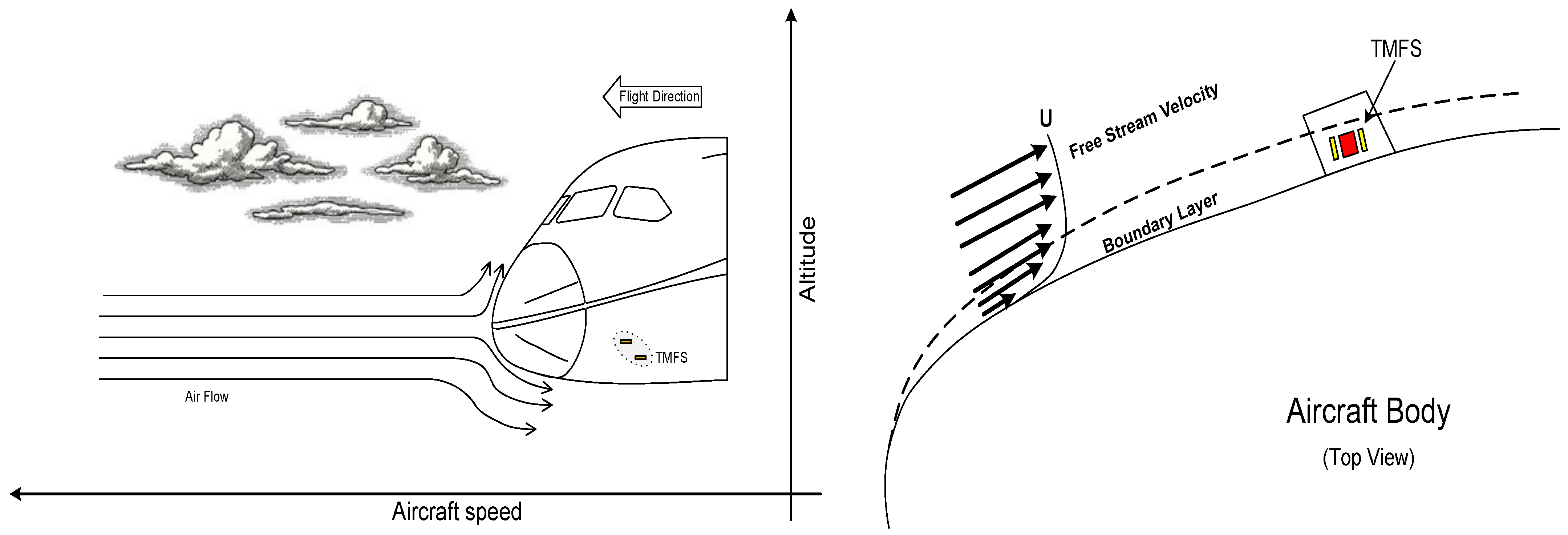
2. Proposed Calorimetric TMFS Application
3. Physics of the Application
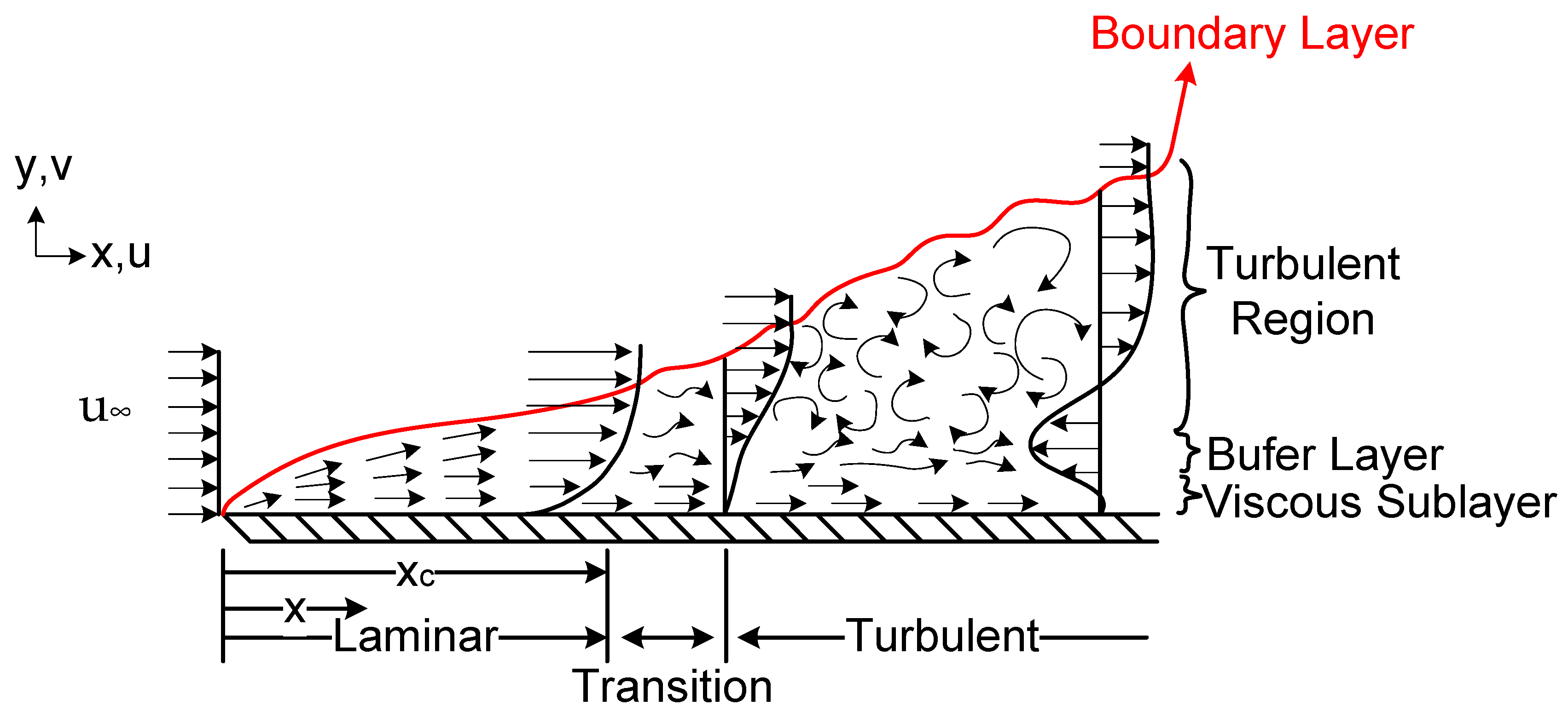
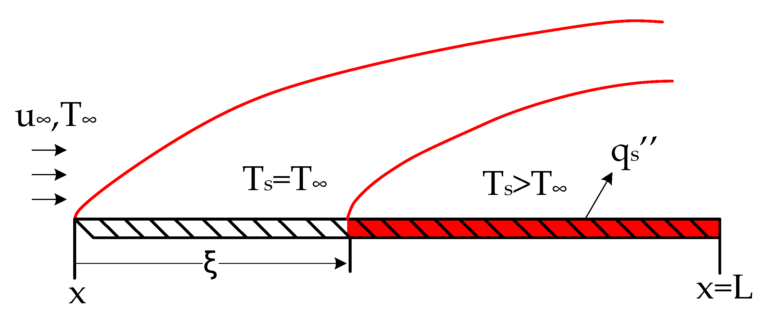
3.1. Heat Convection
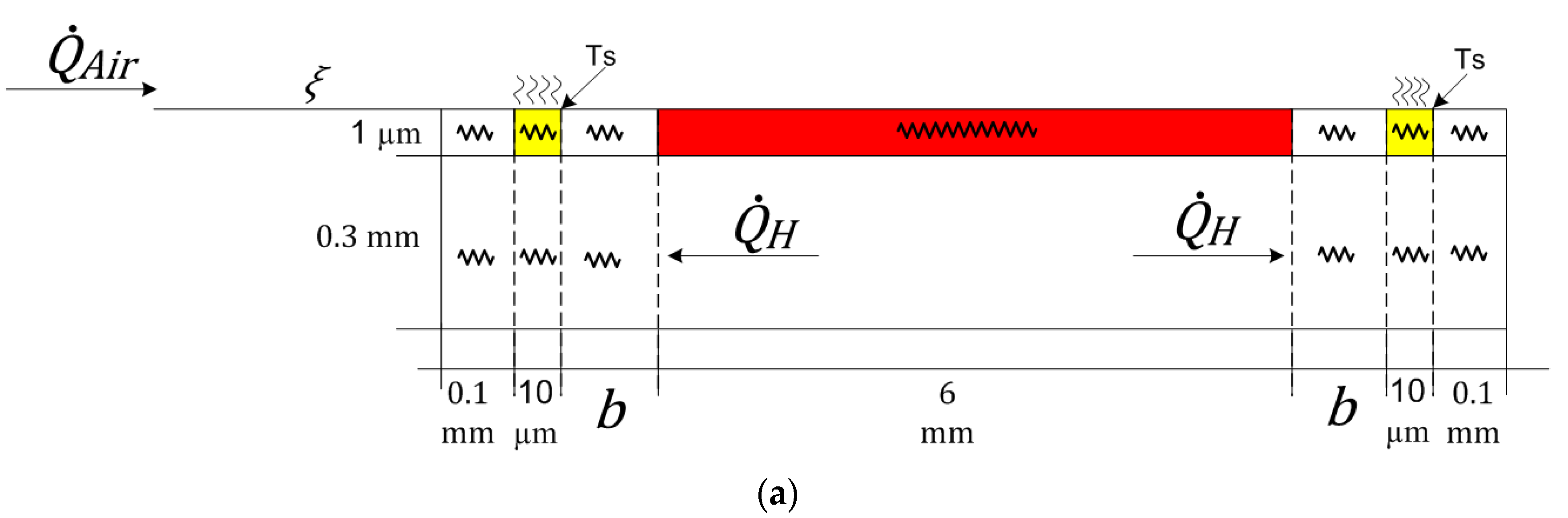
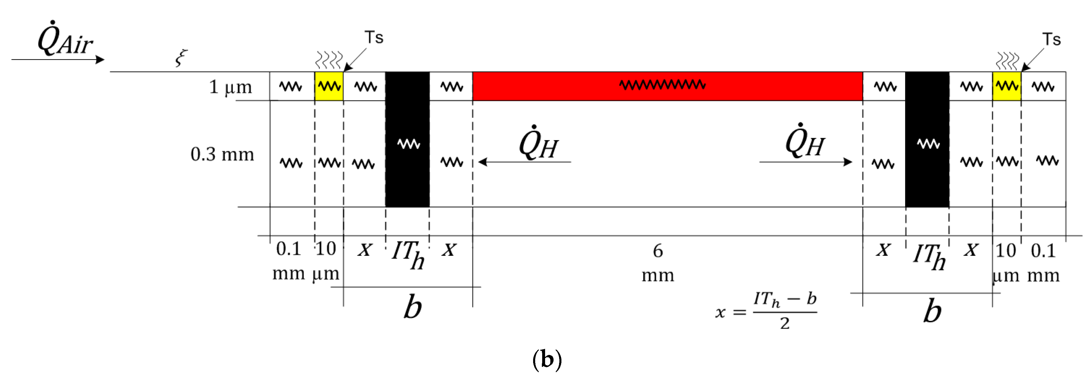
3.2. Heat Conduction
4. Materials and Methods
4.1. COMSOL Multiphysics
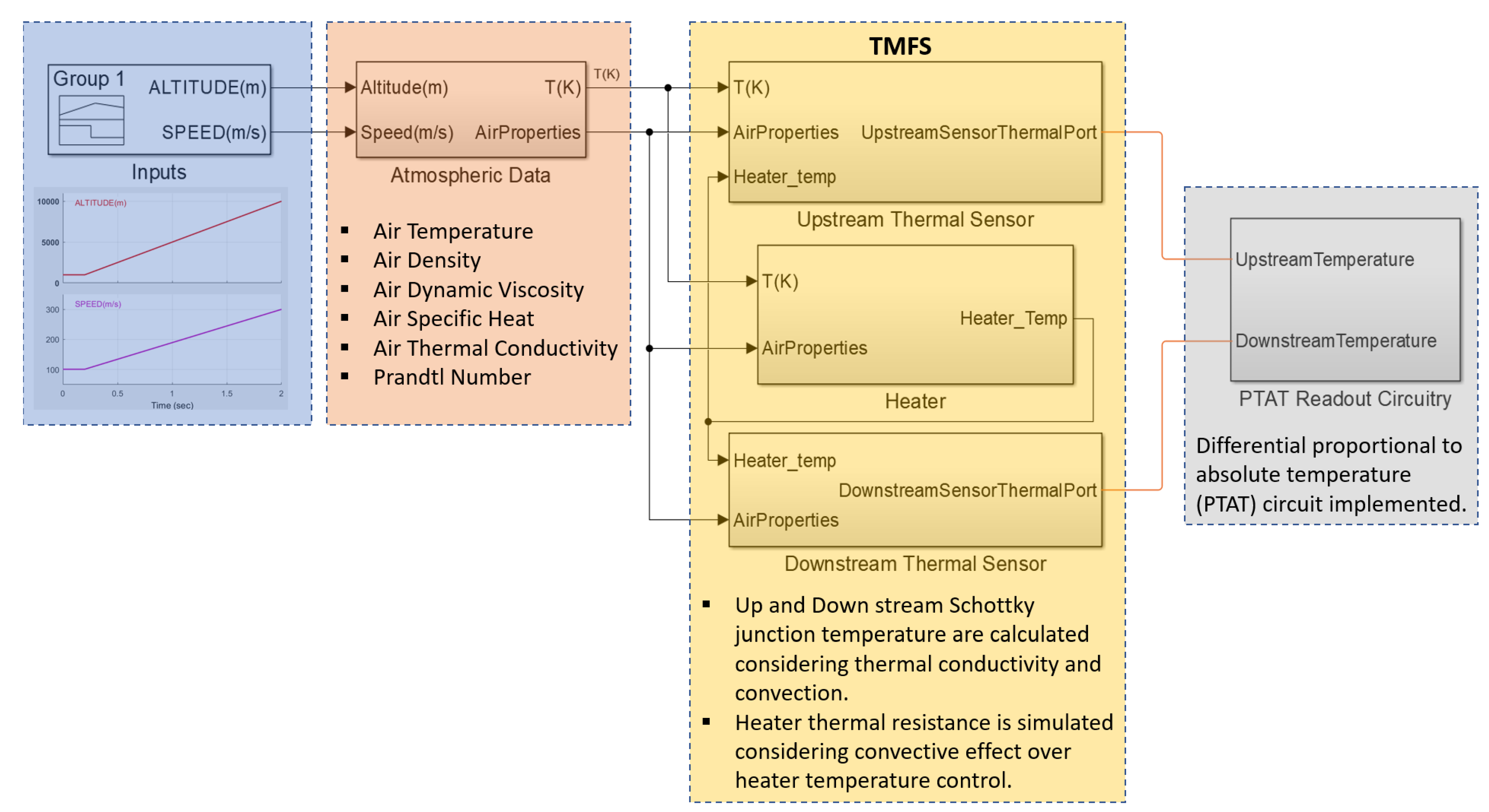
4.2. Simulink
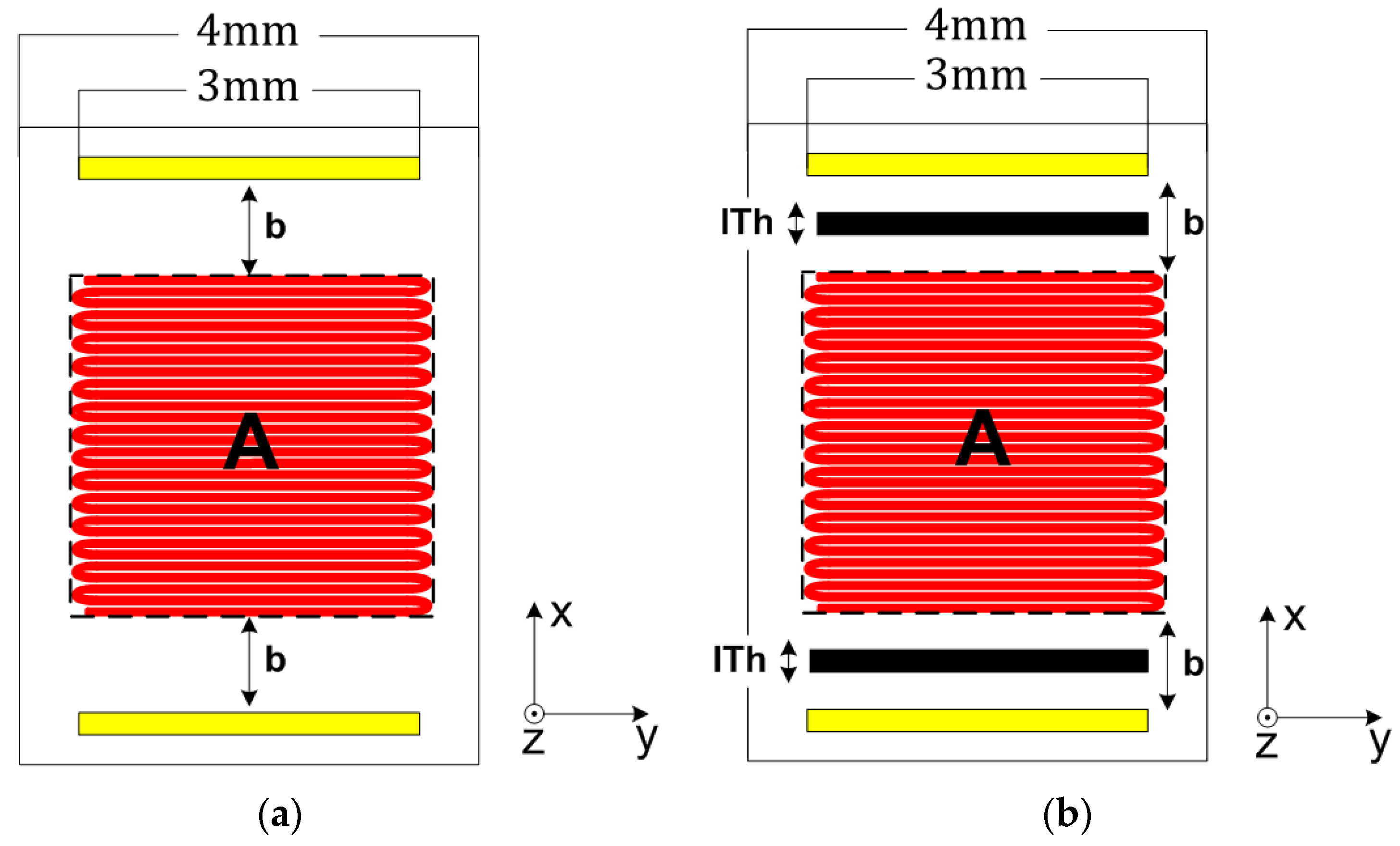
4.3. Calorimetric TMFS Fabrication Process
5. Results
5.1. COMSOL Multiphysics
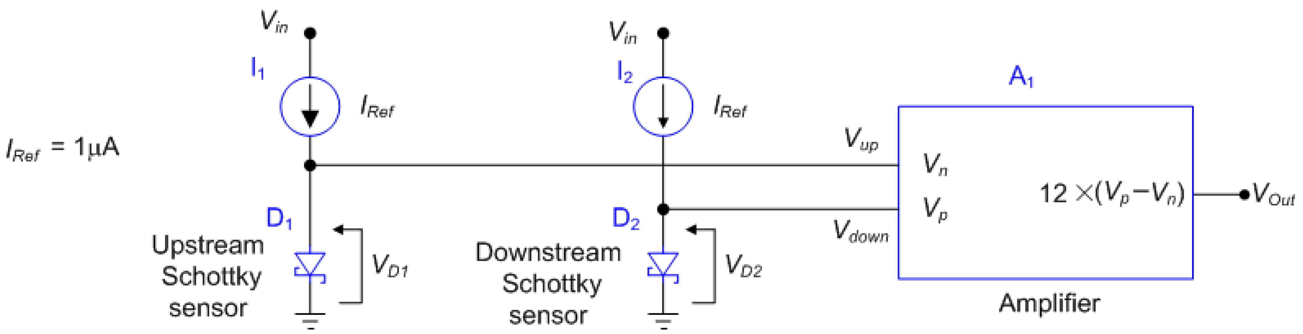
5.2. Simulink
6. Discussion
7. Conclusions
Author Contributions
Funding
Institutional Review Board Statement
Informed Consent Statement
Data Availability Statement
Acknowledgments
Conflicts of Interest
References
- Pratt, R.W. Flight Control Systems: Practical Issues in Design and Implementation; The Institution of Electrical Engineers and The American Institute of Aeronautics and Astronautics: Herts, UK, 2000. [Google Scholar]
- Nelson, R.C. Flight Stability and Automatic Control; McGraw-Hill Book Company: New York, NY, USA, 1989; ISBN 0-07-046218-6. [Google Scholar]
- Ali, A.; Souza, J.R.B.; Lisboa, K.M.; Cotta, R.M. Thermal analysis of heated pitot probes in atmospheric conditions of ice accretion. In Proceedings of the 23rd ABCM International Congress of Mechanical Engineering, COBEM, Rio de Janeiro, Brazil, 6–11 December 2015. [Google Scholar] [CrossRef]
- Bureau d’Enquêtes Et d’Analyses Pour La Sécurité De I’aviationcivile, Interim Report No 2 on the Accident on 1st June 2009 to the Airbus A330-203 Registered F-gzcp Operated by Air France Flight AF447 Rio de Janeiro-Paris. 2009. Available online: https://bea.aero/docspa/2009/f-cp090601.en/pdf/f-cp090601.en.pdf (accessed on 12 July 2018).
- Australian Transport Safety Bureau, In-Flight upset 154 Km West of Learmonth, WA 7 October 2008, VH-QPA, Airbus A330-303. 2008. Available online: https://www.atsb.gov.au/publications/investigation_reports/2008/aair/ao-2008-070.aspx (accessed on 12 July 2018).
- United Arab Emirates General Civil Aviation Authority, Serious Incident, Unreliable Airspeed Indication, Etihad Airways, A6-EHF, Airbus A340-600. 2013. Available online: https://www.gcaa.gov.ae/en/epublication/admin/iradmin/lists/incidents%20investigation%20reports/attachments/67/2013-2013%20-%20final%20report%20-%20aais%20case%20aifn-0005-2013%20-%20a6-ehf%20serious%20incident.pdf (accessed on 12 July 2018).
- Barbagallo, J. Pilot guide: Flight in ice condition. In FAA Advisory Circular Repository; [AC 91-74B]; Federal Aviation Administration: Washington, DC, USA, 2015. Available online: https://www.faa.gov/documentlibrary/media/advisory_circular/ac_91-74b.pdf (accessed on 23 August 2019).
- Tsao, T.; Jiang, F.; Miller, R.; Tai, Y.; Gupta, B.; Goodman, R.; Tung, S.; Ho, C. An integrated MEMS system for turbulent boundary layer control. In Proceedings of the International Solid State Sensors and Actuators Conference, Chicago, IL, USA, 19 June 1997; Volume 1, pp. 315–318. [Google Scholar] [CrossRef] [Green Version]
- Tung, S.; Maines, B.; Jiang, F.; Tsao, T. Development of a MEMS-Based Control System for Compressible Flow Separation. J. Microelectromechanical Syst. 2004, 13, 91–99. [Google Scholar] [CrossRef]
- Kumar, S.; Reynolds, W.; Kenny, T. MEMS based transducers for boundary layer control, Technical Digest. In Proceedings of the IEEE International MEMS 99 Conference, Orlando, FL, USA, 21 January 1999. [Google Scholar] [CrossRef]
- Sturm, H.; Dumstorff, G.; Busche, P.; Westermann, D.; Lang, W. Boundary layer separation and reattachment detection on airfoils by thermal flow sensors. Sensors 2012, 12, 14292–14306. [Google Scholar] [CrossRef] [PubMed] [Green Version]
- Mansoor, M.; Haneef, I.; Akhtar, S.; Rafiq, M.A.; Ali, S.Z.; Udrea, F. SOI CMOS multi-sensors MEMS chip for aerospace applications. In Proceedings of the IEEE Conference on Sensors, Valencia, Spain, 2–5 November 2014. [Google Scholar] [CrossRef]
- Leu, T.S.; Yu, J.M.; Miau, J.J.; Chen, S.J. MEMS flexible thermal flow sensors for measurement of unsteady flow above a pitching wind turbine blade. Exp. Therm. Fluid Sci. 2016, 77, 167–178. [Google Scholar] [CrossRef]
- Balakrishnan, V.; Phan, H.P.; Dinh, T.; Dao, D.V.; Nguyen, N.T. Thermal flow sensors for harsh environments. Sensors 2017, 17, 2061. [Google Scholar] [CrossRef] [PubMed] [Green Version]
- Que, R.; Zhu, R. Aircraft aerodynamic parameter detection using micro hot-film flow sensor array and BP neural network identification. Sensors 2012, 12, 10920–10929. [Google Scholar] [CrossRef] [Green Version]
- Lyons, C.; Friedberger, A.; Welser, W.; Muller, G.; Krotz, G.; Kassing, R. A high-speed mass flow sensor with heated silicon carbide bridges. In Proceedings of the MEMS 98, IEEE, Eleventh Annual International Workshop on Micro Electro Mechanical Systems. An Investigation of Micro Structures, Sensors, Actuators, Machines and Systems (Cat. No.98CH36176), Heidelberg, Germany, 25–29 January 1998; pp. 356–360. [Google Scholar] [CrossRef]
- Sun, J.; Qin, M.; Huang, Q. Flip-chip packaging for a two-dimensional thermal flow sensor using a copper pillar bump technology. IEEE Sens. J. 2007, 7, 990–995. [Google Scholar] [CrossRef]
- Kuo, J.T.W.; Yu, L.; Meng, E. Micromachined thermal flow sensors—A Review. Micromachines 2012, 3, 550–573. [Google Scholar] [CrossRef] [Green Version]
- Billat, S.; Storz, M.; Ashauer, H.; Hedrich, F.; Kattinger, G.; Lust, L.; Ashauer, M.; Zengerle, R. Thermal flow sensors for harsh environment applications. Procedia Chem. 2009, 1, 1459–1462. [Google Scholar] [CrossRef] [Green Version]
- Lange, P.; Weiss, M.; Warnat, S. Characteristics of a micro-mechanical thermal flow sensor based on a two hot wires principle with constant temperature operation in a small channel. J. Micromech. Microeng. 2014, 24, 125005. [Google Scholar] [CrossRef]
- Jiang, F.; Lee, G.B.; Tai, Y.C.; Ho, C.M. A flexible micromachine-based shear-stress sensor array and its application to separation-point detection. Sens. Actuators A Phys. 2000, 79, 194–203. [Google Scholar] [CrossRef]
- Cerimovic, S.; Talic, A.; Beigelbeck, R.; Sauter, T.; Kohl, F.; Schalko, J.; Keplinger, F. A novel calorimetric flow sensor implementation based on thermal sigma-delta modulation. In Proceedings of the SENSORS, 2009 IEEE, Christchurch, New Zealand, 25–28 October 2009; pp. 1923–1926. [Google Scholar] [CrossRef]
- Mehmood, Z.; Haneef, I.; Ali, S.Z.; Udrea, F. Sensitivity enhancement of silicon-on-insulator CMOS MEMS thermal hot-film flow sensors by minimizing membrane conductive heat losses. Sensors 2019, 19, 1860. [Google Scholar] [CrossRef] [PubMed] [Green Version]
- Glatzl, T.; Beigelbeck, R.; Cerimovic, S.; Steiner, H.; Wenig, F.; Sauter, T.; Treytl, A.; Keplinger, F. A thermal flow sensor based on printed circuit technology in constant temperature mode for various fluids. Sensors 2019, 19, 1065. [Google Scholar] [CrossRef] [Green Version]
- Kaltsas, G.; Nassiopoulos, A.A.; Nassiopoulou, A.G. Characterization of a silicon thermal gas-flow sensor with porous silicon thermal isolation. IEEE Sens. J. 2002, 2, 463–475. [Google Scholar] [CrossRef]
- Petropoulos, A.; Kaltsas, G. Study and evaluation of a PCB-MEMS liquid microflow sensor. Sensors 2010, 10, 8981–9001. [Google Scholar] [CrossRef] [PubMed] [Green Version]
- Kim, T.H.; Dong-Kwon, K.; Sung, J.K. Study of the sensitivity of a thermal flow sensor. Int. J. Heat Mass Transf. 2009, 52, 7–8. [Google Scholar] [CrossRef]
- Wang, Y.; Dai, W.; Wu, Y.; Guo, Y.; Xu, R.; Yan, B.; Xu, Y. A bendable microwave GaN HEMT on CVD Parylene-C substrate. In Proceedings of the IEEE MTT-S International Conference on Numerical Electromagnetic and Multiphysics Modeling and Optimization (NEMO), Hangzhou, China, 7–9 December 2020. [Google Scholar]
- Li, L.; Mason, A.J. Post-CMOS parylene packaging for on-chip biosensor arrays. In Proceedings of the IEEE Sensors Conference, Waikoloa, HI, USA, 1–4 November 2010. [Google Scholar]
- Mayer, F.; Paul, O.; Baltes, H. Influence of Design Geometry and Packaging on the response of thermal CMOS flow sensors. In Proceedings of the International Solid-State Sensors and Actuators Conference—TRANSDUCERS, Stockholm, Sweden, 25–29 June 1995. [Google Scholar]
- Bruschi, P.; Piotto, M. Design issues for low power integrated thermal flow sensors with ultra-wide dynamic range and low insertion loss. Micromachines 2012, 3, 295–314. [Google Scholar] [CrossRef] [Green Version]
- Hoeneisen, B.; Mead, C.A. Power Schottky diode design and comparison with the junction diode. Solid-State Electron. 1971, 14, 1225–1236. [Google Scholar] [CrossRef]
- Pascu, R.; Pristavu, G.; Brezeanu, G.; Draghici, F.; Godignon, P.; Romanitan, C.; Matei, S.; Adrian, T. 60–700 K CTAT and PTAT temperature sensors with 4H-SiC Schottky diodes. Sensors 2021, 21, 942. [Google Scholar] [CrossRef]
- Mitra, J.; Feng, L.; Penate, L.; Dawson, P. An alternative methodology in Schottky diode physics. J. Appl. Phys. 2015, 117, 244501. [Google Scholar] [CrossRef]
- Josan, I.; Boianceanu, C.; Brezeanu, G.; Obreja, V.; Avram, M.; Puscasu, D.; Ioncea, A. Extreme environment temperature sensor based on silicon carbide Schottky Diode. In Proceedings of the International Semiconductor Conference, Sinaia, Romania, 12–14 October 2009. [Google Scholar] [CrossRef]
- Zhang, N.; Pisano, A. Harsh environment temperature sensor based on 4H-Silicon carbide PN diode. In Proceedings of the International Conference on Solid State Sensors and Actuators (TRANSDUCERS), Barcelona, Spain, 16–20 June 2013. [Google Scholar] [CrossRef]
- Rao, S.; Pangallo, G.; Pezzimenti, F.; Della Corte, F. High-performance temperature sensor based on 4H-SiC Schottky diodes. IEEE Electron Device Lett. 2015, 36, 720–722. [Google Scholar] [CrossRef]
- White, F.M. Viscous Fluid Flow, 3rd ed.; McGraw-Hill Book Company: New York, NY, USA, 2006; ISBN 007-124493-X. [Google Scholar]
- Bergman, T.L.; Lavine, A.S.; Incropera, F.P.; Dewitt, D.P. Fundamentals of Heat and Mass Transfer, 7th ed.; John Willey & Sons: Hoboken, NJ, USA, 2011; ISBN 13 978-0470-50197-9. [Google Scholar]
- Alam, J.M.; Walsh, R.P.; Hossain, M.A.; Rose, A.M. A computational methodology for two-dimensional fluid flows. Int. J. Numer. Meth. Fluids 2014, 75, 835–859. [Google Scholar] [CrossRef]
- Alizard, F.; Robinet, J.C. Modeling of optimal perturbations in flat plate boundary layer using global modes: Benefits and limits. Theory Comput. Fluid Dyn. 2011, 25, 147–165. [Google Scholar] [CrossRef]
- Cardarelli, F. Materials Handbook: A Concise Desktop Reference; Springer: Berlin/Heidelberg, Germany, 2005; ISBN 978-1-84628-668-1. [Google Scholar]
- ISA. Manual of the ICAO Standard Atmosphere. International Civil Aviation Organization. 1993. Available online: http://code7700.com/pdfs/icao/icao_doc_7488_standard_atmosphere.pdf (accessed on 9 May 2017).
- Ribeiro, L.C.; Korsa, M.T.; Saotome, O.; Adam, J.; Hansen, R.M.O. Design of a micro-machined flow sensor for aircraft air data systems application: Mechanical considerations. In Proceedings of the International Conference on Microelectronics and Microsystems Technology ICMMT, New York, NY, USA, 10–11 December 2020. [Google Scholar]
- Krasnov, V.A.; Shutov, S.V.; Yerochin, S.Y.; Demenskyi, O.M. High Temperature operation limit assessment for 4H-SiC schottky diode-based extreme temperature sensors. IEEE Sens. J. 2019, 19, 1640–1644. [Google Scholar] [CrossRef]
- Racka-Szmidt, K.; Stonio, B.; Zelazko, J.; Filipiak, M.; Sochacki, M. A review: Inductively coupled plasma reactive ion etching of silicon carbide. Materials 2022, 15, 123. [Google Scholar] [CrossRef]


| Property | Unit | Substrate (SiC) | Insulation (Parylene N) | Heater (W) | Thermal Sensor (Au) |
|---|---|---|---|---|---|
| Electrical Resistivity | Ωm @ 20 °C | 10 | - | 5.65 × 10⁻⁸ | 2.44 × 10⁻⁸ |
| Thermal Conductivity | W/m—K | 114 | 0.126 | 174 | 300 |
| Young’s Module | Nmm2 | 4.15 × 10⁵ | - | 4.11 × 10⁵ | 79 × 103 |
| Poisson’s Ratio | N/A | 0.16 | - | 0.280 | 0.42 |
| Density | gcm−3 @ 25 °C | 3.16 | 1.11 | 19.3 | 19.32 |
| Melting Point | °C | 2830 | - | 3687 | 1064 |
| Specific Heat Capacity | J/g-°C | 0.670 | 1.3 | 0.134 | 0.133 |
| Property | Unit | Value |
|---|---|---|
| Dynamic Viscosity | μPa.s | 17.606 |
| Sound Speed | m/s | 336.766 |
| Kinematic Viscosity | μm2/s | 15.705 |
| Thermal Conductivity | W/m·K | 0.024874 |
| Altitude | m | 1000 |
| Temperature | K | 282.207 |
| Pressure | hPa | 90,813 |
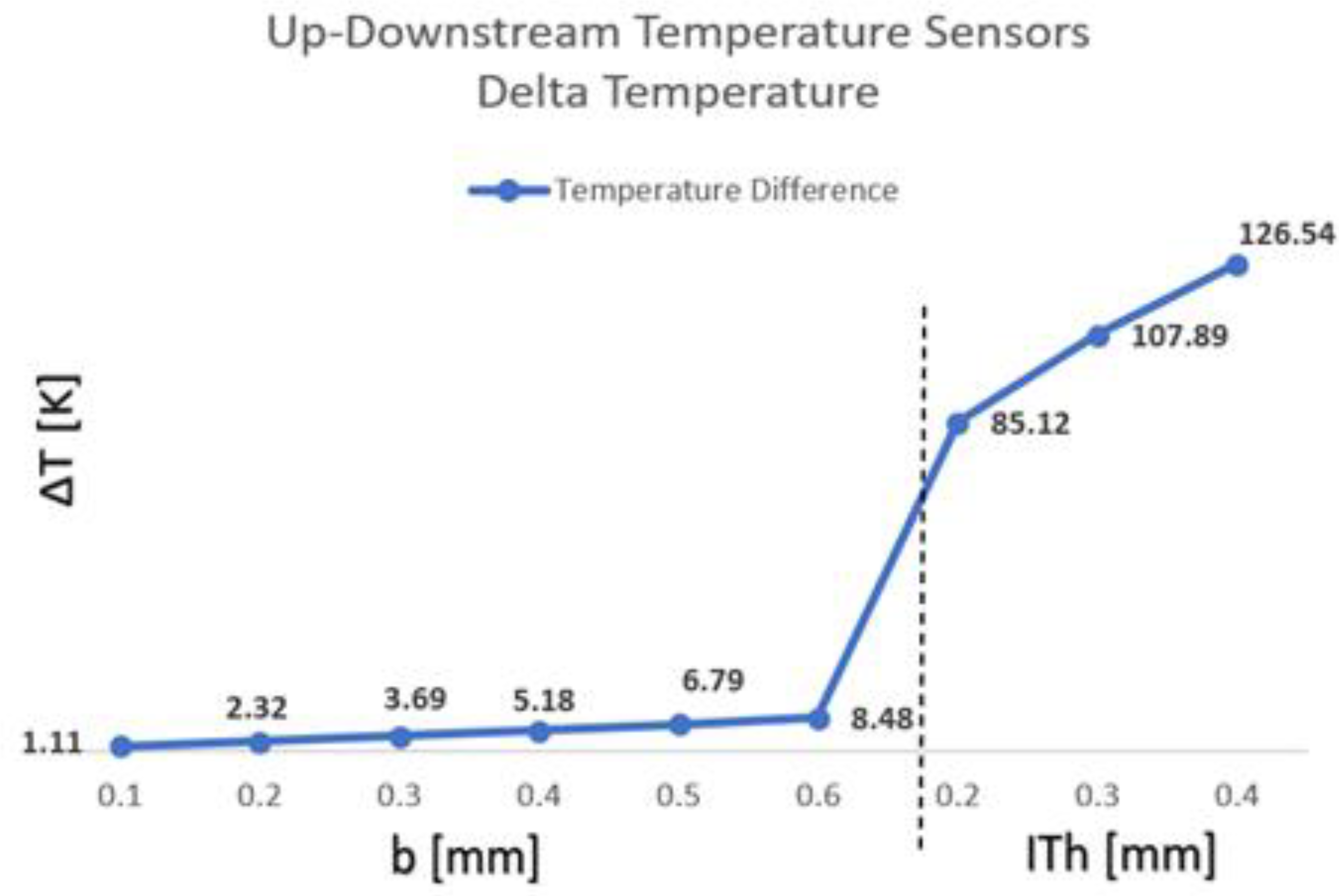
| 0.1 | 0.2 | 0.3 | 0.4 | 0.5 | 0.6 | 0.6/0.2 | 0.6/0.3 | 0.6/0.4 | |
|---|---|---|---|---|---|---|---|---|---|
| Domain | 1,427,329 | 1,464,080 | 1,500,454 | 1,535,496 | 1,571,820 | 1,607,178 | 1,602,022 | 1,602,876 | 1,601,974 |
| Boundary | 29,378 | 29,967 | 30,549 | 31,126 | 31,698 | 32,266 | 32,520 | 32,526 | 32,540 |
| Minimum Quality | 0.4875 | 0.4485 | 0.4491 | 0.4386 | 0.4748 | 0.4484 | 0.4484 | 0.4484 | 0.4484 |
| Error in Kelvin (%) | ||||
|---|---|---|---|---|
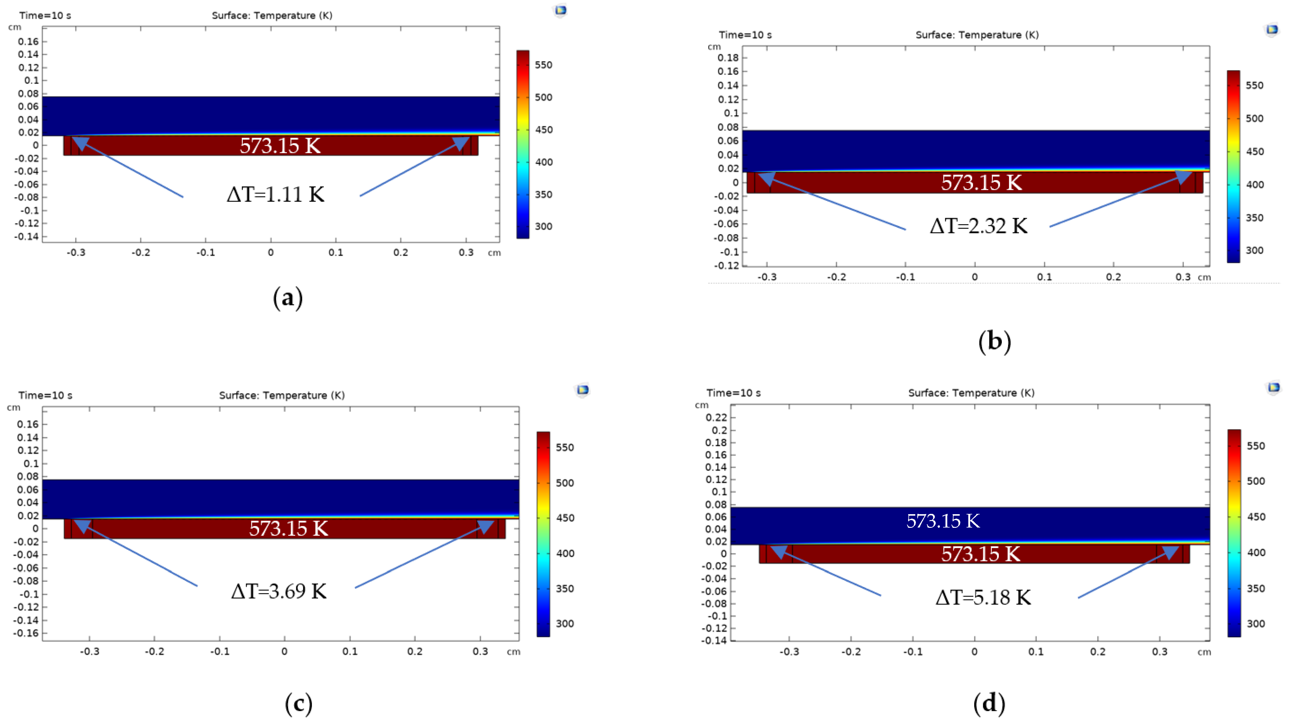
| 0.1 | 0 | 1.1 | 2.6 | 1.5 (58%) |
| 0.2 | 0 | 2.32 | 3.5 | 1.18 (34%) |
| 0.3 | 0 | 3.69 | 4.4 | 0.71 (16%) |
| 0.4 | 0 | 5.18 | 5.4 | 0.22 (4%) |
| 0.5 | 0 | 6.79 | 6.4 | 0.39 (6%) |
| 0.6 | 0 | 8.48 | 7.5 | 0.98 (13%) |
| 0.6 | 0.1 | 85.12 | 87.5 | 2.38 (3%) |
| 0.6 | 0.2 | 107.89 | 114.9 | 7.01 (6%) |
| 0.6 | 0.3 | 126.54 | 135 | 8.46 (6%) |
Publisher’s Note: MDPI stays neutral with regard to jurisdictional claims in published maps and institutional affiliations. |
© 2022 by the authors. Licensee MDPI, Basel, Switzerland. This article is an open access article distributed under the terms and conditions of the Creative Commons Attribution (CC BY) license (https://creativecommons.org/licenses/by/4.0/).
Share and Cite
Ribeiro, L.; Saotome, O.; d’Amore, R.; de Oliveira Hansen, R. High-Speed and High-Temperature Calorimetric Solid-State Thermal Mass Flow Sensor for Aerospace Application: A Sensitivity Analysis. Sensors 2022, 22, 3484. https://doi.org/10.3390/s22093484
Ribeiro L, Saotome O, d’Amore R, de Oliveira Hansen R. High-Speed and High-Temperature Calorimetric Solid-State Thermal Mass Flow Sensor for Aerospace Application: A Sensitivity Analysis. Sensors. 2022; 22(9):3484. https://doi.org/10.3390/s22093484
Chicago/Turabian StyleRibeiro, Lucas, Osamu Saotome, Roberto d’Amore, and Roana de Oliveira Hansen. 2022. "High-Speed and High-Temperature Calorimetric Solid-State Thermal Mass Flow Sensor for Aerospace Application: A Sensitivity Analysis" Sensors 22, no. 9: 3484. https://doi.org/10.3390/s22093484