

The Best of Both Worlds: A Framework for Combining Degradation Prediction with High Performance Super-Resolution Networks

 , , , , and
Abstract
1. Introduction
- A framework for the integration of degradation prediction systems into SOTA non-blind SR networks.
- A comprehensive evaluation of different methods for the insertion of blur kernel metadata into CNN SR networks. Specifically, our results show that simple metadata insertion blocks ( such as MA) can match the performance of more complex metadata insertion systems when used in conjunction with large SR networks.
- Blind SR results using a combination of non-blind SR networks and SOTA degradation prediction systems. These hybrid models show improved performance over both the original SR network and the original blind prediction system.
- A thorough comparison of unsupervised, semi-supervised and supervised degradation prediction methods for both simple and complex degradation pipelines.
- The successful application of combined (i) blind degradation prediction and (ii) SR of images, degraded with a complex pipeline involving multiple types of noise, blurring and compression that is more reflective of real-world applications than considered by most SISR approaches.
2. Related Work
2.1. Degradation Models
2.2. Non-Blind SR Methods
2.3. Blind SR Methods
2.3.1. Approaches Utilising Supplementary Attributes for SR
2.3.2. Iterative Kernel Estimation Methods
2.3.3. Training SR Models on a Single Image
2.3.4. Implicit Degradation Modelling
2.3.5. Contrastive Learning
2.3.6. Other Methodologies
2.4. Conclusions
3. Methodology
3.1. Degradation Model
3.2. Framework for Combining SR Models with a Blind Predictor
3.3. Metadata Insertion Block
- SRMD-style [39] (Figure 2A): An early adopter of metadata insertion in SR, the SRMD technique involves the transformation of vectors as additional pseudo-image channels. Each element of the input degradation vector is expanded (by repeated tiling) into a 2D array, with the same dimensions as the input LR image. These pseudo-channels are then fed into the network along with the real image data, ensuring that all convolutional filters in the first layer have access to the degradation information. Other variants of this method, which include directly combining the pseudo-channels with CNN feature maps, have also been proposed [23]. The original SRMD network used this method for Principal Component Analysis (PCA)-reduced blur kernels and noise values. In our work, we extended this methodology to all degradation vectors considered.
- MA [26] (Figure 2B): MA is a trainable channel attention block which was proposed as a way to upgrade any CNN-based SR network with metadata information. Its functionality is simple—an input vector is stretched to the same size as the number of feature maps within a target CNN network using two fully-connected layers. Each vector element is normalised to lie in the closed interval and then applied to selectively amplify its corresponding CNN feature map. MA was previously applied for PCA-reduced blur kernels and compression quality factors only. We extended this mechanism to all degradation parameters considered, by combining them into an input vector which is then fed into the MA block. The fully-connected layer sizes were then expanded as necessary to accommodate the input vector.
- SFT [22] (Figure 2C): The SFT block is based on the SRMD concept but with additional layers of complexity. The input vector is also stretched into pseudo-image channels, but these are added to the feature maps within the network rather than the actual original image channels. This combination of feature maps and pseudo-channels are then fed into two separate convolutional pathways, one of which is multiplied with the original feature maps and the other added on at the end of the block. This mechanism is the largest (in terms of parameter count due to the number of convolutional layers) of those considered in this paper. As with SRMD, this method has only been applied for blur kernel and noise parameter values, and we again extended the basic concept to incorporate all degradation vectors considered.
- Degradation-aware (DA) block [24] (Figure 2D): The DA block was proposed in combination with a contrastive-based blind SR mechanism for predicting blur kernel degradations. It uses two parallel pathways, one of which amplifies feature maps in a manner similar to MA, while the other explicitly transforms vector metadata into a 3D kernel, which is applied on the network feature maps. This architecture is highly specialised to kernel-like degradation vectors, but could still be applicable for general degradation parameters given its dual pathways. We extended the DA block to all degradation vectors as we did with the MA system.
- Degradation-Guided Feature Modulation Block (DGFMB) [25] (Figure 2E): This block was conceived as part of another contrastive-based network, again intended for blur and noise degradations. The main difference here is that the network feature maps are first reduced into vectors and concatenated with the degradation metadata in this form, rather than in image space. Once the vectors are concatenated, a similar mechanism to MA is used to selectively amplify the output network feature maps. As before, we extended this mechanism to other degradation parameters by combining these into an input vector.
3.4. Degradation Prediction—Iterative Mechanism
3.5. Degradation Prediction—Contrastive Learning
3.5.1. MoCo—Unsupervised Mechanism
- Two identical encoders are instantiated. One acts as the ‘query’ encoder and the other as the ‘key’ encoder. The query encoder is updated directly via backpropagation from computed loss, while the key encoder is updated through a momentum mechanism from the query encoder.
- The encoders are each directed to generate a degradation vector from one separate square patch per LR image, as shown on the right-hand side of Figure 3A. The query encoder vector is considered as the reference for loss calculation, while the key encoder vector generated from the second patch acts as a positive sample. The training objective is to drive the query vector to become more similar to the positive sample vector, while simultaneously repelling the query vector away from encodings generated from all other LR images (negative samples).
- Negative samples are generated by placing previous key encoder vectors from distinct LR images into a queue. With both positive and negative encoded vectors available, an InfoNCE-based [75] loss function can be applied:where and are the query and key encoders, respectively, is the first patch from the ith image in a batch (batch size B), is the jth entry of the queue of size and is a constant temperature scalar. With this loss function, the query encoder is updated to simultaneously move its prediction closer to the positive encoding, and farther away from the negative set of encodings. This push-pull effect is depicted by the coloured dotted lines within the MoCo box in Figure 3A. This loss should enable the encoder to distinguish between the different degradations present in the positive and negative samples.
3.5.2. SupMoCo—Semi-Supervised Mechanism
- Blur kernel type
- Blur kernel size; either low/high, which we refer to as double precision (2 clusters per parameter), or low/medium/high, which we refer to as triple precision (3 clusters per parameter), classification.
- Noise type
- Noise magnitude (either a double or triple precision classification)
- Compression type
- Compression magnitude (either a double or triple precision classification)
3.5.3. WeakCon—Semi-Supervised Mechanism
3.5.4. Direct Regression Attachment
3.6. Extensions to Degradation Prediction
4. Experiments & Results
4.1. Implementation Details
4.1.1. Datasets and Degradations
- Simple pipeline (blurring and downsampling): For our metadata insertion screening and blind SR comparison, we used a degradation set of just Gaussian blurring and bicubic downsampling corresponding to the ‘classical’ degradation model described in Equation (2). Apart from minimising confounding factors, this allowed us to make direct comparisons with pre-trained models provided by the authors of other blind SR networks. For all scenarios, we used only 21 × 21 isotropic Gaussian kernels with a random width () in the range (as recommended in [16]), and ×4 bicubic downsampling. The parameter was then normalised to the closed interval before it was passed to the models.
- Complex pipeline: In our extended blind SR training schemes, we used a full degradation pipeline as specified in Equation (3), i.e., sequential blurring, downsampling, noise addition and compression. For each operation in the pipeline, a configuration was randomly (from a uniform distribution) selected from the following list:
- −
- Blurring: As proposed in [16], we sampled blurring from a total of 7 different kernel shapes: iso/anisotropic Gaussian, iso/anisotropic generalised Gaussian, iso/anisotropic plateau, and sinc. Kernel values (both vertical and horizontal) were sampled from the range , kernel rotation ranged from to (all possible rotations) and the shape parameter ranged from for both generalised Gaussian and plateau kernels. For sinc kernels, we randomly selected the cutoff frequency from the range . All kernels were set to a size of 21 × 21 and, in each instance, the blur kernel shape was randomly selected, with equal probability, from the 7 available options. For a full exposition on the selection of each type of kernel, please refer to [16].
- −
- Downsampling: As in the initial model screening, we again retained ×4 bicubic downsampling for all LR images.
- −
- Noise addition: Again following [16], we injected noise using one of two different mechanisms, namely Gaussian (signal independent read noise) and Poisson (signal dependent shot noise). Additionally, the noise was either independently added to each colour channel (colour noise), or applied to each channel in an identical manner (grey noise). The Gaussian and Poisson mechanisms were randomly applied with equal probability, grey noise was selected with a probability of 0.4, and the Gaussian/Poisson sigma/scale values were randomly sampled from the ranges and , respectively.
- −
- Compression: We increased the complexity of compression used in previous works by randomly selecting from either JPEG or JM H.264 (version 19) [76] compression at runtime. For JPEG, a quality value was randomly selected from the range (following [16]). For JM H.264, images were compressed as single-frame YUV files where a random I-slice Quantization Parameter (QPI) was selected from the range , as discussed in [26].
4.1.2. Model Implementation, Training and Validation
- Non-blind SR model training: For non-blind model training, we initialised the networks with the hyperparameters as recommended by their authors, unless otherwise specified. All models were trained from scratch on LR–HR pairs generated from the DIV2K and Flickr2K datasets using either the simple or complex pipelines. For the simple pipeline, one LR image was generated from each HR image. For the complex pipeline, five LR images were generated per HR image to improve the diversity of degradations available. In both cases, the LR image set was generated once and used to train all models. All simple pipeline networks were trained for 1000 epochs, whereas the complex pipeline networks were trained for 200 epochs to ensure fair comparisons (since each epoch contains 5 times as many samples as in the simple case). This training duration (in epochs) was chosen as a compromise between obtaining meaningful results and keeping the total training time low.For both pipelines, training was carried out on 64 × 64 LR patches. The Adam [87] optimiser was used. Variations in batch size and learning rate scheduling were made for specific models as necessary in order to ensure training stability and limit Graphical Processing Unit (GPU) memory requirements. The configurations for the non-blind SR models tested are as follows:
- −
- RCAN [8] and HAN [10]: We selected RCAN to act as our baseline model as a compromise between SR performance and architectural simplicity. To push performance boundaries further, we also trained and tested HAN as a representative SOTA pixel-quality CNN-based SR network. For these models, the batch size was set to 8 in most cases, and a cosine annealing scheduler [88] was used with a warm restart after every 125,000 iterations and an initial learning rate of 1 × 10⁻⁴. Training was driven solely by the L1 loss function which compares the SR image with the target HR image. After training, the epoch checkpoint with the highest validation PSNR was selected for final testing.
- −
- Real-ESRGAN [16]: We selected Real-ESRGAN as a representative SOTA perceptual quality SR model. The same scheme described for the original implementation was used to train this network. This involved two phases: (i) a pre-training stage where the generator was trained with just an L1 loss, and (ii) a multi-loss stage where a discriminator and VGG perceptual loss network were introduced (further details are provided in [16]). We pre-trained the model for 715 and 150 epochs (which match the pretrain:GAN ratio as originally proposed in [16]) for the simple and complex pipelines, respectively. In both cases, the pre-training optimiser learning rate was fixed at , while the multi-loss stage involved a fixed learning rate of . A batch size of 8 was used in all cases. After training, the model checkpoint with the lowest validation LPIPS score in the last 10% of epochs was selected for testing.
- −
- ELAN [13]: We also conducted a number of experiments with ELAN, a SOTA transformer-based model. For this network a batch size of 8 and a constant learning rate of were used in all cases. As with RCAN and HAN, the L1 loss was used to drive training and the epoch checkpoint with the highest validation PSNR was selected for final testing.
- Iterative Blind SR: Since the DAN iterative scheme requires the SR image to improve its degradation estimate, the predictor model needs to be trained simultaneously with the SR model. We used the same CNN-based predictor network described in DANv1 [23] for our models and fixed the iteration count to four in all cases (matching the implementation as described in [23]). We coupled this predictor with our non-blind SR models using the framework described in Section 3.2. We trained all DAN models by optimising for the SR L1 loss (identical to the non-blind models) and an additional L1 loss component comparing the prediction and ground-truth vectors. Target vectors varied according to the pipeline, the details of each are provided in their respective results sections. For each specific model architecture, the hyperparameters and validation selection criteria were all set to be identical to that of the base, non-blind model. The batch size for all models was adjusted to 4 due to the increased GPU memory requirements needed for the iterative training scheme. Accordingly, whenever a warm restart scheduler was used, the restart point was adjusted to 250,000 iterations (to maintain the same total number of iterations as performed by the other models that utilised a batch size of 8 for 125,000 iterations).Additionally, we also trained the original DANv1 model from scratch, using the same hyperparameters from [23] and the same validation scheme as the other DAN models. The batch size was also fixed to 4 in all cases.
- Contrastive Learning: We used the same encoder from [24] for most of our contrastive learning schemes. This encoder consists of a convolutional core connected to a set of three fully-connected layers. During training, we used the output of the fully-connected layers (Q) to calculate loss values (i.e., and in Section 5) and update the encoder weights, following [24]. Before coupling the encoder with an SR network, we first pre-trained the encoder directly. For this pre-training, the batch size was set to 32 and data was generated online, i.e., each LR image was synthesised on the fly at runtime. All encoders were trained with a constant learning rate of , a patch size of 64 × 64 and the Adam optimiser. The encoders were trained until the loss started to plateau and t-Distributed Stochastic Neighbour Embedding (t-SNE) clustering of degradations generated on a validation set composed of 400 images from CelebA [89] and BSDS200 [81] was clearly visible (more details on this process are provided in Section 4.3.1). In all cases, the temperature hyperparameter, momentum value, queue length, and encoder output vector size were set to 0.07, 0.999, 8192 and 256, respectively, (matching the models from [24]).After pre-training, each encoder was coupled to non-blind SR networks using the framework discussed in Section 3.2. For standard encoders, the encoding (i.e., the output from the convolutional core that bypasses the fully-connected layers) is typically fed into metadata insertion blocks directly, unless specified. For encoders with a regression component (see Figure 2B), the dropdown output is fed to the metadata insertion block instead of the encoding. The combined encoder + SR network was then trained using the same dataset and hyperparameters as the non-blind case. The encoder weights were frozen and no gradients were generated for the encoding at runtime, unless specified.
4.2. Metadata Insertion Block Testing
4.3. Blur Kernel Degradation Prediction
4.3.1. Contrastive Learning
4.3.2. Regression Analysis
4.4. Blind SR on Simple Pipeline
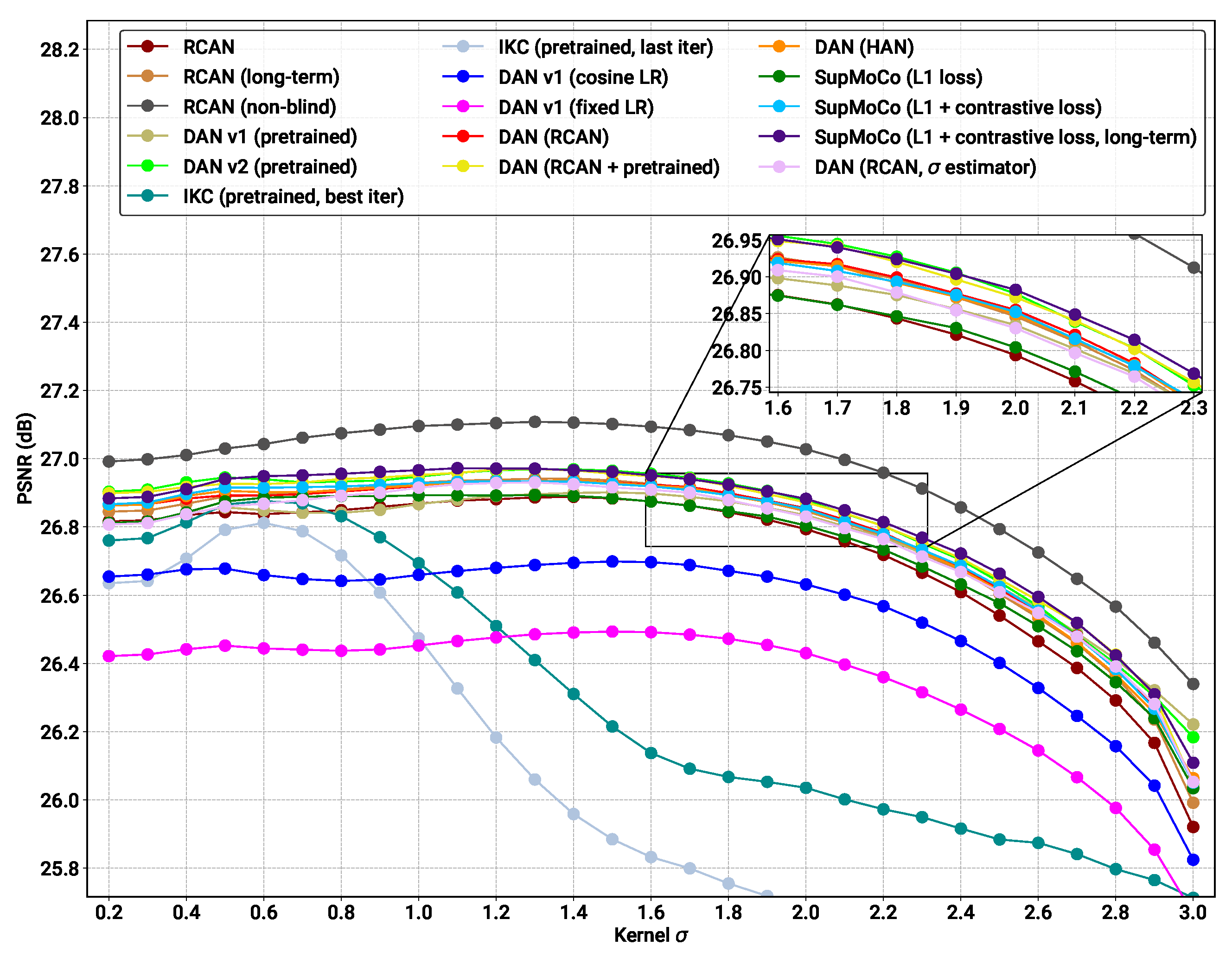
- Pretrained models: We provide the results for the pretrained models evaluated in Figure 7B, along with the results for the pretrained DASR [24], a blind SR model with a MoCo-based contrastive encoder. The DAN models have the best results in most cases (with DANv2 having the best performance overall). For IKC, another iterative model, we present two sets of metrics: IKC (pretrained-best-iter) shows the results obtained when selecting the best image from all SR output iterations (7 in total), as is the implementation in the official IKC codebase. IKC (pretrained-last-iter) shows the results obtained when selecting the image from the last iteration (as is done for the DAN models). The former method produces the best results (even surpassing DAN in some cases), but cannot be applied in true blind scenarios where a reference HR image is not available.
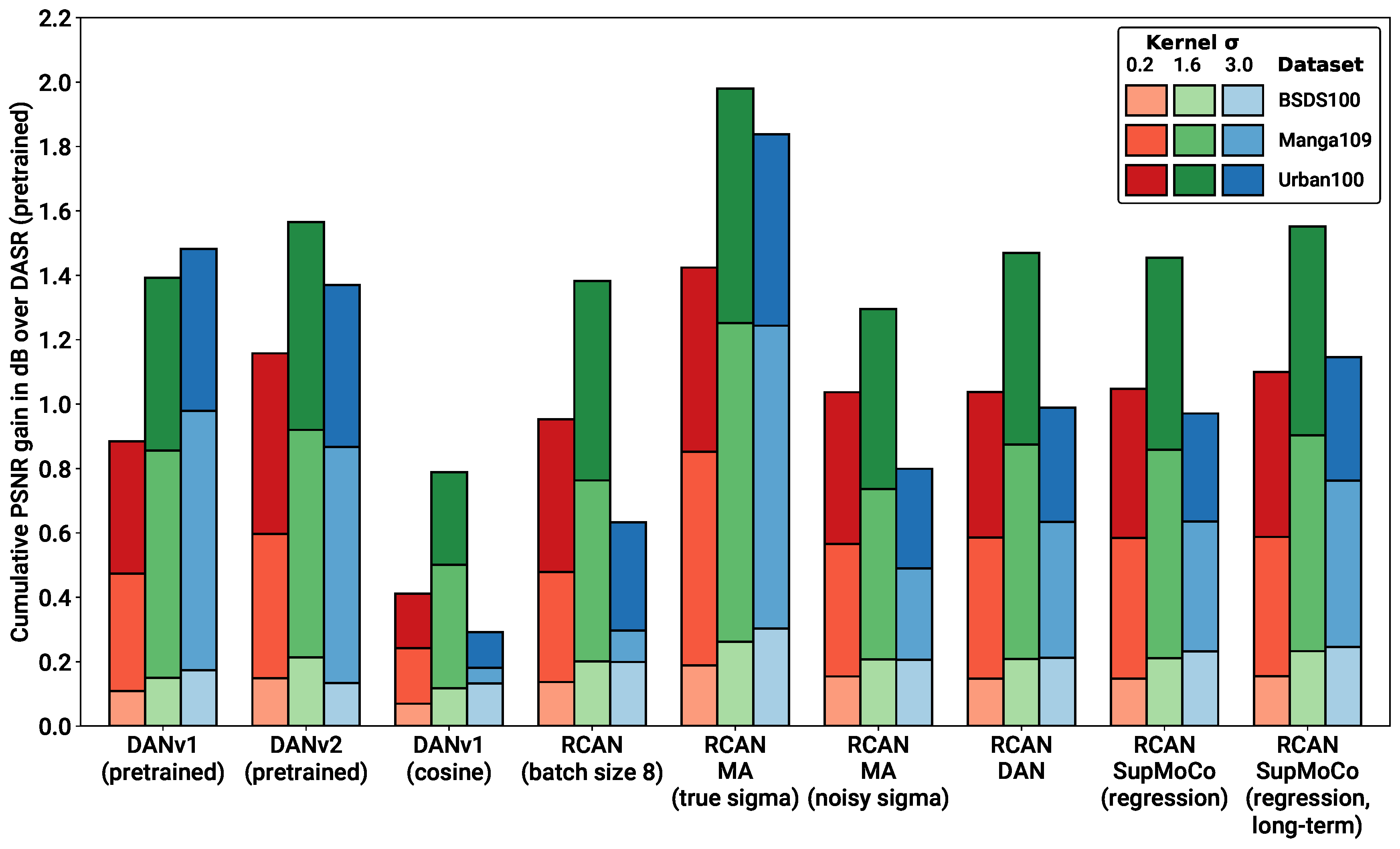
- Non-blind models: The non-blind models fed with the true blur kernel width achieve the best performance of all the models studied. This is true both for RCAN and HAN, with HAN having a slight edge overall. The wide margin over all other blind models clearly shows that significantly improved performance is possible if the degradation prediction system can be improved. We also trained and tested a model (RCAN-MA (noisy sigma)) which was provided with the normalised values corrupted by noise (mean 0, standard deviation 0.1). This error level is slightly higher than that of the DAN models tested ( Figure 7A), allowing this model to act as a performance reference for our estimation methods.
- RCAN-DAN models: As observed in Figure 7, the DAN models that were trained from scratch are significantly worse than the RCAN models, including the fully non-blind RCAN, across all datasets and values, as shown in Figure 8 and Figure 9 respectively. The RCAN-DAN models show a consistent performance boost over RCAN across the board. As noted earlier in Section 4.2, predicting PCA-reduced kernels appears to provide no advantage over directly predicting the kernel width.
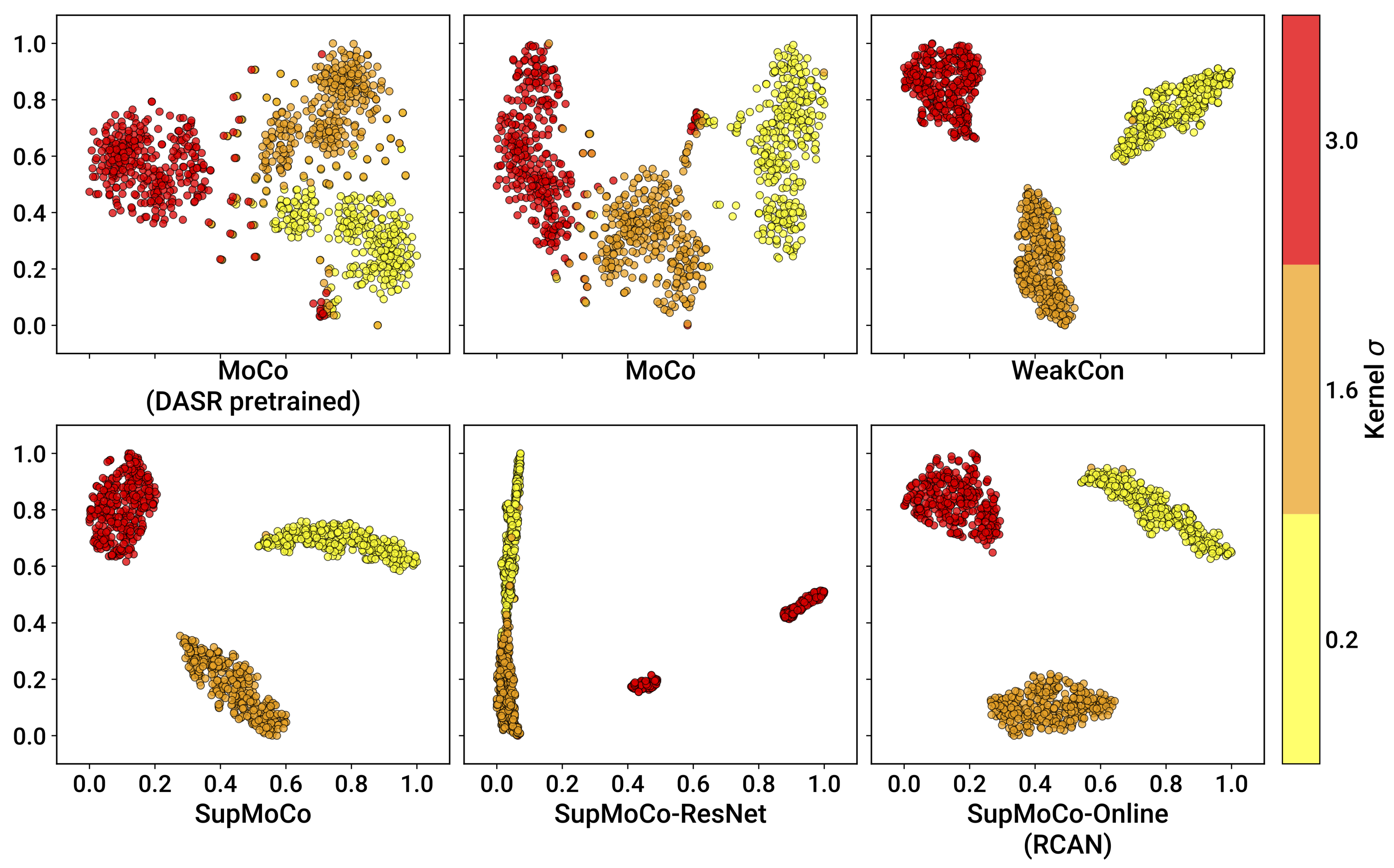
- RCAN-Contrastive models: For the contrastive models, the results are much less clear-cut. The different contrastive blind models exhibit superior performance to RCAN under most conditions (except for Urban100), but none of the algorithms tested (MoCo, SupMoCo, WeakCon and direct regression) seem to provide any particular advantage over each other. The encoder trained with combined regression and SupMoCo appears to provide a slight boost over the other techniques (Figure 8), but this is not consistent across the datasets and values analysed. This is a surprising result, given that the clear clusters formed by SupMoCo and WeakCon (as shown in Figure 6) would have been expected to improve the encoders’ predictive power. We hypothesise that the encoded representation is difficult for even deep learning models to interpret, and a clear-cut route from the encoded vector to the actual blur may be difficult to produce. We also observe that both the RCAN-DAN and RCAN-SupMoCo models clearly surpass the noisy sigma non-blind RCAN model on datasets with medium and high , while they perform slightly worse on datasets with low . This matches the results in Figure 7, where it is clear that the performance of all predictors suffer when is low.
- HAN models: Upgraded HAN models appear to follow similar trends as RCAN models. The inclusion of DAN provides a clear boost in performance, but this time the inclusion of the SupMoCo-regression predictor seems to only boost performance when is high.
- Extensions: We also trained a RCAN-DAN model where we pre-initialised the predictor with that from the pretrained DANv1 model. The minor improvements indicate that, for the most part, the predictor is achieving similar prediction accuracy to that of the pretrained models (as is also indicated in Figure 7). We also extended the training of the baseline RCAN and the RCAN-SupMoCo-regression model to 2200 epochs. The expanded training continues to improve performance and, perhaps crucially, the contrastive model continues to show a margin of improvement over the baseline RCAN model. In fact, this extended model starts to achieve similar or better performance than the pretrained DAN models (shown both in Table 3 and Figure 9). This is achieved with a significantly shorter training time (2200 vs. epochs) and a fixed set of degradations, indicating that our models would surpass the performance of the pretrained DAN models if trained with the same conditions.
4.5. Complex Degradation Prediction
4.5.1. Contrastive Learning
- We first pre-trained the encoder with an online pipeline of noise (same parameters as the full complex pipeline, but with an equal probability to select grey or colour noise) and bicubic downsampling. We found that this pre-training helps reduce loss stagnation for the SupMoCo encoder, so we applied this to all encoders. The SupMoCo encoder was trained with double precision at this stage. We used 3 positive patches for SupMoCo and 1 positive patch for both MoCo and WeakCon.
- After 1099 epochs, we started training the encoder on the full online complex pipeline (Section 4.1). The SupMoCo encoder was switched to triple precision from this point onwards.
- We stopped all encoders after 2001 total epochs, and evaluated them at this checkpoint.
- For SupMoCo, the decision tree in Section 3.5.2 was used to assign class labels. For WeakCon, was computed as the Euclidean distance between query/negative sample vectors containing: the vertical and horizontal blur , the Gaussian/Poisson sigma/scale, respectively, and the JPEG/JM H.264 quality factor/QPI, respectively, (6 elements total). All values were normalised to prior to computation.
4.5.2. Iterative Parameter Regression
- Individual elements for the following blur parameters: vertical and horizontal , rotation, individual for generalised Gaussian and plateau kernels and the sinc cutoff frequency. Whenever one of these elements was unused (e.g., cutoff frequency for Gaussian kernels), this was set to 0. All elements were normalised to according to their respective ranges (Section 4.1).
- Four boolean (0 or 1) elements categorising whether the kernel shape was:
- Isotropic or anisotropic
- −
- Generalised
- −
- Plateau-type
- −
- Sinc
- Individual elements for the Gaussian sigma and Poisson scale (both normalised to ).
- A boolean indicating whether the noise was colour or grey type.
- Individual elements for the JM H.264 QPI and JPEG quality factor (both normalised to ).
4.6. Blind SR on Complex Pipeline
- Compression- and noise-only scenarios: In these scenarios, the RCAN-DAN model shows clear improvement over all other baseline and contrastive encoders (apart from some cases on Manga109). Improvement is most significant in the compression scenarios.
- Multiple combinations: In the multiple degradation scenarios, the DAN model consistently overtakes the baselines, but PSNR/SSIM increases are minimal.
4.7. Blind SR on Real LR Images
4.8. Results Summary
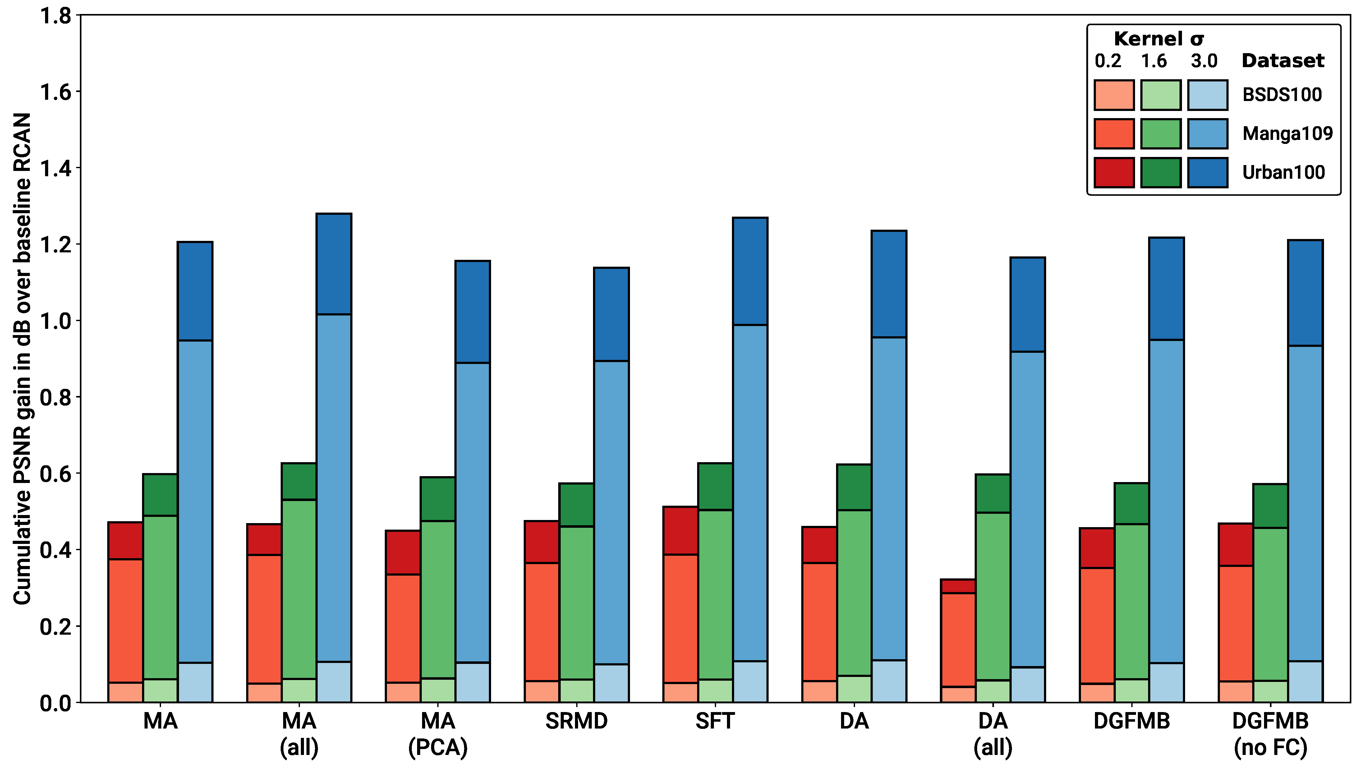
- In Section 4.2, we show that all of the metadata insertion mechanisms tested provide roughly the same SR performance boost when feeding a large network such as RCAN with non-blind blurring metadata. Furthermore, adding repeated blocks through the network provides little to no benefit. Given this result, we propose MA as our metadata insertion block of choice, as it provides identical SR performance as the other options considered, with very low complexity. Other metadata blocks could prove optimal in other scenarios (such as other degradations or with other networks), which would require further systematic investigation to determine.
- Section 4.3 provides a comparison of the prediction performance of the different algorithms considered on the simple blur pipeline. The contrastive algorithms clearly cluster images by the applied blur kernel width, with the semi-supervised algorithms providing the most well-defined separation between different values. The regression and iterative mechanisms are capable of explicitly predicting the blur kernel width with high accuracy, except at the lower extreme. Our prediction mechanisms combined with RCAN match the performance of the pretrained DAN models with significantly less training time.
- Section 4.4 compares the testing results of blind models built with our framework with baseline models from the literature. Each prediction mechanism considered elevates RCAN’s SR performance above its baseline value, for both PSNR and SSIM. In particular, the iterative mechanism provided the largest performance boost. For more complex models such as HAN and Real-ESRGAN, contrastive methods provide less benefit, but the iterative mechanism still shows clear improvements. Our models significantly overtake the SOTA blind DAN network when trained for the same length of time. In addition, our models approach or surpass the performance of the pretrained DANv1 and DANv2 checkpoints provided by their authors, which were trained for a significantly longer period of time.
- In Section 4.5 and Section 4.6, we modify our prediction mechanisms to deal with a more complex pipeline of blurring, noise and compression, and attach these to the RCAN network. We show that the contrastive predictors can reliably cluster compression and noise, but blur kernel clustering is significantly weaker. Similarly, the iterative predictors are highly accurate when predicting compression/noise parameters, but are much less reliable for blur parameters.When testing their SR performance, the contrastive encoders seem to provide little to no benefit to RCAN’s performance. On the other hand, the DAN models reliably improve the baseline performance across various scenarios, albeit with limited improvements when all degradations are present at once. We anticipate that performance can be significantly improved with further advances to the prediction mechanisms and consider our results as a baseline for further exploration.
- Section 4.7 showcases the results of our models when applied to real-world LR images. Our complex pipeline models produce significantly better results than the pretrained DAN models and are capable of reversing noise, compression and blurring in various scenarios.
5. Conclusions
Supplementary Materials
Author Contributions
Funding
Institutional Review Board Statement
Informed Consent Statement
Data Availability Statement
Conflicts of Interest
References
- Gupta, R.; Sharma, A.; Kumar, A. Super-Resolution using GANs for Medical Imaging. Procedia Comput. Sci. 2020, 173, 28–35. [Google Scholar] [CrossRef]
- Ahmad, W.; Ali, H.; Shah, Z.; Azmat, S. A new generative adversarial network for medical images super resolution. Sci. Rep. 2022, 12, 9533. [Google Scholar] [CrossRef] [PubMed]
- Haut, J.M.; Fernandez-Beltran, R.; Paoletti, M.E.; Plaza, J.; Plaza, A.; Pla, F. A New Deep Generative Network for Unsupervised Remote Sensing Single-Image Super-Resolution. IEEE Trans. Geosci. Remote Sens. 2018, 56, 6792–6810. [Google Scholar] [CrossRef]
- Wang, P.; Bayram, B.; Sertel, E. A comprehensive review on deep learning based remote sensing image super-resolution methods. Earth-Sci. Rev. 2022, 232, 104110. [Google Scholar] [CrossRef]
- Zhang, J.; Xu, T.; Li, J.; Jiang, S.; Zhang, Y. Single-Image Super Resolution of Remote Sensing Images with Real-World Degradation Modeling. Remote Sens. 2022, 14, 2895. [Google Scholar] [CrossRef]
- Chen, H.; He, X.; Qing, L.; Wu, Y.; Ren, C.; Sheriff, R.E.; Zhu, C. Real-world single image super-resolution: A brief review. Inf. Fusion 2022, 79, 124–145. [Google Scholar] [CrossRef]
- Rasti, P.; Uiboupin, T.; Escalera, S.; Anbarjafari, G. Convolutional Neural Network Super Resolution for Face Recognition in Surveillance Monitoring. In Proceedings of the Articulated Motion and Deformable Objects, Palma de Mallorca, Spain, 13–15 July 2016; Perales, F.J., Kittler, J., Eds.; Springer International Publishing: Cham, Switzerland, 2016; pp. 175–184. [Google Scholar] [CrossRef]
- Zhang, Y.; Li, K.; Li, K.; Wang, L.; Zhong, B.; Fu, Y. Image Super-Resolution Using Very Deep Residual Channel Attention Networks. In Proceedings of the Computer Vision—ECCV 2018, Munich, Germany, 8–14 September 2018; Ferrari, V., Hebert, M., Sminchisescu, C., Weiss, Y., Eds.; Springer International Publishing: Cham, Switzerland, 2018; pp. 294–310. [Google Scholar] [CrossRef]
- Dai, T.; Cai, J.; Zhang, Y.; Xia, S.T.; Zhang, L. Second-Order Attention Network for Single Image Super-Resolution. In Proceedings of the 2019 IEEE/CVF Conference on Computer Vision and Pattern Recognition (CVPR), Long Beach, CA, USA, 15–20 June 2019; pp. 11057–11066. [Google Scholar] [CrossRef]
- Niu, B.; Wen, W.; Ren, W.; Zhang, X.; Yang, L.; Wang, S.; Zhang, K.; Cao, X.; Shen, H. Single Image Super-Resolution via a Holistic Attention Network. In Proceedings of the Computer Vision—ECCV 2020, Glasgow, UK, 23–28 August 2020; Vedaldi, A., Bischof, H., Brox, T., Frahm, J.M., Eds.; Springer International Publishing: Cham, Switzerland, 2020; pp. 191–207. [Google Scholar] [CrossRef]
- Vella, M.; Mota, J.F.C. Robust Single-Image Super-Resolution via CNNs and TV-TV Minimization. IEEE Trans. Image Process. 2021, 30, 7830–7841. [Google Scholar] [CrossRef]
- Liang, J.; Cao, J.; Sun, G.; Zhang, K.; Van Gool, L.; Timofte, R. SwinIR: Image Restoration Using Swin Transformer. In Proceedings of the 2021 IEEE/CVF International Conference on Computer Vision Workshops (ICCVW), Montreal, QC, Canada, 11–17 October 2021; pp. 1833–1844. [Google Scholar] [CrossRef]
- Zhang, X.; Zeng, H.; Guo, S.; Zhang, L. Efficient Long-Range Attention Network for Image Super-Resolution. In Proceedings of the Computer Vision—ECCV 2022, Tel Aviv, Israel, 23–27 October 2022; Avidan, S., Brostow, G., Cissé, M., Farinella, G.M., Hassner, T., Eds.; Springer Nature Switzerland: Cham, Switzerland, 2022; pp. 649–667. [Google Scholar] [CrossRef]
- Ledig, C.; Theis, L.; Huszár, F.; Caballero, J.; Cunningham, A.; Acosta, A.; Aitken, A.; Tejani, A.; Totz, J.; Wang, Z.; et al. Photo-Realistic Single Image Super-Resolution Using a Generative Adversarial Network. In Proceedings of the 2017 IEEE Conference on Computer Vision and Pattern Recognition (CVPR), Honolulu, HI, USA, 21–26 July 2017; pp. 105–114. [Google Scholar] [CrossRef]
- Wang, X.; Yu, K.; Wu, S.; Gu, J.; Liu, Y.; Dong, C.; Qiao, Y.; Loy, C.C. ESRGAN: Enhanced Super-Resolution Generative Adversarial Networks. In Proceedings of the Computer Vision—ECCV 2018 Workshops, Munich, Germany, 8–14 September 2018; Leal-Taixé, L., Roth, S., Eds.; Springer International Publishing: Cham, Switzerland, 2019; pp. 63–79. [Google Scholar] [CrossRef]
- Wang, X.; Xie, L.; Dong, C.; Shan, Y. Real-ESRGAN: Training Real-World Blind Super-Resolution with Pure Synthetic Data. In Proceedings of the 2021 IEEE/CVF International Conference on Computer Vision Workshops (ICCVW), Montreal, QC, Canada, 11–17 October 2021; pp. 1905–1914. [Google Scholar] [CrossRef]
- Zhang, W.; Shi, G.; Liu, Y.; Dong, C.; Wu, X.M. A Closer Look at Blind Super-Resolution: Degradation Models, Baselines, and Performance Upper Bounds. In Proceedings of the 2022 IEEE/CVF Conference on Computer Vision and Pattern Recognition Workshops (CVPRW), New Orleans, LA, USA, 19–20 June 2022; pp. 527–536. [Google Scholar] [CrossRef]
- Liu, A.; Liu, Y.; Gu, J.; Qiao, Y.; Dong, C. Blind Image Super-Resolution: A Survey and Beyond. IEEE Trans. Pattern Anal. Mach. Intell. 2022, 1–19. [Google Scholar] [CrossRef]
- Zhang, K.; Liang, J.; Van Gool, L.; Timofte, R. Designing a Practical Degradation Model for Deep Blind Image Super-Resolution. In Proceedings of the 2021 IEEE/CVF International Conference on Computer Vision (ICCV), Montreal, QC, Canada, 10–17 October 2021; pp. 4791–4800. [Google Scholar] [CrossRef]
- Jiang, J.; Wang, C.; Liu, X.; Ma, J. Deep Learning-Based Face Super-Resolution: A Survey. ACM Comput. Surv. 2021, 55, 1–36. [Google Scholar] [CrossRef]
- Köhler, T.; Bätz, M.; Naderi, F.; Kaup, A.; Maier, A.; Riess, C. Toward Bridging the Simulated-to-Real Gap: Benchmarking Super-Resolution on Real Data. IEEE Trans. Pattern Anal. Mach. Intell. 2020, 42, 2944–2959. [Google Scholar] [CrossRef]
- Gu, J.; Lu, H.; Zuo, W.; Dong, C. Blind Super-Resolution With Iterative Kernel Correction. In Proceedings of the 2019 IEEE/CVF Conference on Computer Vision and Pattern Recognition (CVPR), Long Beach, CA, USA, 15–20 June 2019; pp. 1604–1613. [Google Scholar] [CrossRef]
- Luo, Z.; Huang, Y.; Li, S.; Wang, L.; Tan, T. Unfolding the Alternating Optimization for Blind Super Resolution. In Proceedings of the Advances in Neural Information Processing Systems 33, Virtual, 6–12 December 2020; Larochelle, H., Ranzato, M., Hadsell, R., Balcan, M., Lin, H., Eds.; Curran Associates, Inc.: Red Hook, NY, USA, 2020; Volume 33, pp. 5632–5643. [Google Scholar]
- Wang, L.; Wang, Y.; Dong, X.; Xu, Q.; Yang, J.; An, W.; Guo, Y. Unsupervised Degradation Representation Learning for Blind Super-Resolution. In Proceedings of the 2021 IEEE/CVF Conference on Computer Vision and Pattern Recognition (CVPR), Nashville, TN, USA, 20–25 June 2021; pp. 10576–10585. [Google Scholar] [CrossRef]
- Zhang, Y.; Dong, L.; Yang, H.; Qing, L.; He, X.; Chen, H. Weakly-supervised contrastive learning-based implicit degradation modeling for blind image super-resolution. Knowl.-Based Syst. 2022, 249, 108984. [Google Scholar] [CrossRef]
- Aquilina, M.; Galea, C.; Abela, J.; Camilleri, K.P.; Farrugia, R.A. Improving Super-Resolution Performance Using Meta-Attention Layers. IEEE Signal Process. Lett. 2021, 28, 2082–2086. [Google Scholar] [CrossRef]
- Luo, Z.; Huang, H.; Yu, L.; Li, Y.; Fan, H.; Liu, S. Deep Constrained Least Squares for Blind Image Super-Resolution. In Proceedings of the 2022 IEEE/CVF Conference on Computer Vision and Pattern Recognition (CVPR), New Orleans, LA, USA, 18–24 June 2022; pp. 17642–17652. [Google Scholar] [CrossRef]
- Dong, C.; Loy, C.C.; He, K.; Tang, X. Learning a Deep Convolutional Network for Image Super-Resolution. In Proceedings of the Computer Vision—ECCV 2014, Zurich, Switzerland, 6–12 September 2014; Fleet, D., Pajdla, T., Schiele, B., Tuytelaars, T., Eds.; Springer International Publishing: Cham, Switzerland, 2014; pp. 184–199. [Google Scholar] [CrossRef]
- Bulat, A.; Tzimiropoulos, G. Super-FAN: Integrated Facial Landmark Localization and Super-Resolution of Real-World Low Resolution Faces in Arbitrary Poses with GANs. In Proceedings of the 2018 IEEE/CVF Conference on Computer Vision and Pattern Recognition (CVPR), Salt Lake City, UT, USA, 18–23 June 2018; pp. 109–117. [Google Scholar] [CrossRef]
- Huang, H.; He, R.; Sun, Z.; Tan, T. Wavelet Domain Generative Adversarial Network for Multi-scale Face Hallucination. Int. J. Comput. Vis. 2019, 127, 763–784. [Google Scholar] [CrossRef]
- Yu, X.; Fernando, B.; Ghanem, B.; Porikli, F.; Hartley, R. Face Super-Resolution Guided by Facial Component Heatmaps. In Proceedings of the Computer Vision—ECCV 2018, Munich, Germany, 8–14 September 2018; Ferrari, V., Hebert, M., Sminchisescu, C., Weiss, Y., Eds.; Springer International Publishing: Cham, Swizerland, 2018; pp. 219–235. [Google Scholar] [CrossRef]
- Chen, Y.; Tai, Y.; Liu, X.; Shen, C.; Yang, J. FSRNet: End-to-End Learning Face Super-Resolution with Facial Priors. In Proceedings of the 2018 IEEE/CVF Conference on Computer Vision and Pattern Recognition (CVPR), Salt Lake City, UT, USA, 18–23 June 2018; pp. 2492–2501. [Google Scholar] [CrossRef]
- Huang, H.; He, R.; Sun, Z.; Tan, T. Wavelet-SRNet: A Wavelet-Based CNN for Multi-scale Face Super Resolution. In Proceedings of the 2017 IEEE International Conference on Computer Vision (ICCV), Venice, Italy, 22–29 October 2017; pp. 1698–1706. [Google Scholar] [CrossRef]
- Lu, Z.; Jiang, X.; Kot, A. Deep Coupled ResNet for Low-Resolution Face Recognition. IEEE Signal Process. Lett. 2018, 25, 526–530. [Google Scholar] [CrossRef]
- Cao, Q.; Lin, L.; Shi, Y.; Liang, X.; Li, G. Attention-Aware Face Hallucination via Deep Reinforcement Learning. In Proceedings of the 2017 IEEE Conference on Computer Vision and Pattern Recognition (CVPR), Honolulu, HI, USA, 21–26 July 2017; pp. 1656–1664. [Google Scholar] [CrossRef]
- Yu, X.; Fernando, B.; Hartley, R.; Porikli, F. Super-Resolving Very Low-Resolution Face Images with Supplementary Attributes. In Proceedings of the 2018 IEEE/CVF Conference on Computer Vision and Pattern Recognition (CVPR), Salt Lake City, UT, USA, 18–23 June 2018; pp. 908–917. [Google Scholar] [CrossRef]
- Nguyen, N.L.; Anger, J.; Davy, A.; Arias, P.; Facciolo, G. Self-Supervised Super-Resolution for Multi-Exposure Push-Frame Satellites. In Proceedings of the 2022 IEEE/CVF Conference on Computer Vision and Pattern Recognition (CVPR), New Orleans, LA, USA, 18–24 June 2022; pp. 1848–1858. [Google Scholar] [CrossRef]
- Luo, Z.; Huang, Y.; Li, S.; Wang, L.; Tan, T. End-to-end Alternating Optimization for Blind Super Resolution. arXiv 2021. [Google Scholar] [CrossRef]
- Zhang, K.; Zuo, W.; Zhang, L. Learning a Single Convolutional Super-Resolution Network for Multiple Degradations. In Proceedings of the 2018 IEEE/CVF Conference on Computer Vision and Pattern Recognition (CVPR), Salt Lake City, UT, USA, 18–23 June 2018; pp. 3262–3271. [Google Scholar] [CrossRef]
- Xiao, J.; Yong, H.; Zhang, L. Degradation Model Learning for Real-World Single Image Super-Resolution. In Proceedings of the Computer Vision—ACCV 2020, Kyoto, Japan, 30 November–4 December 2020; Ishikawa, H., Liu, C.L., Pajdla, T., Shi, J., Eds.; Springer International Publishing: Cham, Swizerland, 2021; pp. 84–101. [Google Scholar] [CrossRef]
- Yue, Z.; Zhao, Q.; Xie, J.; Zhang, L.; Meng, D.; Wong, K.Y.K. Blind Image Super-Resolution With Elaborate Degradation Modeling on Noise and Kernel. In Proceedings of the 2022 IEEE/CVF Conference on Computer Vision and Pattern Recognition (CVPR), New Orleans, LA, USA, 18–24 June 2022; pp. 2128–2138. [Google Scholar] [CrossRef]
- Emad, M.; Peemen, M.; Corporaal, H. MoESR: Blind Super-Resolution using Kernel-Aware Mixture of Experts. In Proceedings of the 2022 IEEE/CVF Winter Conference on Applications of Computer Vision (WACV), Waikoloa, HI, USA, 3–8 January 2022; pp. 4009–4018. [Google Scholar] [CrossRef]
- Kang, X.; Li, J.; Duan, P.; Ma, F.; Li, S. Multilayer Degradation Representation-Guided Blind Super-Resolution for Remote Sensing Images. IEEE Trans. Geosci. Remote Sens. 2022, 60, 1–12. [Google Scholar] [CrossRef]
- Liu, P.; Zhang, H.; Cao, Y.; Liu, S.; Ren, D.; Zuo, W. Learning cascaded convolutional networks for blind single image super-resolution. Neurocomputing 2020, 417, 371–383. [Google Scholar] [CrossRef]
- He, K.; Zhang, X.; Ren, S.; Sun, J. Deep Residual Learning for Image Recognition. In Proceedings of the 2016 IEEE Conference on Computer Vision and Pattern Recognition (CVPR), Las Vegas, NV, USA, 27–30 June 2016; pp. 770–778. [Google Scholar] [CrossRef]
- Lim, B.; Son, S.; Kim, H.; Nah, S.; Mu Lee, K. Enhanced Deep Residual Networks for Single Image Super-Resolution. In Proceedings of the 2017 IEEE Conference on Computer Vision and Pattern Recognition Workshops (CVPRW), Honolulu, HI, USA, 21–26 July 2017; pp. 1132–1140. [Google Scholar] [CrossRef]
- Li, W.; Lu, X.; Qian, S.; Lu, J.; Zhang, X.; Jia, J. On Efficient Transformer and Image Pre-training for Low-level Vision. arXiv 2021. [Google Scholar] [CrossRef]
- Lu, Z.; Li, J.; Liu, H.; Huang, C.; Zhang, L.; Zeng, T. Transformer for Single Image Super-Resolution. In Proceedings of the 2022 IEEE/CVF Conference on Computer Vision and Pattern Recognition Workshops (CVPRW), New Orleans, LA, USA, 19–20 June 2022; pp. 456–465. [Google Scholar] [CrossRef]
- Liu, Z.; Lin, Y.; Cao, Y.; Hu, H.; Wei, Y.; Zhang, Z.; Lin, S.; Guo, B. Swin Transformer: Hierarchical Vision Transformer using Shifted Windows. In Proceedings of the 2021 IEEE/CVF International Conference on Computer Vision (ICCV), Montreal, QC, Canada, 10–17 October 2021; pp. 9992–10002. [Google Scholar] [CrossRef]
- Chen, X.; Wang, X.; Zhou, J.; Dong, C. Activating More Pixels in Image Super-Resolution Transformer. arXiv 2022. [Google Scholar] [CrossRef]
- Ha, V.K.; Ren, J.C.; Xu, X.Y.; Zhao, S.; Xie, G.; Masero, V.; Hussain, A. Deep Learning Based Single Image Super-Resolution: A Survey. Int. J. Autom. Comput. 2019, 16, 413–426. [Google Scholar] [CrossRef]
- Wang, Z.; Chen, J.; Hoi, S.C.H. Deep Learning for Image Super-Resolution: A Survey. IEEE Trans. Pattern Anal. Mach. Intell. 2021, 43, 3365–3387. [Google Scholar] [CrossRef] [PubMed]
- Xu, Y.S.; Tseng, S.Y.R.; Tseng, Y.; Kuo, H.K.; Tsai, Y.M. Unified Dynamic Convolutional Network for Super-Resolution With Variational Degradations. In Proceedings of the 2020 IEEE/CVF Conference on Computer Vision and Pattern Recognition (CVPR), Seattle, WA, USA, 13–19 June 2020; pp. 12493–12502. [Google Scholar] [CrossRef]
- Cornillère, V.; Djelouah, A.; Yifan, W.; Sorkine-Hornung, O.; Schroers, C. Blind Image Super-Resolution with Spatially Variant Degradations. ACM Trans. Graph. 2019, 38. [Google Scholar] [CrossRef]
- Yin, G.; Wang, W.; Yuan, Z.; Ji, W.; Yu, D.; Sun, S.; Chua, T.S.; Wang, C. Conditional Hyper-Network for Blind Super-Resolution With Multiple Degradations. IEEE Trans. Image Process. 2022, 31, 3949–3960. [Google Scholar] [CrossRef]
- Kim, S.Y.; Sim, H.; Kim, M. KOALAnet: Blind Super-Resolution using Kernel-Oriented Adaptive Local Adjustment. In Proceedings of the 2021 IEEE/CVF Conference on Computer Vision and Pattern Recognition (CVPR), Nashville, TN, USA, 20–25 June 2021; pp. 10606–10615. [Google Scholar] [CrossRef]
- Bell-Kligler, S.; Shocher, A.; Irani, M. Blind Super-Resolution Kernel Estimation Using an Internal-GAN. In Proceedings of the Advances in Neural Information Processing Systems 32, Vancouver, BC, Canada, 8–14 December 2019; Wallach, H., Larochelle, H., Beygelzimer, A., d’Alché-Buc, F., Fox, E., Garnett, R., Eds.; Curran Associates, Inc.: Red Hook, NY, USA, 2019; Volume 32, pp. 284–293. [Google Scholar]
- Shocher, A.; Cohen, N.; Irani, M. Zero-Shot Super-Resolution Using Deep Internal Learning. In Proceedings of the 2018 IEEE/CVF Conference on Computer Vision and Pattern Recognition (CVPR), Salt Lake City, UT, USA, 18–23 June 2018; pp. 3118–3126. [Google Scholar] [CrossRef]
- Yuan, Y.; Liu, S.; Zhang, J.; Zhang, Y.; Dong, C.; Lin, L. Unsupervised Image Super-Resolution Using Cycle-in-Cycle Generative Adversarial Networks. In Proceedings of the 2018 IEEE/CVF Conference on Computer Vision and Pattern Recognition Workshops (CVPRW), Salt Lake City, UT, USA, 18–22 June 2018; pp. 814–823. [Google Scholar] [CrossRef]
- Zhou, Y.; Deng, W.; Tong, T.; Gao, Q. Guided Frequency Separation Network for Real-World Super-Resolution. In Proceedings of the 2020 IEEE/CVF Conference on Computer Vision and Pattern Recognition Workshops (CVPRW), Seattle, WA, USA, 14–19 June 2020; pp. 1722–1731. [Google Scholar] [CrossRef]
- Maeda, S. Unpaired Image Super-Resolution Using Pseudo-Supervision. In Proceedings of the 2020 IEEE/CVF Conference on Computer Vision and Pattern Recognition (CVPR), Seattle, WA, USA, 13–19 June 2020; pp. 288–297. [Google Scholar] [CrossRef]
- Bulat, A.; Yang, J.; Tzimiropoulos, G. To Learn Image Super-Resolution, Use a GAN to Learn How to Do Image Degradation First. In Proceedings of the Computer Vision—ECCV 2018, Munich, Germany, 8–14 September 2018; Ferrari, V., Hebert, M., Sminchisescu, C., Weiss, Y., Eds.; Springer International Publishing: Cham, Switzerland, 2018; pp. 187–202. [Google Scholar] [CrossRef]
- Fritsche, M.; Gu, S.; Timofte, R. Frequency Separation for Real-World Super-Resolution. In Proceedings of the 2019 IEEE/CVF International Conference on Computer Vision Workshop (ICCVW), Seoul, South Korea, 27–28 October 2019; pp. 3599–3608. [Google Scholar] [CrossRef]
- Majumder, O.; Ravichandran, A.; Maji, S.; Achille, A.; Polito, M.; Soatto, S. Supervised Momentum Contrastive Learning for Few-Shot Classification. arXiv 2021. [Google Scholar] [CrossRef]
- Doersch, C.; Gupta, A.; Zisserman, A. CrossTransformers: Spatially-aware few-shot transfer. In Proceedings of the Advances in Neural Information Processing Systems 33, Virtual, 6–12 December 2020; Larochelle, H., Ranzato, M., Hadsell, R., Balcan, M., Lin, H., Eds.; Curran Associates, Inc.: Red Hook, NY, USA, 2020; Volume 33, pp. 21981–21993. [Google Scholar]
- Khosla, P.; Teterwak, P.; Wang, C.; Sarna, A.; Tian, Y.; Isola, P.; Maschinot, A.; Liu, C.; Krishnan, D. Supervised Contrastive Learning. In Proceedings of the Advances in Neural Information Processing Systems 33, Virtual, 6–12 December 2020; Larochelle, H., Ranzato, M., Hadsell, R., Balcan, M., Lin, H., Eds.; Curran Associates, Inc.: Red Hook, NY, USA, 2020; Volume 33, pp. 18661–18673. [Google Scholar]
- Zhang, Z.; Sabuncu, M.R. Generalized Cross Entropy Loss for Training Deep Neural Networks with Noisy Labels. In Proceedings of the Advances in Neural Information Processing Systems 31, Montreal, QC, Canada, 2–8 December 2018; Bengio, S., Wallach, H., Larochelle, H., Grauman, K., Cesa-Bianchi, N., Garnett, R., Eds.; Curran Associates, Inc.: Red Hook, NY, USA, 2018; Volume 31, pp. 8792–8802. [Google Scholar]
- Sukhbaatar, S.; Bruna, J.; Paluri, M.; Bourdev, L.; Fergus, R. Training Convolutional Networks with Noisy Labels. arXiv 2014. [Google Scholar] [CrossRef]
- Elsayed, G.; Krishnan, D.; Mobahi, H.; Regan, K.; Bengio, S. Large Margin Deep Networks for Classification. In Proceedings of the Advances in Neural Information Processing Systems 31, Montreal, QC, Canada, 2–8 December 2018; Bengio, S., Wallach, H., Larochelle, H., Grauman, K., Cesa-Bianchi, N., Garnett, R., Eds.; Curran Associates, Inc.: Red Hook, NY, USA, 2018; Volume 31, pp. 850–860. [Google Scholar]
- Cao, K.; Wei, C.; Gaidon, A.; Arechiga, N.; Ma, T. Learning Imbalanced Datasets with Label-Distribution-Aware Margin Loss. In Proceedings of the Advances in Neural Information Processing Systems 32, Vancouver, BC, Canada, 8–14 December 2019; Wallach, H., Larochelle, H., Beygelzimer, A., d’Alché-Buc, F., Fox, E., Garnett, R., Eds.; Curran Associates, Inc.: Red Hook, NY, USA, 2019; Volume 32, pp. 1567–1578. [Google Scholar]
- Liu, W.; Wen, Y.; Yu, Z.; Yang, M. Large-Margin Softmax Loss for Convolutional Neural Networks. In Proceedings of the 33rd International Conference on Machine Learning (ICML), New York, NY, USA, 20–22 June 2019; Balcan, M.F., Weinberger, Eds.; PMLR: Cambridge, MA, USA, 2016; Volume 48, pp. 507–516. [Google Scholar]
- Chen, T.; Kornblith, S.; Norouzi, M.; Hinton, G. A Simple Framework for Contrastive Learning of Visual Representations. In Proceedings of the 37th International Conference on Machine Learning (ICML), Virtual, 13–18 July 2020; PMLR: Cambridge, MA, USA, 2020; Volume 119, pp. 1597–1607. [Google Scholar]
- He, K.; Fan, H.; Wu, Y.; Xie, S.; Girshick, R. Momentum Contrast for Unsupervised Visual Representation Learning. In Proceedings of the 2020 IEEE/CVF Conference on Computer Vision and Pattern Recognition (CVPR), Seattle, WA, USA, 13–19 June 2020; pp. 9726–9735. [Google Scholar] [CrossRef]
- Chen, X.; Fan, H.; Girshick, R.; He, K. Improved Baselines with Momentum Contrastive Learning. arXiv 2020. [Google Scholar] [CrossRef]
- Oord, A.v.d.; Li, Y.; Vinyals, O. Representation Learning with Contrastive Predictive Coding. arXiv 2018. [Google Scholar] [CrossRef]
- Sühring, K.; Tourapis, A.M.; Leontaris, A.; Sullivan, G. H.264/14496-10 AVC Reference Software Manual (revised for JM 19.0). 2015. Available online: http://iphome.hhi.de/suehring/tml/ (accessed on 2 July 2021).
- Agustsson, E.; Timofte, R. NTIRE 2017 Challenge on Single Image Super-Resolution: Dataset and Study. In Proceedings of the 2017 IEEE Conference on Computer Vision and Pattern Recognition Workshops (CVPRW), Honolulu, HI, USA, 21–26 July 2017; pp. 1122–1131. [Google Scholar] [CrossRef]
- Timofte, R.; Agustsson, E.; Van Gool, L.; Yang, M.H.; Zhang, L. NTIRE 2017 Challenge on Single Image Super-Resolution: Methods and Results. In Proceedings of the 2017 IEEE Conference on Computer Vision and Pattern Recognition Workshops (CVPRW), Honolulu, HI, USA, 21–26 July 2017; pp. 1110–1121. [Google Scholar] [CrossRef]
- Bevilacqua, M.; Roumy, A.; Guillemot, C.; Morel, M.l.A. Low-Complexity Single-Image Super-Resolution Based on Nonnegative Neighbor Embedding. In Proceedings of the British Machine Vision Conference, Surrey, UK, 3–7 September 2012; Bowden, R., Collomosse, J., Mikolajczyk, K., Eds.; BMVA Press: Durham, UK, 2012; pp. 135.1–135.10. [Google Scholar] [CrossRef]
- Zeyde, R.; Elad, M.; Protter, M. On Single Image Scale-Up Using Sparse-Representations. In Proceedings of the Curves and Surfaces, Avignon, France, 24–30 June 2010; Boissonnat, J.D., Chenin, P., Cohen, A., Gout, C., Lyche, T., Mazure, M.L., Schumaker, L., Eds.; Springer: Berlin/Heidelberg, Germany, 2012; pp. 711–730. [Google Scholar] [CrossRef]
- Arbeláez, P.; Maire, M.; Fowlkes, C.; Malik, J. Contour Detection and Hierarchical Image Segmentation. IEEE Trans. Pattern Anal. Mach. Intell. 2011, 33, 898–916. [Google Scholar] [CrossRef]
- Matsui, Y.; Ito, K.; Aramaki, Y.; Fujimoto, A.; Ogawa, T.; Yamasaki, T.; Aizawa, K. Sketch-Based Manga Retrieval Using Manga109 Dataset. Multimed. Tools Appl. 2017, 76, 21811–21838. [Google Scholar] [CrossRef]
- Huang, J.B.; Singh, A.; Ahuja, N. Single Image Super-Resolution from Transformed Self-Exemplars. In Proceedings of the 2015 IEEE Conference on Computer Vision and Pattern Recognition (CVPR), Boston, MA, USA, 7–12 June 2015; pp. 5197–5206. [Google Scholar] [CrossRef]
- Wang, Z.; Bovik, A.C.; Sheikh, H.R.; Simoncelli, E.P. Image Quality Assessment: From Error Visibility to Structural Similarity. IEEE Trans. Image Process. 2004, 13, 600–612. [Google Scholar] [CrossRef]
- Zhang, R.; Isola, P.; Efros, A.A.; Shechtman, E.; Wang, O. The unreasonable effectiveness of deep features as a perceptual metric. In Proceedings of the 2018 IEEE/CVF Conference on Computer Vision and Pattern Recognition (CVPR), Salt Lake City, UT, USA, 18–23 June 2018; pp. 586–595. [Google Scholar] [CrossRef]
- Paszke, A.; Gross, S.; Massa, F.; Lerer, A.; Bradbury, J.; Chanan, G.; Killeen, T.; Lin, Z.; Gimelshein, N.; Antiga, L.; et al. PyTorch: An Imperative Style, High-Performance Deep Learning Library. In Proceedings of the Advances in Neural Information Processing Systems 32, Vancouver, BC, Canada, 8–14 December 2019; Wallach, H., Larochelle, H., Beygelzimer, A., dAlché-Buc, F., Fox, E., Garnett, R., Eds.; Curran Associates, Inc.: Red Hook, NY, USA, 2019; pp. 8024–8035. [Google Scholar]
- Kingma, D.P.; Ba, J. Adam: A Method for Stochastic Optimization. In Proceedings of the 3rd International Conference on Learning Representations (ICLR), San Diego, CA, USA, 7–9 May 2015. [Google Scholar]
- Loshchilov, I.; Hutter, F. SGDR: Stochastic Gradient Descent with Warm Restarts. In Proceedings of the 5th International Conference on Learning Representations (ICLR), Toulon, France, 24–26 April 2017. [Google Scholar]
- Liu, Z.; Luo, P.; Wang, X.; Tang, X. Deep Learning Face Attributes in the Wild. In Proceedings of the 2015 IEEE International Conference on Computer Vision (ICCV), Santiago, Chile, 7–13 December 2015; pp. 3730–3738. [Google Scholar] [CrossRef]
- van der Maaten, L.; Hinton, G. Visualizing Data using t-SNE. J. Mach. Learn. Res. 2008, 9, 2579–2605. [Google Scholar]
- Liu, H.; Ruan, Z.; Zhao, P.; Dong, C.; Shang, F.; Liu, Y.; Yang, L.; Timofte, R. Video super-resolution based on deep learning: A comprehensive survey. Artif. Intell. Rev. 2022, 55, 5981–6035. [Google Scholar] [CrossRef]


| Model | Set5 | Set14 | BSDS100 | Manga109 | Urban100 | ||||||||||
|---|---|---|---|---|---|---|---|---|---|---|---|---|---|---|---|
| Low | Med | High | Low | Med | High | Low | Med | High | Low | Med | High | Low | Med | High | |
| Baselines | |||||||||||||||
| Bicubic | 27.084 | 25.857 | 23.867 | 24.532 | 23.695 | 22.286 | 24.647 | 23.998 | 22.910 | 23.608 | 22.564 | 20.932 | 21.805 | 21.104 | 19.944 |
| Lanczos | 27.462 | 26.210 | 24.039 | 24.760 | 23.925 | 22.409 | 24.811 | 24.173 | 23.007 | 23.923 | 22.850 | 21.071 | 21.989 | 21.293 | 20.046 |
| RCAN | 30.675 | 30.484 | 29.635 | 27.007 | 27.003 | 26.149 | 26.337 | 26.379 | 25.898 | 29.206 | 29.406 | 27.956 | 24.962 | 24.899 | 23.960 |
| Non-Blind | |||||||||||||||
| MA | 30.956 | 30.973 | 29.880 | 27.091 | 27.094 | 26.383 | 26.389 | 26.440 | 26.002 | 29.529 | 29.834 | 28.799 | 25.059 | 25.008 | 24.218 |
| MA (all) | 30.926 | 30.911 | 29.911 | 27.057 | 27.066 | 26.373 | 26.386 | 26.441 | 26.005 | 29.542 | 29.874 | 28.865 | 25.043 | 24.995 | 24.224 |
| MA (PCA) | 30.947 | 30.942 | 29.873 | 27.052 | 27.038 | 26.382 | 26.388 | 26.442 | 26.003 | 29.489 | 29.817 | 28.740 | 25.077 | 25.014 | 24.227 |
| SRMD | 30.946 | 30.960 | 29.906 | 27.086 | 27.072 | 26.358 | 26.393 | 26.439 | 25.998 | 29.515 | 29.806 | 28.750 | 25.072 | 25.012 | 24.204 |
| SFT | 30.960 | 30.958 | 29.972 | 27.065 | 27.066 | 26.386 | 26.388 | 26.439 | 26.006 | 29.541 | 29.849 | 28.835 | 25.088 | 25.022 | 24.241 |
| DA | 30.930 | 30.934 | 29.929 | 27.088 | 27.093 | 26.389 | 26.392 | 26.449 | 26.009 | 29.515 | 29.839 | 28.801 | 25.056 | 25.019 | 24.239 |
| DA (all) | 30.956 | 30.958 | 29.888 | 27.033 | 27.044 | 26.358 | 26.378 | 26.437 | 25.990 | 29.451 | 29.844 | 28.781 | 24.998 | 24.999 | 24.207 |
| DGFMB | 30.969 | 30.955 | 29.891 | 27.068 | 27.060 | 26.347 | 26.386 | 26.440 | 26.001 | 29.508 | 29.811 | 28.802 | 25.067 | 25.007 | 24.228 |
| DGFMB (no FC) | 30.985 | 30.941 | 29.909 | 27.062 | 27.077 | 26.388 | 26.392 | 26.436 | 26.006 | 29.508 | 29.806 | 28.781 | 25.073 | 25.014 | 24.237 |
| Model | Positive Patches per Query Patch | Epoch Selected | Loss |
|---|---|---|---|
| MoCo | 1 | 2104 | Equation (6) |
| SupMoCo | 3 | 542 | Equation (7) |
| WeakCon | 1 | 567 | Equation (8) |
| SupMoCo (regression) | N/A | 376 | L1 loss |
| SupMoCo (contrastive + regression) | 3 | 115 | Equation (7) & L1 loss |
| SupMoCo (ResNet) | 3 | 326 | Equation (7) |
| Model | Set5 | Set14 | BSDS100 | Manga109 | Urban100 | ||||||||||
|---|---|---|---|---|---|---|---|---|---|---|---|---|---|---|---|
| Low | Med | High | Low | Med | High | Low | Med | High | Low | Med | High | Low | Med | High | |
| Classical | |||||||||||||||
| Bicubic | 27.084 | 25.857 | 23.867 | 24.532 | 23.695 | 22.286 | 24.647 | 23.998 | 22.910 | 23.608 | 22.564 | 20.932 | 21.805 | 21.104 | 19.944 |
| Lanczos | 27.462 | 26.210 | 24.039 | 24.760 | 23.925 | 22.409 | 24.811 | 24.173 | 23.007 | 23.923 | 22.850 | 21.071 | 21.989 | 21.293 | 20.046 |
| Pretrained | |||||||||||||||
| IKC (pretrained-best-iter) | 30.828 | 30.494 | 30.049 | 26.981 | 26.729 | 26.603 | 26.303 | 26.195 | 25.890 | 29.210 | 27.926 | 27.416 | 24.768 | 24.291 | 23.834 |
| IKC (pretrained-last-iter) | 30.662 | 30.057 | 29.812 | 26.904 | 26.628 | 26.181 | 26.238 | 25.998 | 25.659 | 29.034 | 27.489 | 26.617 | 24.633 | 24.010 | 23.566 |
| DASR (pretrained) | 30.545 | 30.463 | 29.701 | 26.829 | 26.701 | 26.060 | 26.200 | 26.178 | 25.699 | 28.865 | 28.844 | 27.858 | 24.487 | 24.280 | 23.624 |
| DANv1 (pretrained) | 30.807 | 30.739 | 30.049 | 26.983 | 26.925 | 26.360 | 26.309 | 26.329 | 25.873 | 29.230 | 29.549 | 28.664 | 24.897 | 24.817 | 24.127 |
| DANv2 (pretrained) | 30.850 | 30.881 | 30.042 | 27.033 | 26.999 | 26.314 | 26.349 | 26.392 | 25.832 | 29.313 | 29.550 | 28.592 | 25.048 | 24.926 | 24.127 |
| Non-Blind | |||||||||||||||
| RCAN-MA (true sigma) | 30.956 | 30.973 | 29.880 | 27.091 | 27.094 | 26.383 | 26.389 | 26.440 | 26.002 | 29.529 | 29.834 | 28.799 | 25.059 | 25.008 | 24.218 |
| HAN-MA (true sigma) | 30.940 | 30.905 | 29.834 | 27.029 | 27.067 | 26.387 | 26.391 | 26.444 | 26.003 | 29.543 | 29.844 | 28.832 | 25.089 | 25.021 | 24.234 |
| RCAN-MA (noisy sigma) | 30.838 | 30.700 | 29.780 | 27.023 | 26.966 | 26.168 | 26.354 | 26.386 | 25.905 | 29.276 | 29.373 | 28.142 | 24.959 | 24.839 | 23.933 |
| RCAN/DAN | |||||||||||||||
| DANv1 | 30.432 | 30.387 | 29.436 | 26.773 | 26.754 | 26.022 | 26.178 | 26.212 | 25.762 | 28.709 | 28.937 | 27.656 | 24.378 | 24.326 | 23.583 |
| DANv1 (cosine) | 30.627 | 30.466 | 29.537 | 26.858 | 26.855 | 26.101 | 26.270 | 26.296 | 25.831 | 29.037 | 29.227 | 27.908 | 24.657 | 24.568 | 23.735 |
| RCAN (batch size 4) | 30.686 | 30.538 | 29.646 | 26.957 | 26.966 | 26.198 | 26.324 | 26.376 | 25.907 | 29.172 | 29.395 | 28.160 | 24.893 | 24.846 | 23.943 |
| RCAN-DAN | 30.813 | 30.627 | 29.741 | 26.997 | 26.996 | 26.208 | 26.348 | 26.387 | 25.912 | 29.303 | 29.509 | 28.280 | 24.940 | 24.876 | 23.979 |
| RCAN-DAN (sigma) | 30.747 | 30.666 | 29.782 | 27.013 | 27.014 | 26.235 | 26.340 | 26.391 | 25.924 | 29.284 | 29.462 | 28.275 | 24.798 | 24.874 | 23.958 |
| HAN/DAN | |||||||||||||||
| HAN (batch size 4) | 30.779 | 30.620 | 29.572 | 26.998 | 27.002 | 26.174 | 26.341 | 26.383 | 25.897 | 29.226 | 29.448 | 28.013 | 24.922 | 24.845 | 23.877 |
| HAN-DAN | 30.817 | 30.567 | 29.707 | 27.021 | 26.993 | 26.221 | 26.356 | 26.388 | 25.908 | 29.289 | 29.477 | 28.287 | 24.943 | 24.899 | 23.995 |
| RCAN/Contrastive | |||||||||||||||
| RCAN (batch size 8) | 30.675 | 30.484 | 29.635 | 27.007 | 27.003 | 26.149 | 26.337 | 26.379 | 25.898 | 29.206 | 29.406 | 27.956 | 24.962 | 24.899 | 23.960 |
| RCAN-MoCo | 30.870 | 30.677 | 29.714 | 27.032 | 26.980 | 26.208 | 26.338 | 26.377 | 25.918 | 29.210 | 29.394 | 28.243 | 24.919 | 24.850 | 23.952 |
| RCAN-SupMoCo | 30.819 | 30.700 | 29.720 | 27.019 | 27.005 | 26.185 | 26.350 | 26.397 | 25.910 | 29.257 | 29.437 | 28.216 | 24.958 | 24.876 | 23.961 |
| RCAN-regression | 30.730 | 30.618 | 29.642 | 26.955 | 26.986 | 26.206 | 26.336 | 26.384 | 25.913 | 29.188 | 29.421 | 28.284 | 24.911 | 24.819 | 23.906 |
| RCAN-SupMoCo-regression | 30.861 | 30.785 | 29.676 | 27.015 | 27.031 | 26.177 | 26.348 | 26.389 | 25.931 | 29.302 | 29.491 | 28.262 | 24.950 | 24.877 | 23.959 |
| RCAN-WeakCon | 30.741 | 30.600 | 29.720 | 27.021 | 27.011 | 26.224 | 26.342 | 26.387 | 25.924 | 29.204 | 29.433 | 28.189 | 24.913 | 24.862 | 23.955 |
| RCAN-SupMoCo (online) | 30.777 | 30.695 | 29.771 | 27.013 | 26.992 | 25.931 | 26.336 | 26.389 | 25.915 | 29.220 | 29.401 | 28.189 | 24.915 | 24.850 | 23.890 |
| RCAN-SupMoCo (ResNet) | 30.712 | 30.604 | 29.658 | 26.974 | 26.984 | 26.103 | 26.317 | 26.363 | 25.869 | 29.221 | 29.422 | 27.266 | 24.832 | 24.785 | 23.704 |
| HAN/Contrastive | |||||||||||||||
| HAN (batch size 8) | 30.705 | 30.592 | 29.593 | 27.006 | 26.993 | 26.142 | 26.342 | 26.394 | 25.910 | 29.259 | 29.498 | 28.053 | 24.927 | 24.895 | 23.902 |
| HAN-SupMoCo-regression | 30.734 | 30.659 | 29.741 | 27.005 | 26.983 | 26.192 | 26.343 | 26.376 | 25.913 | 29.195 | 29.381 | 28.278 | 24.926 | 24.839 | 23.955 |
| Extensions | |||||||||||||||
| RCAN-DAN (pretrained estimator) | 30.763 | 30.612 | 29.711 | 27.036 | 26.988 | 26.202 | 26.355 | 26.394 | 25.919 | 29.371 | 29.564 | 28.239 | 24.971 | 24.888 | 23.980 |
| RCAN (batch size 8, long-term) | 30.736 | 30.699 | 29.723 | 27.011 | 27.018 | 26.171 | 26.343 | 26.390 | 25.914 | 29.230 | 29.491 | 28.101 | 24.962 | 24.899 | 23.960 |
| RCAN-SupMoCo-regression (long-term) | 30.832 | 30.640 | 29.690 | 27.023 | 27.019 | 26.217 | 26.355 | 26.411 | 25.944 | 29.297 | 29.514 | 28.375 | 24.999 | 24.929 | 24.007 |
| Test Scenario | Blurring | Noise | Compression | Total Images |
|---|---|---|---|---|
| JPEG | N/A | N/A | JPEG | 309 |
| JM | N/A | N/A | JM H.264 | 309 |
| Poisson | N/A | Poisson | N/A | 618 |
| Gaussian | N/A | Gaussian | N/A | 618 |
| Iso | Isotropic | N/A | N/A | 309 |
| Aniso | Anisotropic | N/A | N/A | 309 |
| Iso + Gaussian | Isotropic | Gaussian | N/A | 618 |
| Gaussian + JPEG | N/A | Gaussian | JPEG | 618 |
| Iso + Gaussian + JPEG | Isotropic | Gaussian | JPEG | 618 |
| Aniso + Poisson + JM | Anisotropic | Poisson | JM H.264 | 618 |
| Iso/Aniso + Gaussian/Poisson + JPEG/JM | Isotropic & Anisotropic | Gaussian & Poisson | JPEG & JM H.264 | 4944 |
| Test Scenario | Blurring | Noise | Compression |
|---|---|---|---|
| (, kernel type) | (scale, gray/colour type) | (QPI/quality) | |
| Iso/Aniso | 0.318 | N/A | N/A |
| Gaussian/Poisson | N/A | 0.042 | N/A |
| JPEG/JM | N/A | N/A | 0.078 |
| Iso/Aniso + Gaussian/Poisson + JPEG/JM | 0.317 | 0.036 | 0.070 |
| Dataset | Model | JPEG | JM | Poisson | Gaussian | Iso | Aniso | Iso + Gaussian | Gaussian + JPEG | Iso + Gaussian + JPEG | Aniso + Poisson + JM | Iso/Aniso + Gaussian/Poisson + JPEG/JM |
|---|---|---|---|---|---|---|---|---|---|---|---|---|
| Bicubic | 23.790 | 23.843 | 21.714 | 21.830 | 23.689 | 24.014 | 21.269 | 21.588 | 21.185 | 21.376 | 21.266 | |
| Lanczos | 23.831 | 23.944 | 21.435 | 21.558 | 23.845 | 24.185 | 21.034 | 21.318 | 20.969 | 21.172 | 21.054 | |
| RCAN (batch size 4) | 24.443 | 24.566 | 23.847 | 23.910 | 25.416 | 25.492 | 23.331 | 23.516 | 23.023 | 23.081 | 23.049 | |
| RCAN (batch size 8) | 24.428 | 24.541 | 23.868 | 23.895 | 25.382 | 25.443 | 23.315 | 23.510 | 23.026 | 23.079 | 23.047 | |
| RCAN (non-blind) | N/A | N/A | N/A | N/A | N/A | N/A | N/A | N/A | 23.052 | 23.007 | 23.048 | |
| RCAN (non-blind, no blur) | N/A | N/A | N/A | N/A | N/A | N/A | N/A | 23.527 | 23.039 | 23.019 | 23.045 | |
| RCAN (non-blind, no noise) | N/A | N/A | N/A | N/A | N/A | N/A | N/A | N/A | 22.997 | 23.081 | 23.038 | |
| RCAN (non-blind, no compression) | N/A | N/A | N/A | N/A | N/A | N/A | 23.346 | N/A | 23.049 | 23.041 | 23.033 | |
| RCAN (MoCo) | 24.388 | 24.548 | 23.823 | 23.848 | 25.246 | 25.399 | 23.311 | 23.505 | 23.022 | 23.087 | 23.048 | |
| RCAN (WeakCon) | 24.422 | 24.532 | 23.770 | 23.634 | 25.297 | 25.418 | 23.197 | 23.510 | 23.025 | 23.090 | 23.051 | |
| RCAN (SupMoCo) | 24.390 | 24.507 | 23.710 | 23.751 | 25.254 | 25.405 | 23.237 | 23.516 | 23.023 | 23.087 | 23.049 | |
| RCAN (SupMoCo, all) | 24.412 | 24.572 | 23.805 | 23.873 | 25.329 | 25.431 | 23.298 | 23.530 | 23.028 | 23.088 | 23.054 | |
| RCAN-DAN | 24.447 | 24.589 | 23.893 | 23.920 | 25.412 | 25.509 | 23.343 | 23.527 | 23.033 | 23.092 | 23.058 | |
| BSDS100 | RCAN (trained on simple pipeline) | 23.691 | 24.059 | 18.838 | 18.946 | 26.335 | 25.733 | 18.778 | 19.053 | 19.172 | 18.803 | 18.955 |
| Bicubic | 22.814 | 22.983 | 20.757 | 21.418 | 22.084 | 22.587 | 20.402 | 21.170 | 20.300 | 20.120 | 20.201 | |
| Lanczos | 22.980 | 23.225 | 20.605 | 21.330 | 22.329 | 22.869 | 20.334 | 21.079 | 20.245 | 20.029 | 20.126 | |
| RCAN (batch size 4) | 25.164 | 25.419 | 24.471 | 24.753 | 26.387 | 26.433 | 23.618 | 23.987 | 23.031 | 23.104 | 23.060 | |
| RCAN (batch size 8) | 25.198 | 25.561 | 24.453 | 24.733 | 26.264 | 26.270 | 23.598 | 23.982 | 23.039 | 23.104 | 23.062 | |
| RCAN (non-blind) | N/A | N/A | N/A | N/A | N/A | N/A | N/A | N/A | 23.140 | 23.106 | 23.119 | |
| RCAN (non-blind, no blur) | N/A | N/A | N/A | N/A | N/A | N/A | N/A | 24.206 | 23.087 | 23.136 | 23.121 | |
| RCAN (non-blind, no noise) | N/A | N/A | N/A | N/A | N/A | N/A | N/A | N/A | 23.099 | 23.084 | 23.084 | |
| RCAN (non-blind, no compression) | N/A | N/A | N/A | N/A | N/A | N/A | 23.722 | N/A | 23.146 | 23.122 | 23.123 | |
| RCAN (MoCo) | 24.961 | 25.430 | 24.255 | 24.509 | 25.878 | 26.118 | 23.599 | 23.797 | 23.023 | 23.096 | 23.051 | |
| RCAN (WeakCon) | 25.115 | 25.498 | 23.643 | 23.838 | 25.967 | 26.102 | 23.130 | 23.748 | 23.010 | 23.083 | 23.037 | |
| RCAN (SupMoCo) | 25.195 | 25.612 | 23.921 | 24.570 | 25.869 | 26.114 | 23.531 | 24.025 | 23.023 | 23.107 | 23.056 | |
| RCAN (SupMoCo, all) | 25.335 | 25.823 | 24.329 | 24.786 | 25.963 | 26.161 | 23.479 | 24.122 | 22.992 | 23.084 | 23.035 | |
| RCAN-DAN | 25.315 | 25.770 | 24.369 | 24.715 | 26.447 | 26.431 | 23.652 | 24.051 | 23.082 | 23.140 | 23.098 | |
| Manga109 | RCAN (trained on simple pipeline) | 23.148 | 23.954 | 18.443 | 19.498 | 29.329 | 26.539 | 18.746 | 19.340 | 19.056 | 17.851 | 18.406 |
| Bicubic | 21.244 | 21.353 | 19.934 | 20.073 | 20.772 | 21.140 | 19.339 | 19.864 | 19.245 | 19.468 | 19.345 | |
| Lanczos | 21.332 | 21.496 | 19.787 | 19.944 | 20.939 | 21.326 | 19.239 | 19.725 | 19.150 | 19.375 | 19.248 | |
| RCAN (batch size 4) | 22.564 | 22.854 | 22.201 | 22.263 | 23.130 | 23.236 | 21.426 | 21.814 | 21.088 | 21.356 | 21.214 | |
| RCAN (batch size 8) | 22.552 | 22.840 | 22.214 | 22.238 | 23.115 | 23.214 | 21.418 | 21.816 | 21.099 | 21.364 | 21.221 | |
| RCAN (non-blind) | N/A | N/A | N/A | N/A | N/A | N/A | N/A | N/A | 21.165 | 21.369 | 21.239 | |
| RCAN (non-blind, no blur) | N/A | N/A | N/A | N/A | N/A | N/A | N/A | 21.855 | 21.105 | 21.380 | 21.210 | |
| RCAN (non-blind, no noise) | N/A | N/A | N/A | N/A | N/A | N/A | N/A | N/A | 21.128 | 21.359 | 21.203 | |
| RCAN (non-blind, no compression) | N/A | N/A | N/A | N/A | N/A | N/A | 21.494 | N/A | 21.159 | 21.389 | 21.267 | |
| RCAN (MoCo) | 22.559 | 22.851 | 22.159 | 22.182 | 22.934 | 23.139 | 21.398 | 21.793 | 21.099 | 21.378 | 21.227 | |
| RCAN (WeakCon) | 22.554 | 22.847 | 22.080 | 21.805 | 23.027 | 23.175 | 21.108 | 21.809 | 21.083 | 21.372 | 21.215 | |
| RCAN (SupMoCo) | 22.520 | 22.768 | 21.983 | 22.024 | 22.906 | 23.116 | 21.293 | 21.813 | 21.089 | 21.374 | 21.221 | |
| RCAN (SupMoCo, all) | 22.541 | 22.842 | 22.117 | 22.190 | 23.029 | 23.165 | 21.327 | 21.813 | 21.063 | 21.344 | 21.195 | |
| RCAN-DAN | 22.596 | 22.901 | 22.273 | 22.297 | 23.177 | 23.294 | 21.459 | 21.840 | 21.125 | 21.393 | 21.250 | |
| Urban100 | RCAN (trained on simple pipeline) | 21.291 | 22.217 | 17.835 | 18.091 | 24.717 | 23.753 | 17.676 | 17.938 | 17.894 | 17.627 | 17.727 |
Disclaimer/Publisher’s Note: The statements, opinions and data contained in all publications are solely those of the individual author(s) and contributor(s) and not of MDPI and/or the editor(s). MDPI and/or the editor(s) disclaim responsibility for any injury to people or property resulting from any ideas, methods, instructions or products referred to in the content. |
© 2022 by the authors. Licensee MDPI, Basel, Switzerland. This article is an open access article distributed under the terms and conditions of the Creative Commons Attribution (CC BY) license (https://creativecommons.org/licenses/by/4.0/).
Share and Cite
Aquilina, M.; Ciantar, K.G.; Galea, C.; Camilleri, K.P.; Farrugia, R.A.; Abela, J. The Best of Both Worlds: A Framework for Combining Degradation Prediction with High Performance Super-Resolution Networks. Sensors 2023, 23, 419. https://doi.org/10.3390/s23010419
Aquilina M, Ciantar KG, Galea C, Camilleri KP, Farrugia RA, Abela J. The Best of Both Worlds: A Framework for Combining Degradation Prediction with High Performance Super-Resolution Networks. Sensors. 2023; 23(1):419. https://doi.org/10.3390/s23010419
Chicago/Turabian StyleAquilina, Matthew, Keith George Ciantar, Christian Galea, Kenneth P. Camilleri, Reuben A. Farrugia, and John Abela. 2023. "The Best of Both Worlds: A Framework for Combining Degradation Prediction with High Performance Super-Resolution Networks" Sensors 23, no. 1: 419. https://doi.org/10.3390/s23010419
APA StyleAquilina, M., Ciantar, K. G., Galea, C., Camilleri, K. P., Farrugia, R. A., & Abela, J. (2023). The Best of Both Worlds: A Framework for Combining Degradation Prediction with High Performance Super-Resolution Networks. Sensors, 23(1), 419. https://doi.org/10.3390/s23010419