4.1. Simulation Setup and Results
In this section, simulations are performed to validate the effectiveness of the proposed method. The HF source and receivers are randomly distributed in the region with latitudes ranging from to and longitudes ranging from to .
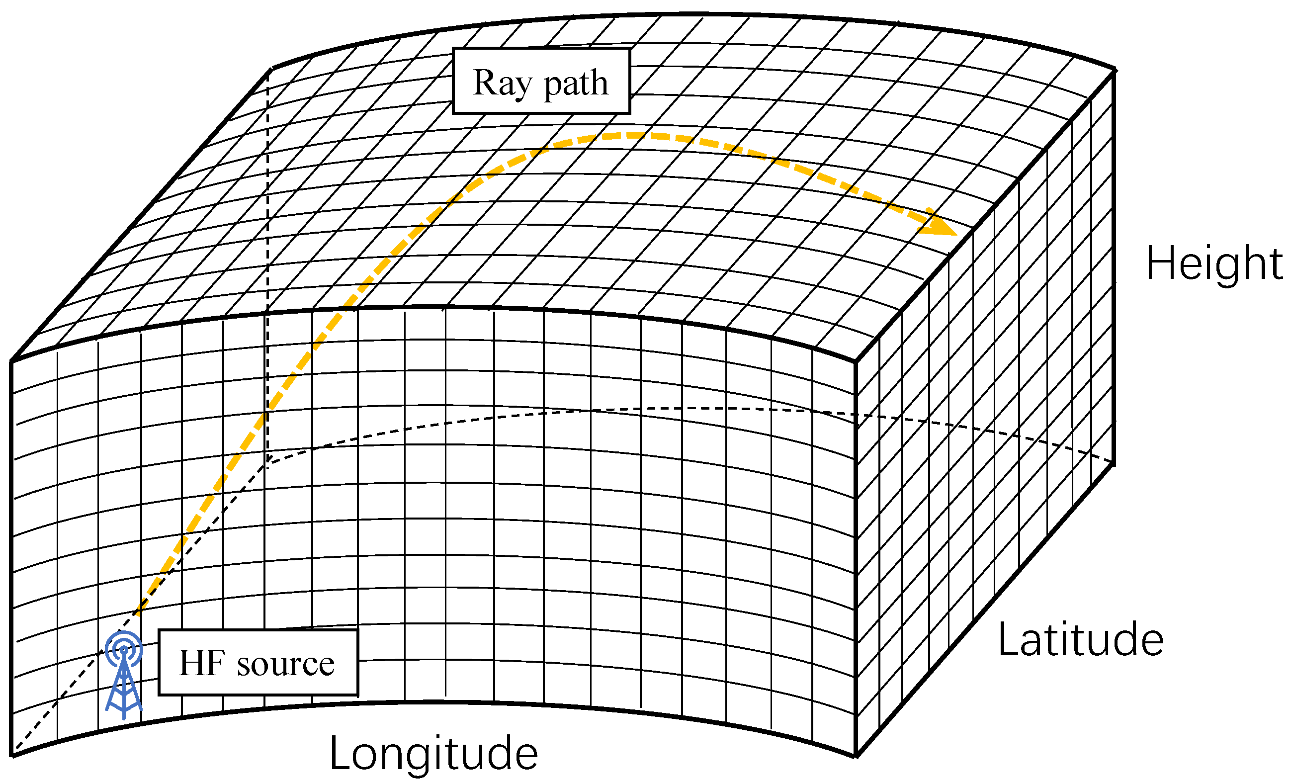
We use the ray tracing method and introduce a realistic ionospheric 3D electron density gridded matrix model to simulate HF signal propagation paths. A detailed explanation of the 3D ionospheric model is given in
Appendix A. The 3D gridded matrix model of the ionosphere electron density is at altitudes ranging from 0 to 1000 km. The gridded matrix elements properties of the ionospheric propagation medium are specified using the Internation Reference Ionosphere (IRI) model with the grid accuracy of
(
). The applicability and limitations of the IRI model are discussed in
Appendix A. We use the methods in [
23] to generate the received signals. For each link, the optimal weights should be set according to its NLOS bias. Since the HF signal propagation paths are unknown in practice, the weight elements
are all set to 1 to reduce the complexity of the problem [
8]. Previous studies show such an approximation does not degrade the performance significantly [
24]. The penalization factor is set as
, and
is set as 1 [
25]. In addition, the proposed method is implemented by the CVX toolbox in MATLAB [
26,
27]. All the simulations are carried out on a computer with 32 GB memory and a 5.0 GHz CPU (Intel Core i7-12700K). The proposed method is compared with the existing geolocation methods: (1) The method proposed in [
12] which maximizes the crosscorrelation function to estimate TDOAs in the first step and derives the target location based on Kalman particle filtering, denoted by KPF. (2) The method proposed in [
13] is based on TDOA Quasi-Parabolic mode, denoted by TQP.
To test the performance of the proposed method, simulations with 100 independent trials are conducted. We calculate the mean square error (MSE) of the estimated position with the Euclidean distance as follows:
where
denotes the real position of the HF source, and
is the estimated position of the HF source at the
independent trial. Moreover, the Cramer–Rao lower bound (CRLB) for TDOA systems in NLOS conditions [
28] is used as the performance benchmark.
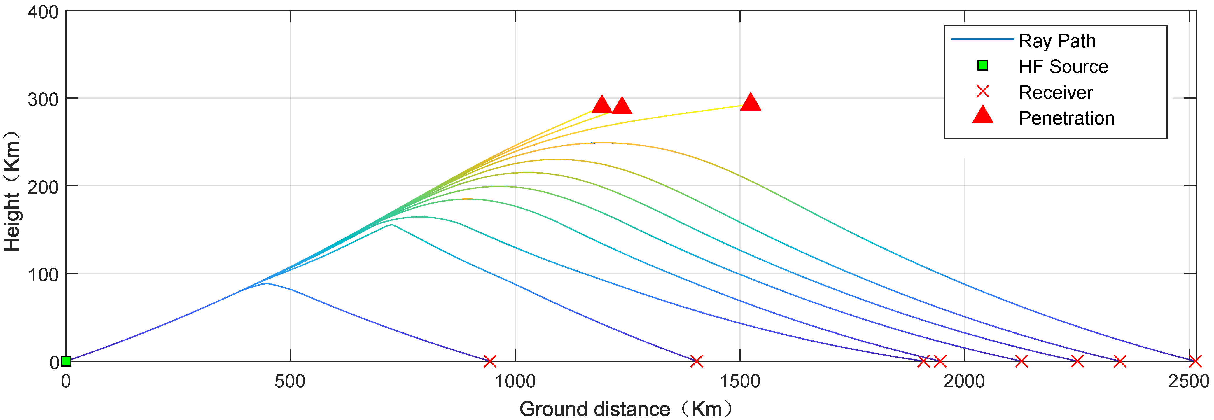
First, we test the performance of the proposed method and compare it with other methods. The HF signal frequency is set to 7.23 MHz. The time of the IRI model is set at 9:00 UT on 13 May 2020.
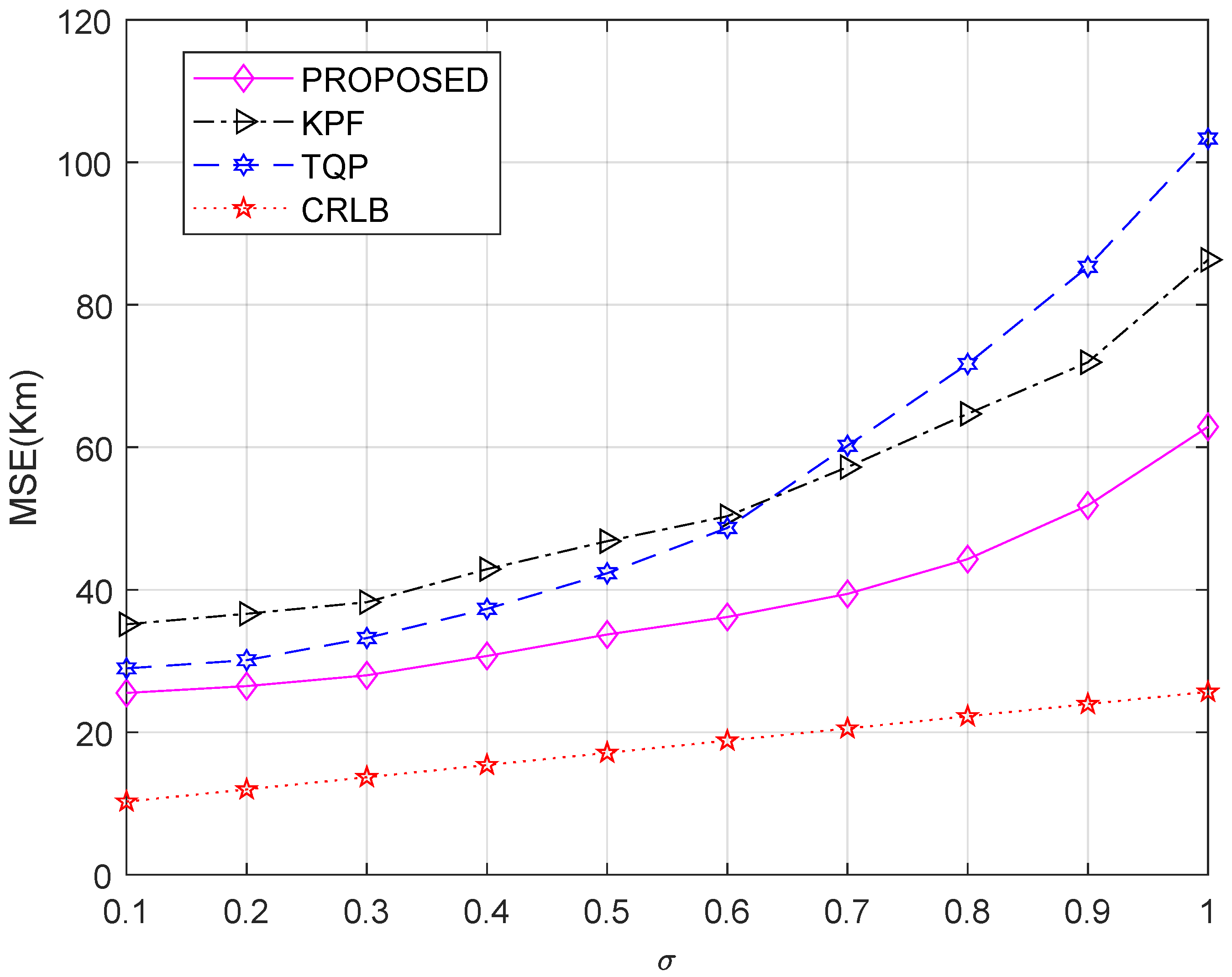
Figure 3 shows the performance comparison with 100 independent geolocation trials of the proposed method and other methods using six receivers in different
conditions. As
increases from 0.1 to 0.5, the proposed method is slightly better than the others. When
, indicating a large measurement noise, the MSEs and interference immunity of the proposed method are significantly better than the other methods.
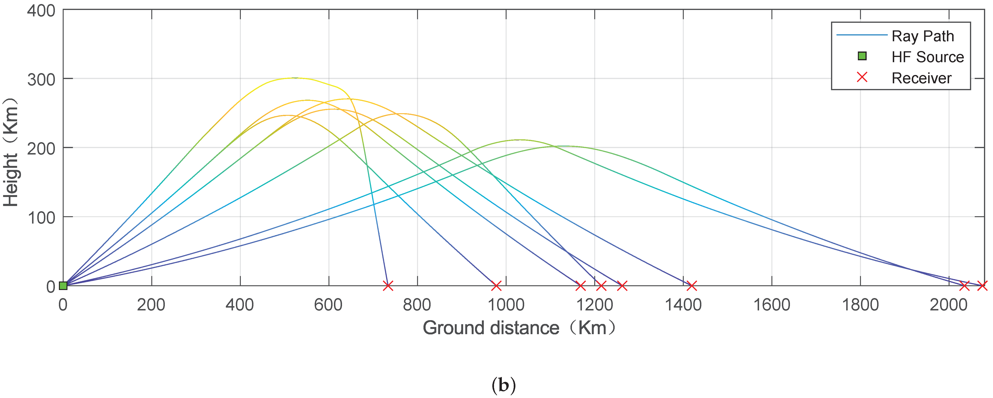
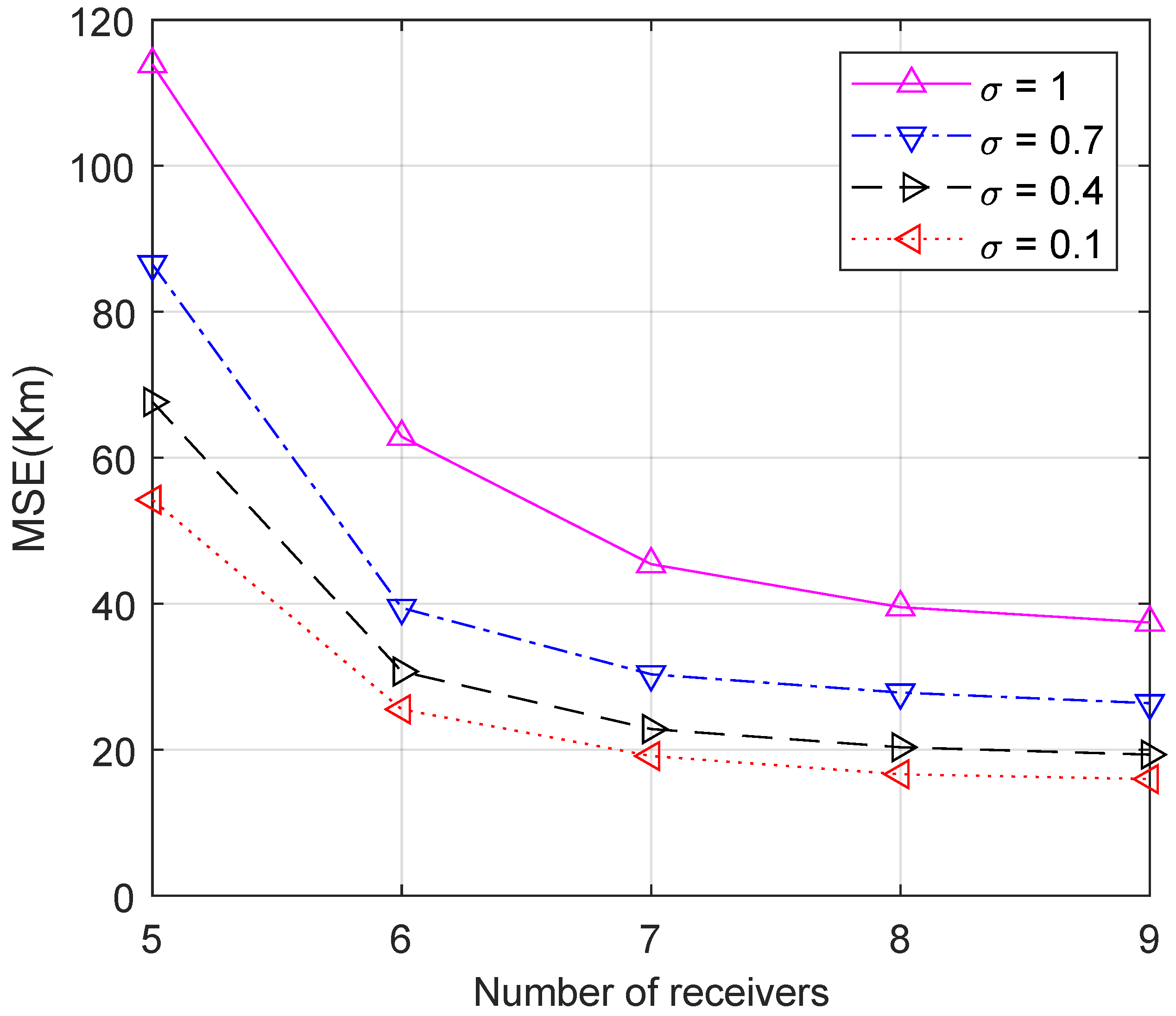
Figure 4 shows the performance with different numbers of receivers and different
. Limited by the number of unknown variables, the proposed method cannot achieve better results when the number of receivers is less than 6 (
). When
, the error decreases and tends to the limit as the number of receivers increases.
Figure 3 and
Figure 4 illustrate that the proposed method outperforms existing algorithms in terms of geolocation accuracy under the same conditions and can significantly suppress the effect of large noise.
Next, we test the performance of the proposed method in the daytime and nighttime in different seasons. The IRI model is set to the 1st of every month, 03:00 UT for the day, and 15:00 UT for the night.
Figure 5 shows the MSE of HF source position estimation in the daytime and nighttime in different seasons. From
Figure 5, the MSEs are slightly higher in summer than in winter and slightly higher in the day than at night due to the influence of ionospheric properties. Unfortunately, due to the IRI model’s limitations, it is impossible to simulate the perturbed ionosphere or ionospheric irregularities. However, the proposed algorithm has good robustness in the simulation.
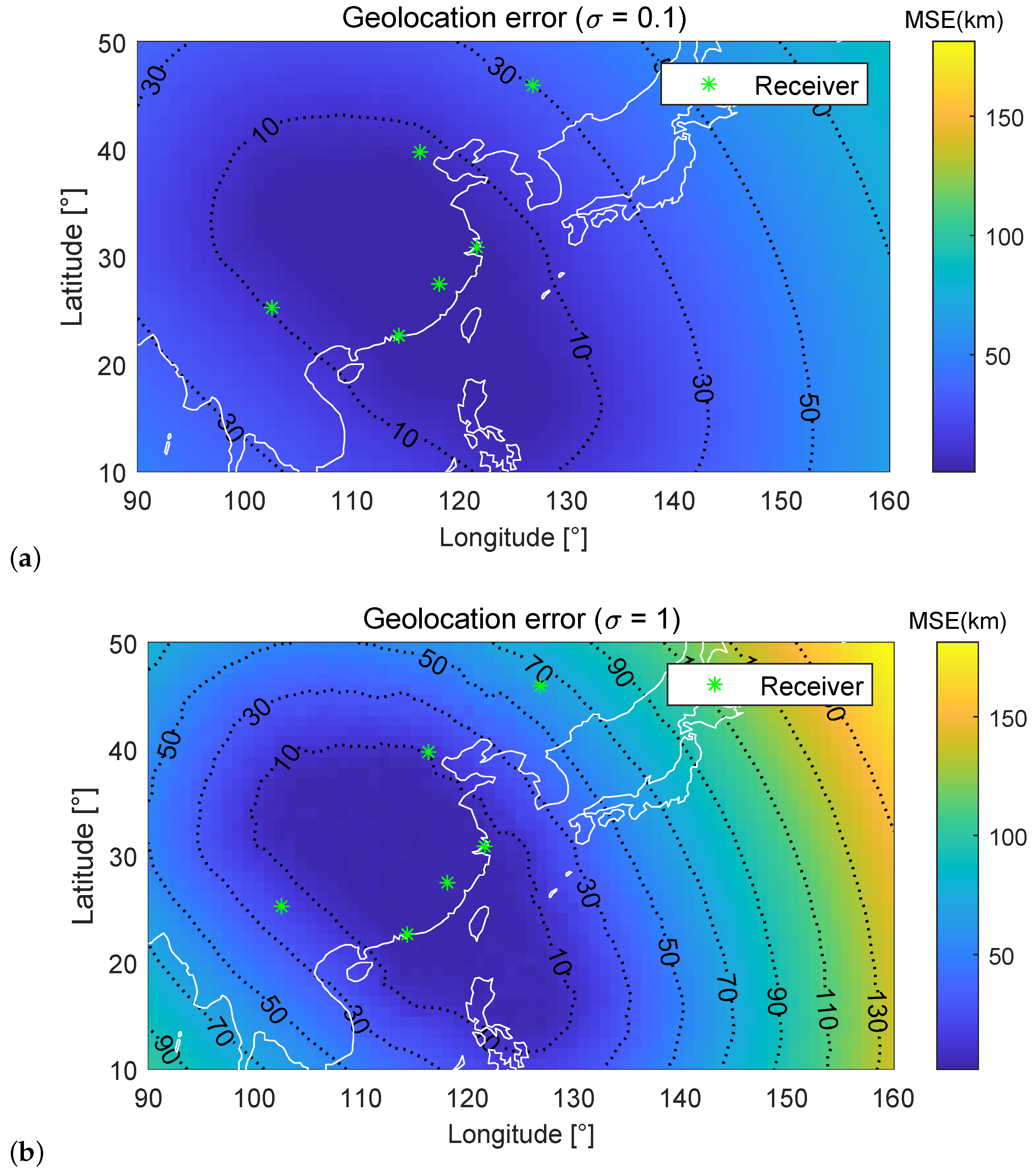
The station arrangement of receivers also significantly affects the accuracy of HF source geolocation. We test two different sets of receiver deployment locations to simulate the real scenario. The first set of six fixed receivers is located in Shenzhen, Beijing, Harbin, Kunming, Shanghai, and Wuyishan, and the time of the IRI model is set at 9:00 UT on 13 May 2020. The second set of six fixed receivers is located in Beijing, Chengdu, Shannxi, Shenzhen, Kunming, and Wuyishan, and the time of the IRI model is set at 15:00 UT on 8 September 2021.
Figure 6 and
Figure 7 show the geolocation error (in km) distribution of the first and second set of 6 fixed receivers under
and
, respectively. Positions of six receivers are marked with asterisks. In
Figure 6 and
Figure 7, the simulation region is divided into grids with an accuracy of
(
). The geolocation error of the HF source at each grid is tested individually, resulting in an error distribution of the entire region. Different receiver arrangement locations result in different geolocation error distributions. For example, when
, the area with MSE < 10 km is
for the first set of six receivers, while the area with MSE < 10 km is
for the second set. However, geolocation error is generally proportional to the distance between the HF source and the receivers.
Table 1 and
Table 2 give the percentage of the different MSE area under
and
. In
Figure 6 and
Figure 7, subject to different levels of noise,
Figure 6a and
Figure 7a are smoother compared to
Figure 6b and
Figure 7b, respectively. It is noteworthy that the increase in noise has a minor impact on the blue region, also called the high-precision region, and a more significant impact on the orange region. When reducing the number of receivers, the high-precision region decreases, and the orange region increases sharply. This phenomenon is consistent with the optimization logic of the algorithm under the antenna deployment position. A good receiver deployment location can significantly improve the geolocation accuracy of HF sources in a specific area and minimize the search and rescue range.
Table 3 gives the running time of the proposed method for a single localization with the different number of receivers.
4.2. Experimental Setup and Results
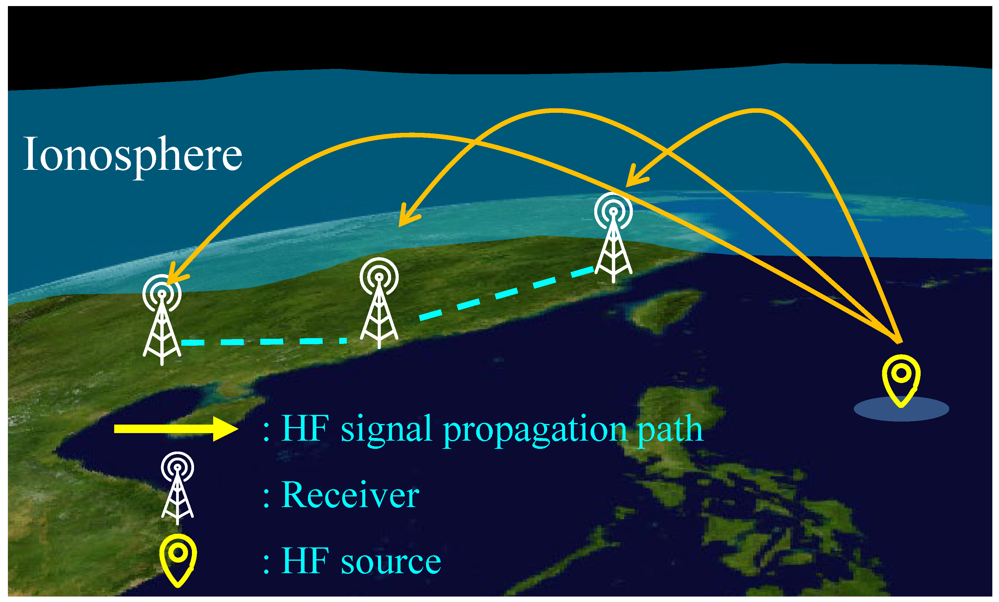
To further demonstrate the effectiveness of our algorithm in real-world scenarios, we use six shortwave signal receivers with GPS time synchronization to build a HF geolocation test system. In the experiment, the receivers capture the target signal synchronously through baseband I/Q sampling. Then, the I/Q data are processed for time difference estimation. The receivers use the Global Positioning System (GPS) and BeiDou Navigation Satellite System (BDS) timing clock to achieve strict synchronization of receivers time. The accuracy of the civilian GPS/BDS timing system is about 50–100 ns, which translates to a distance of about 15–30 m and does not affect the positioning algorithm [
29].
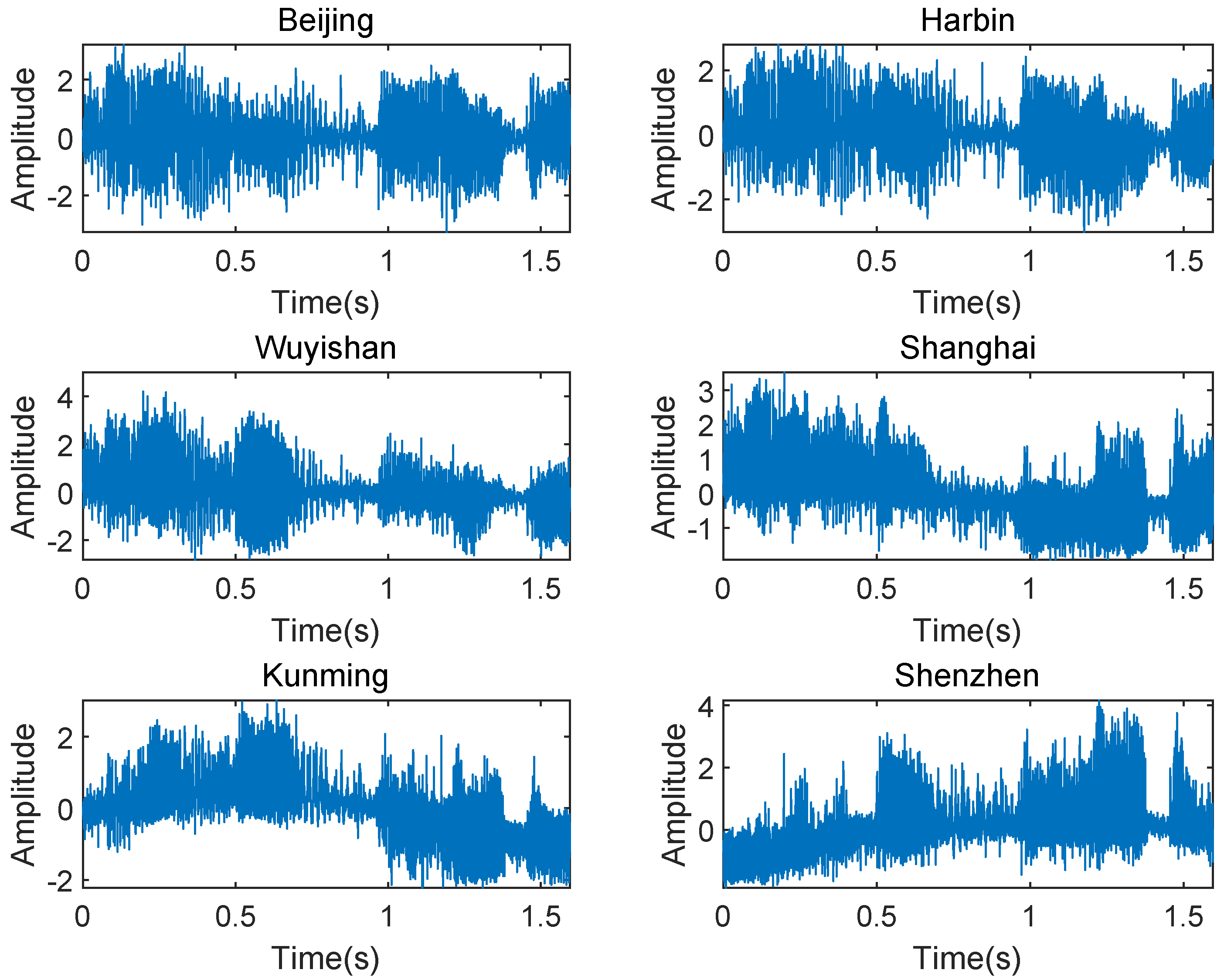
We first verify the capability of locating an AM broadcast signal as shown in
Figure 8. The HF source is located in Xi’an (
). The six fixed receivers are located in Beijing, Harbin, Wuyishan, Shanghai, Kunming, and Shenzhen. The received amplitude modulation (AM) signals captured at 9:15 UTC on 13 May 2020 have a center frequency of 7.23 MHz, a bandwidth of 5 kHz, a sampling rate of 10,240 Hz, and a duration of 1.6 s. The receiver located in Beijing is used as a reference.
Table 4 shows the time delay estimation (TDE) obtained by the AM I/Q data of each receiver.
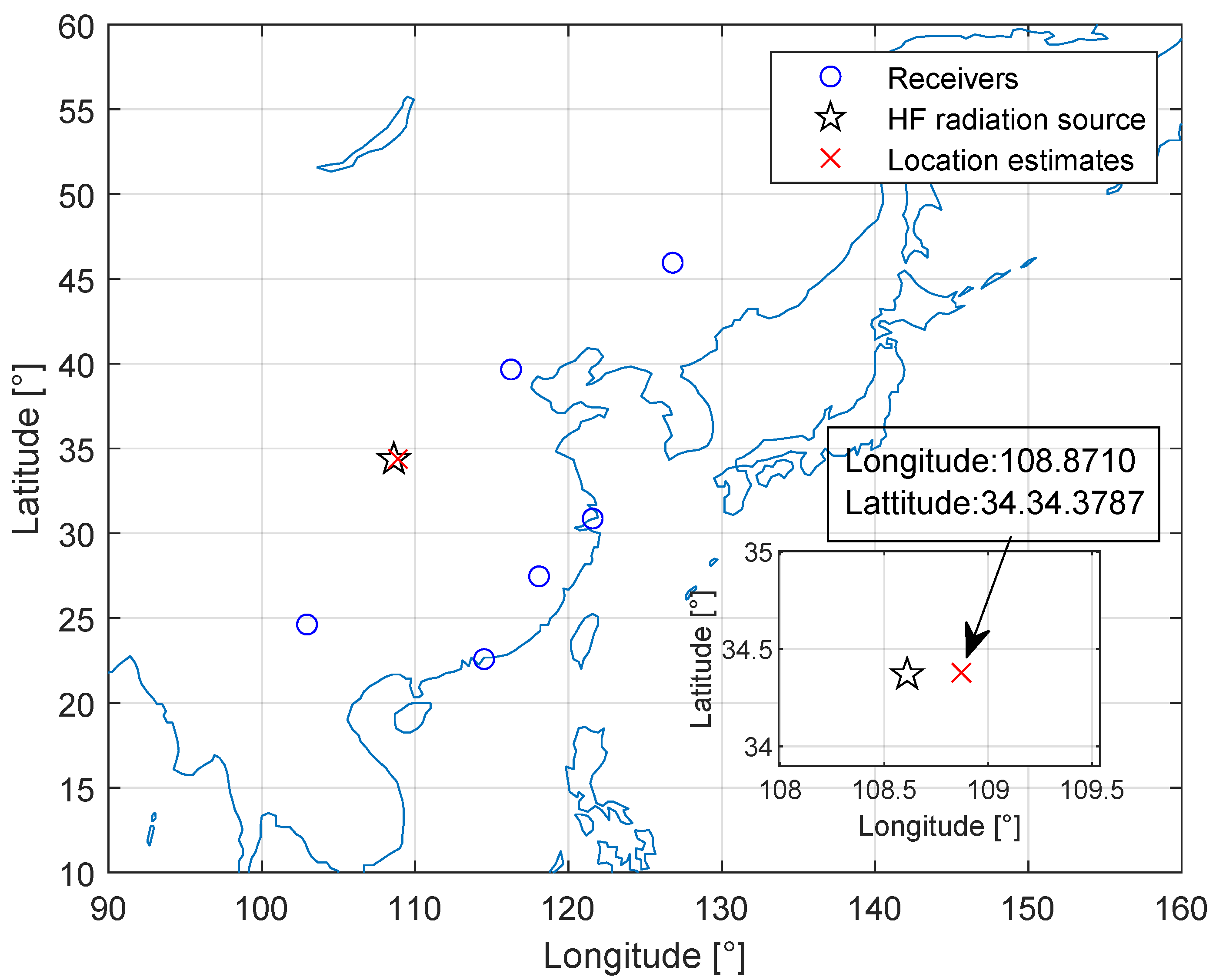
Figure 9 shows the experimental result of Xi’an HF source geolocation estimation. The geographic locations of the receivers (marked with blue circles), the HF source (marked with a black star), and the estimated HF source (marked with a red cross) are shown in
Figure 9. The geolocation error of the HF source is 23.97 km using the proposed method and the relative error is about 0.76%, calculated from dividing the absolute error by the maximum ground range from Harbin to Kunming [
12], which is 3156.34 km.
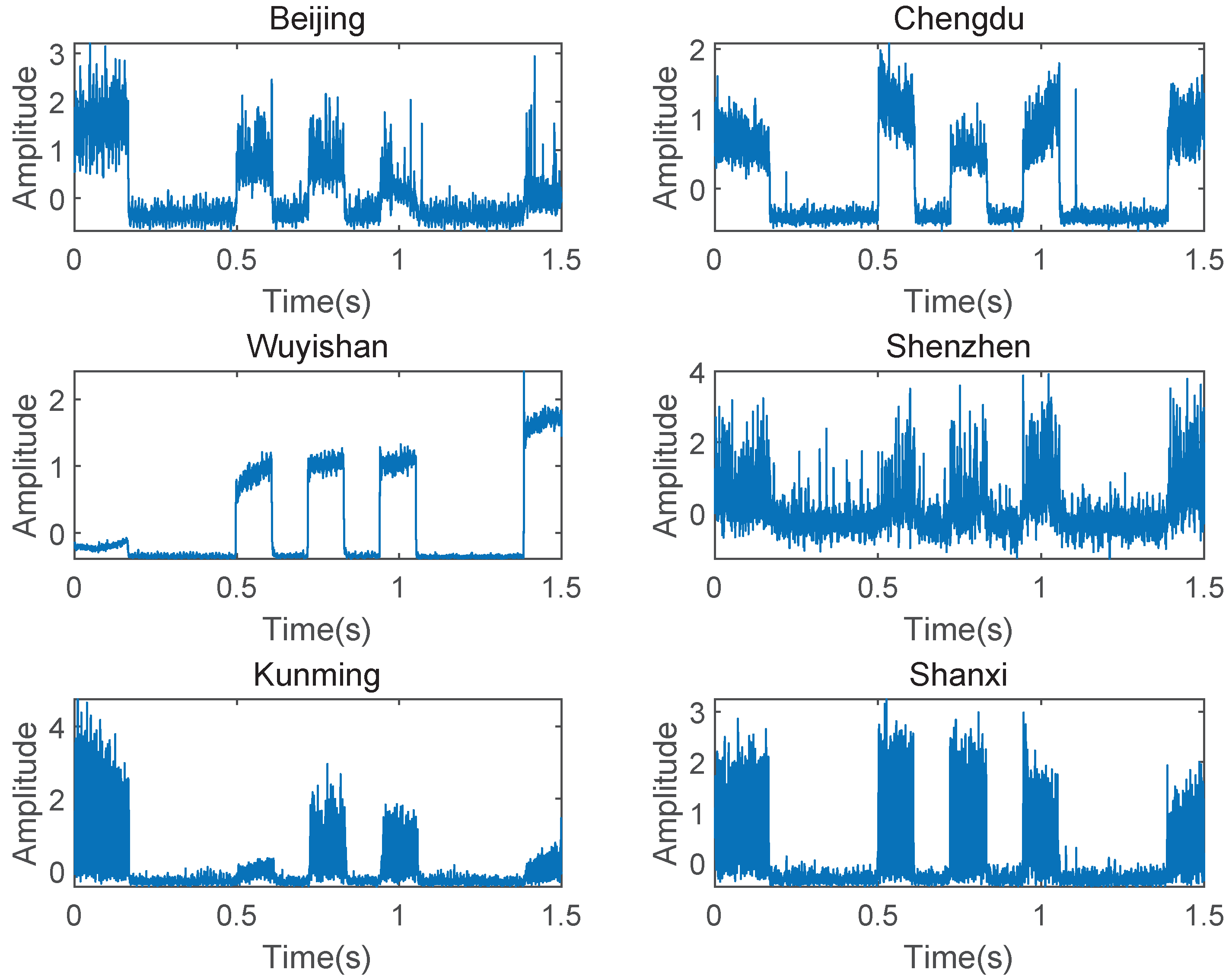
Then, we focus on a frequency shift keying (FSK) signal captured at 15:01 UTC on 8 September 2021 with the center frequency of 8.433 MHz over a 1.5 kHz band, a sampling rate of 8152 Hz, and a duration of 1.5 s, as shown in
Figure 10. The FSK modulated signal is used by a coast radio station, which is located in Shanghai (
). The six fixed receivers are located in Beijing, Chengdu, Shannxi, Shenzhen, Kunming, and Wuyishan. The receiver located in Wuyishan is used as a reference.
Table 5 shows the TDE obtained by the FSK I/Q data of each receiver.
The estimated Shanghai HF source (marked with a red plus marker) is shown in
Figure 11. The geolocation error of the HF source is 33.65 km using the proposed method, and the relative error is about 1.61%, calculated from dividing the absolute error by the maximum ground range from Beijing to Kunming, which is 2084.56 km.
Finally, we assess all the sampled data in the time period in which AM and FSK are located, with a duration of 1.5 s for each set of data and an interval of 8.5 s between each measurement. As shown in
Table 6, we summarize the maximum error and minimum error of the three geolocation methods. The average relative error of the proposed method is less than 2.7%, which improves the geolocation performance by about 50% compared with other methods. Under the same conditions, the proposed method has better noise immunity and the geolocation capability than other methods.


