An Investigation of Signal Preprocessing for Photoacoustic Tomography

Huen, Isaac; Zhang, Ruochong; Bi, Renzhe; Li, Xiuting; Moothanchery, Mohesh; Olivo, Malini

doi:10.3390/s23010510

Open AccessArticle

An Investigation of Signal Preprocessing for Photoacoustic Tomography

by

Isaac Huen

,

Ruochong Zhang

,

Renzhe Bi

^*

,

Xiuting Li

,

Mohesh Moothanchery

and

Malini Olivo

Institute of Bioengineering and Bioimaging, A*STAR, 11 Biopolis Way, Singapore 639798, Singapore

^*

Author to whom correspondence should be addressed.

Sensors 2023, 23(1), 510; https://doi.org/10.3390/s23010510

Submission received: 31 October 2022 / Revised: 7 December 2022 / Accepted: 21 December 2022 / Published: 2 January 2023

(This article belongs to the Special Issue Theory and Applications of Photoacoustic Imaging and Sensing)

Download

Browse Figures

Versions Notes

Abstract

:

Photoacoustic tomography (PAT) is increasingly being used for high-resolution biological imaging at depth. Signal-to-noise ratios and resolution are the main factors that determine image quality. Various reconstruction algorithms have been proposed and applied to reduce noise and enhance resolution, but the efficacy of signal preprocessing methods which also affect image quality, are seldom discussed. We, therefore, compared common preprocessing techniques, namely bandpass filters, wavelet denoising, empirical mode decomposition, and singular value decomposition. Each was compared with and without accounting for sensor directivity. The denoising performance was evaluated with the contrast-to-noise ratio (CNR), and the resolution was calculated as the full width at half maximum (FWHM) in both the lateral and axial directions. In the phantom experiment, counting in directivity was found to significantly reduce noise, outperforming other methods. Irrespective of directivity, the best performing methods for denoising were bandpass, unfiltered, SVD, wavelet, and EMD, in that order. Only bandpass filtering consistently yielded improvements. Significant improvements in the lateral resolution were observed using directivity in two out of three acquisitions. This study investigated the advantages and disadvantages of different preprocessing methods and may help to determine better practices in PAT reconstruction.

Keywords:

photoacoustic tomography; preprocessing; wavelet denoising; CNR; resolution

1. Introduction

Photoacoustic or optoacoustic tomography (PAT) is an emerging modality that combines the high contrast of optical methods and good resolution in deep tissue with acoustic detection. Being able to break through the optical diffusion limit, PAT has shown great potential in the noninvasive detection of early-stage cancer [1] and the imaging of the brain [2]. When tissue is illuminated with a modulated light source, it absorbs energy followed by periodic thermal expansion to generate an ultrasonic wave. A transducer is employed to collect the propagated ultrasonic wave, which forms the final image by reconstruction. The signal-to-noise ratio (SNR) of the received PA signal is limited by several factors. First of all, the efficiency at each stage of energy conversion is not 100%, accompanied by additional thermal noise, electronic noise, etc. Moreover, in PAT, a high-power nanosecond pulsed laser is usually adopted to illuminate an area of tissue, and the amplitude of the generated PA signal in MHz is largely dependent on the optical absorption of the target. However, according to ANSI standards [3], there is a maximum permissible exposure (MPE) of lasers on human skin, which limits the excitation energy delivered into tissue and the strength of the generated signal. Because of these factors, the received PA signal could be weak and noisy, which may affect the final image quality, especially in deep tissue.

There are several preprocessing methods to enhance the raw PA signal before reconstruction. Excluded from this consideration is the averaging of multiple acquisitions, as increased acquisition time may affect the imaging of tissue motion. A signal is typically decomposed into components (the basis functions characterized by coefficients), with differences between the signal and noise coefficients allowing for the removal of noise. The Fourier transform method uses a simple basic function, the sinusoid, characterized by its frequency [4]. Hence lowpass, bandpass, and matched filters exclude noise-dominated frequencies, although this could also result in a signal loss if it occupies the same frequencies [5,6].

Improved results could be obtained by changing the basis function to waveforms matched to the signal, as in wavelet denoising [7,8]. The signal is decomposed using the discrete wavelet transform method into wavelet coefficients where, ideally, the signal and noise are separated. These noise coefficients are then removed based on thresholds, and the pure signal is reconstructed using the inverse wavelet transform method. This approach was demonstrated to yield SNR improvements in many applications, including chick embryos and rat brains [9], as well as in photoacoustic microscopy in melanoma cells [10]. It was shown to outperform both lowpass and bandpass filters, with bipolar “Symlet” family wavelets found most effective both in silico and in vivo, although the parameters depended on the frequency content and SNR of the image [7].

Empirical mode decomposition (EMD) sifts (decomposes) signals into intrinsic mode functions (IMFs), which have the advantage of being able to vary in frequency and amplitude. Feature selection is then used to identify noisy IMFs and remove them. This was previously demonstrated to improve photoacoustic images in several studies, including a simple approach of merely including the first two IMFs [11,12,13].

Singular value decomposition (SVD) was also used to remove laser-induced noise in photoacoustic images [11]. This is based on decomposing the imaging operator H, which is responsible for noise, into its component matrices USV^T, where S is a diagonal matrix containing the singular values of each component. Noisier components could then be removed; indeed, better performance was achieved using just a single component [10].

It is also of relevance that sensors are not omnidirectional but less sensitive in particular directions [14]. The noise-related artefacts resulting from this were illustrated with simulations to date, including using the MATLAB k-wave toolbox [15] and Monte Carlo simulation of red blood cell signals, demonstrating a fourfold increase in accuracy when reconstruction accounted for sensor directivity, according to [16].

However, to our knowledge, there has not been a detailed comparison of the combinations of common preprocessing methods, and thus an optimal preprocessing workflow has not yet been defined. Non-classical methods, such as deep learning, were demonstrated for noise reduction, object detection, and segmentation [17]. However, these are not suitable for inclusion in the comparison because they are not a well-defined algorithm but are trained to datasets, which are typically simulated with limited translatability to experimental datasets [18]. We, therefore, restricted the scope of comparison to common classical methods.

In this paper, we aimed to investigate and optimize the preprocessing of PA signals from a 256-element multi-segment transducer [19] by comparing the reconstructed 2D PA image quality of the combinations of the unfiltered signal, bandpass filter, deconvolution, wavelet denoising, and sensor directivity. We used the metrics of noise reduction (measured as the contrast-to-noise ratio [CNR]) and resolution in both directions (measured as FWHM) to quantify the performance of each combination. These were investigated in a range of acquisitions from single-point sources, to multiple-point sources and finger imaging.

2. Materials and Methods

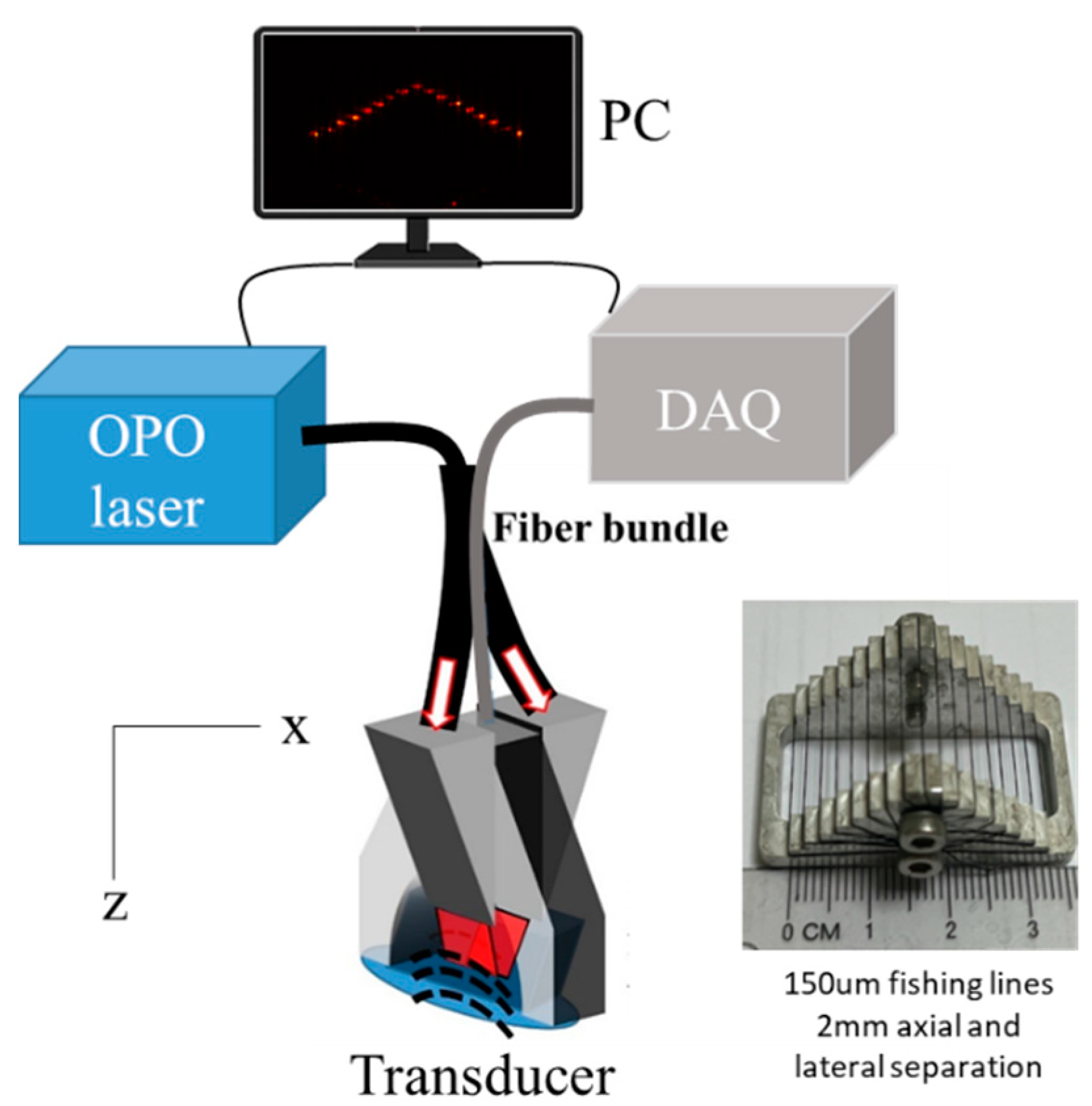
2.1. Image Acquisition

A 20 Hz tunable optical parametric oscillator (OPO, Ekspla) nanosecond pulsed laser was shone through a fiber bundle from one side of the transducer to illuminate the sample. The output energy at 700 nm was fixed at 45 mJ with a 3 cm² illumination area, corresponding to a fluence of ~15 mJ/cm². A customized multi-segment transducer with 256 elements arranged in an arc-linear-arc shape was used to acquire the PA data, as described in [19]. The sampling rate of the data acquisition unit (DAQ) was set to 40 MHz, and 3072 points were acquired for each channel. A PC was used to control the software written in MATLAB and save the data. In the phantom experiments, a 150 µm black fishing line was imaged first (“point” acquisition). A phantom composed of 17 fishing lines arranged in a pyramid shape was also used, as shown in Figure 1 (“multi-point” acquisition). This consisted of 1 point at the top, with 8 rows of increasing lateral separation below. The axial and lateral separation between successive points was 2 mm. Moreover, imaging on a finger was also performed (“finger acquisition”).

2.2. Signal Processing

All image processing was carried out in MATLAB R2019b. The signal processing workflow for all compared methods is shown in Figure 2. The parameters for all methods are shown in Table 1.

The sensor signal underwent a bandpass filter, wavelet denoising, EMD, or SVD, or was unfiltered, followed by applying directivity or not. This yielded 10 combinations (unfiltered, bandpass, wavelet, EMD, SVD, unfiltered+directivity, bandpass+directivity, wavelet+directivity, EMD+directivity, SVD+directivity).

2.2.1. Optimization of Preprocessing Methods’ Parameters

The bandpass filter’s FWHM was set at 90% of the central frequency.

The wavelet denoising parameters (wavelet family, order, denoising method, threshold rule, and noise estimation) were optimized with CNR maximization and the minimization of FWHM_x and FWHM_z (Appendix A). It was found that the wavelets of the Daubechies family performed best in the fourth order. The optimized values of all parameters are listed in Table 1.

EMD was performed using the MATLAB emd function by iteratively decomposing the data X(t) into IMFs and a residual. This involved the following steps [20,21]:

Finding all local minima and maxima of the data;
The calculation of the lower and upper envelopes by the cubic spline interpolation of the minima and maxima, respectively;
Calculating the mean of the lower and upper envelopes, $m_{1}$ ;
Calculating the provisional component h₁ as the difference between the data and $m_{1}$ : $h_{1} = X (t) - m_{1}$ ;
Repeat sifting (steps 1–4) but using the provisional component as the data, yielding $h_{11} = h_{1} - m_{11}$ ;
Continue sifting k times until the stopping criterion is reached, yielding $h_{1 k} = h_{1 (k - 1)} - m_{1}$ . This is the first component, $c_{1}$ ;
Derive the residue $r_{1}$ : $r_{1} = X (t) - c_{1}$ ;
Repeat steps 1–8 using the residue r₁ as the data, yielding $c_{2} = r_{1} - r_{2}$ ;
Continue repeating steps 1–8 to yield all further components: $c_{n} = r_{n - 1} - r_{n}$ ;
Stop when the residue $r_{n}$ is a monotonic function, meaning no more minima and maxima exist, and thus no more components are extracted.

This was followed by summing the first two components and taking their absolute value.

SVD was performed using the MATLAB svd function to decompose the data matrix X of dimension n × p (where n is the number of sensors and p is the number of time points) into a matrix of left vectors U of the dimension n × n, a diagonal singular value matrix S of the dimension n × p, and a matrix of right vectors V of the dimension p × p.

X = U S V^{T}

As previously demonstrated, this decomposition characterized the laser-induced noise in particular because the noise was consistent across sensors, and using one singular value component was sufficient [10]. Therefore, all values in S except the first diagonal value were set to zero to form the laser-induced singular value matrix S_L. The noise was then calculated as US_LV^T and subtracted from the original signal X.

After these preprocessing steps were completed, the universal back-projection algorithm [22] was used for image reconstruction.

2.2.2. CNR Measurement

CNR could be defined in the following way [23]:

CNR=|S_I−S_o|/σ_o

(1)

where S_I and S_o are the means of the ROIs located inside and outside the signal of interest, respectively, and σ_o is the standard deviation of the ROI located outside.

A signal ROI of 20-pixel half-width was drawn centered on the pixel with the maximum signal. S_I was thus the mean of this region. A noise ROI of 50-pixel half-width was drawn in the top left of the image, away from the signal or artefact. The S_noise and σ_noise were the mean and standard deviation of this ROI, respectively. We then calculated the CNR = |S_I−S_noise|/σ_noise.

As another indicator of image quality, we also calculated the peak SNR where:

Peak SNR= S_Imax/σ_o

(2)

where S_Imax is the maximum value of the signal ROI, and σ_o is the standard deviation of the noise ROI.

2.2.3. Resolution Measurement

FWHM_x and FWHM_z were used to represent the lateral and axial resolution of the reconstructed image. The FWHM_x measurements were performed inside the signal ROI centered on the pixel with the maximum signal identified in 2.2.2. The signal was taken from a range of x-coordinates 20 pixels below and above this pixel, yielding 41 points in total. Its minimum was subtracted to eliminate the need to fit a constant as an additional parameter. This was then fitted to a three-term Lorentzian function (using the lorentzfit function from MATLAB Central) to yield its scale parameter γ. This was multiplied by 2 to yield FWHM_x. The analogous procedure was repeated in the z-direction to yield FWHM_z. Since these were in units of pixels, they were converted to μm via multiplication by the x- and z-resolutions.

The multi-point acquisition had a range of intensities at different points, and we, therefore, needed to select a single measurement for comparison. We compared the CNR and resolution measurements for every point using the default unfiltered method (Appendix B). The best results were obtained in the middle row (Appendix B), and thus, the CNR and resolution results were reported as the average of the pair of points in this row.

The results were reported as CNR, FWHM_x, and FWHM_z. The changes relative to the control (unfiltered) method were reported as ΔCNR, ΔFWHM_x, and ΔFWHM_z.

3. Results

Whole images are shown, for example, the methods in the point, multi-point, and finger acquisitions (Figure 3) with the noise ROI annotated.

The CNR and FWHM measurements are shown in Table 2. A higher CNR represents better noise reduction, while a lower FWHM represents better resolution. Comparisons with the actual imaging phantom were listed in the brackets under the FWHM columns. The changes relative to the unfiltered method were calculated for all measurements (ΔCNR, ΔFWHM_x, and ΔFWHM_z) in Figure 4.

The unfiltered+directivity method had the highest ΔCNR in two of three acquisitions, with bandpass+directivity being second and highest in the other. Averaged across all three acquisitions, bandpass+directivity had the highest ΔCNR, unfiltered+directivity was second, SVD+directivity was third, wavelet+directivity was fourth, and EMD+directivity was last. For the non-directivity methods, the same order resulted. The CNR of the directivity methods was significantly higher than the non-directivity methods (paired t-test, p < 0.05) for all three acquisitions.

There were various trends for FWHM. The five largest FWHM_x decreases occurred using the five directivity methods in the point acquisition. In the multi-point acquisition, five of the six largest FWHM_z increases were from the directivity methods. The FWHM_x of the directivity methods was significantly lower than the non-directivity methods (paired t-test, p < 0.05) in all acquisitions except for the multi-point acquisition.

4. Discussion

The use of directivity significantly improved noise reduction in all acquisitions. Though it significantly improved lateral resolution in two of the acquisitions, its effects on the resolution were mixed. There appeared to be two main effects of directivity: reductions in the intensity of the streaks broadly from the top-left to the bottom-right direction (green markers, Figure 3A vs 3P, Figure 3K vs 3Z), which is closest to the lateral direction and thus likely measured as an improvement of lateral resolution. They also reduced the noise (measured in the yellow box), resulting in the observed increase in the CNR. There are also increases in the streak length broadly from the top-right to the bottom-left direction (blue markers, Figure 3A vs 3P, Figure 3K vs 3Z), which is closest to the axial direction and thus likely measured as a worsening of axial resolution. The magnitude of the measured effects depended on how lateral the signal ROI was from the sensor array. This was relatively central in the point and finger acquisitions but more lateral in the multi-point acquisition because it was in the middle row. Considerable variations in streak lengths are seen at different locations using directivity in the multi-point acquisition (yellow marker, Figure 3U), which may be why the multi-point acquisition lacked a significant improvement in lateral resolution.

Adding directivity caused larger improvement in noise reduction, and to some extent, resolution, than different preprocessing methods. This is shown by the five largest axial resolution improvements occurring using the five directivity methods in the point acquisition and being significantly lower in all acquisitions except the multi-point acquisition, where, as suggested, the behavior is different due to the lateral signal ROI positioning. Even here, five of the highest six reductions in the axial resolution are from directivity methods, showing that directivity has a more significant effect.

The order of noise reduction is the same both with and without directivity. In decreasing order, it is: bandpass, unfiltered, SVD, wavelet denoising and EMD. Wavelet denoising had its best values for noise reduction, lateral resolution, and axial resolution only in the acquisition it was optimized for, the point acquisition, which suggests it is not generally optimized. This is supported by the noise reduction and lateral resolution becoming progressively worse with the increasing complexity of the signal, moving from the point to multi-point and finger acquisitions. Bandpass appeared to offer moderate improvements in noise reduction without much cost to the resolution and was the only method to outperform the unfiltered method consistently. Inconsistent results for lateral resolution were obtained using EMD and SVD. Distinctive artefacts are seen in the point acquisition (red markers, Figure 3D and 3E).

While this paper sought to provide a comparison of the common preprocessing methods and not the algorithm for deployment itself, we note the calculation time was, depending on the method, 7 to 43 s for a high-resolution (1200 × 1200) image. While this is below the speed required for real-time imaging, this could be achieved using parallelization and GPU acceleration which have previously yielded acceleration factors of 140-fold [24] and 125- to 1000-fold [25].

Deep learning methods were also used for preprocessing, such as the usage of convolutional neural networks (CNNs) [26] for artefact removal, the extension of bandwidth, and object detection using region-based CNNs [27,28,29] to separate signals from artefacts. While these could yield impressive results in terms of noise reduction, they are limited by the need for ground truth upon which to train, such as anatomical markers. This is typically difficult to obtain, resulting in the use of simulated data by a majority of studies which have shown poor translation to experimental data [18]. This ultimately limits the reliability of images for pathology and hence clinical diagnoses. As a black box, they generally are unable to show the paper trail of how the image was derived.

Furthermore, we note that this work was only focused on established preprocessing methods from a practical point of view demonstrated directly by experiments. The results may be affected by different experimental conditions such as laser fluence, transducer performance, target absorption, etc. Analytical models [30,31,32] may be helpful in predicting, verifying, and generalizing the results.

5. Conclusions

In conclusion, we tested combinations of classical signal preprocessing methods and directivity for 2D PA image reconstruction and found that directivity yields considerable improvements in both noise reduction and lateral resolution with the multi-segment transducer. With and without directivity, only bandpass filtering consistently yielded an improvement. Moreover, the advantages and disadvantages of other preprocessing methods were also investigated, which may be helpful in determining better preprocessing practices in PAT reconstruction.

Author Contributions

Conceptualization, R.B.; software, I.H., R.Z. and X.L.; software, R.Z. and M.M.; validation, I.H.; formal analysis, I.H.; resources, R.B. and M.O.; writing—original draft preparation, I.H.; writing—review and editing, R.Z. and X.L.; supervision, R.B. and M.O.; All authors have read and agreed to the published version of the manuscript.

Funding

This work was supported by (1) Agency of Science, Technology and Research (A*STAR), under its BMRC Central Research Fund (UIBR) 2021 and (2) Horizontal Technology Programme Office Seed Fund, Biomedical Engineering Programme 2021, C211318004.

Institutional Review Board Statement

Not applicable.

Informed Consent Statement

Not applicable.

Data Availability Statement

Data will be provided upon reasonable request.

Conflicts of Interest

The authors declare no conflict of interest. The funders had no role in the design of the study; in the collection, analyses, or interpretation of data; in the writing of the manuscript, or in the decision to publish the results.

Appendix A

Appendix A.1. Optimization of Wavelet Denoising

Wavelet denoising parameters (wavelet family, order, denoising method, threshold rule, and noise estimation) were optimized by the maximization of the CNR and the minimization of FWHM_x and FWHM_z on the point acquisition alone. Image processing was carried out using the default unfiltered method without directivity.

Appendix A.2. Selection of the Wavelet Family and Order

Each wavelet family available in MATLAB was compared (Table A1), namely coif (Coiflets), fk (Fejer-Korovkin), db (Daubechies), sym (Symlet), and haar (Haar). For all except haar, the wavelet orders also needed to be specified. Starting from the lowest order, the orders were tested until the maximum order specifiable was reached, or the CNR was observed to decrease monotonically for at least two orders.

Default settings were used for the other required parameters: “DenoisingMethod” was set to “universal threshold”, “ThresholdRule” was set to “soft”, and “NoiseEstimation” was set to “level-dependent”. However, these settings were optimized in the following two stages.

Table A1. Comparison of the wavelet families and orders.

Family and Order Comparison
Family	Order	CNR	Rank	FWHMx	Rank	FWHMz	Rank	Average Rank	Rank
coif	1	34.27	13	552.1	1	779.8	21	11.7	13
	2	34.74	10	553.07	10	779.54	11	10.3	11
	3	36.28	2	553.98	13	779.43	6	7.0	2
	4	36.03	3	554.46	15	779.46	7	8.3	6
	5	36.84	1	555.25	19	779.38	4	8.0	4
fk	4	33.61	20	554.25	14	779.76	20	18.0	21
	6	33.18	21	555.69	20	779.46	7	16.0	20
	8	34.83	8	553.61	11	779.39	5	8.0	4
db	1	33.65	17	552.56	6	779.68	17	13.3	15
	2	33.73	15	554.86	16	779.56	12	14.3	18
	3	34.36	11	552.51	4	779.67	15	10.0	9
	4	35.42	5	552.38	2	779.35	3	3.3	1
	5	35.15	7	553.63	12	779.2	2	7.0	2
	6	35.19	6	555.06	18	779.16	1	8.3	6
sym	1	33.65	17	552.56	6	779.68	17	13.3	15
	2	33.73	15	554.86	16	779.56	12	14.3	18
	3	34.36	11	552.51	4	779.67	15	10.0	9
	4	34.24	14	552.47	3	779.59	14	10.3	11
	5	35.79	4	556.38	21	779.49	10	11.7	13
	6	34.78	9	552.77	9	779.46	7	8.3	6
haar		33.65	17	552.56	6	779.68	17	13.3	15

The Daubechies family, with the fourth order, was selected as this was the highest-ranked.

Next, all permutations of “DenoisingMethod” and “ThresholdRule” were compared to find the best “ThresholdRule” in each “DenoisingMethod” (Table A2). Since using the absolute rank produced too many ties, the rank of the average % behind the best was used.

Table A2. Comparison of the permutations of “DenoisingMethod” and “ThresholdRule”.

db4 DenoisingMethod and ThresholdRule Comparison
DenoisingMethod	ThresholdRule	CNR	Rank	FWHMx	Rank	FWHMz	Rank	Average % behind Best	Rank
UniversalThreshold	Soft	35.42	11	552.38	12	779.35	1	1.14%	2
	Hard	35.48	10	550.52	1	780.25	5	1.15%	3
Bayes	Median	36.19	5	550.68	3	780.34	8	1.85%	7
	Mean	36.22	4	550.84	5	780.33	7	1.89%	9
	Soft	36.15	6	551.67	9	779.86	3	1.85%	8
	Hard	36.28	3	550.72	4	780.43	12	1.94%	10
Minimax	Soft	35.9	8	551.7	10	779.65	2	1.60%	5
	Hard	36.03	7	550.66	2	780.41	11	1.69%	6
FDR	Hard	35.51	9	550.97	6	780.37	9	1.21%	4
BlockJS	James-Stein	34.34	12	552.09	11	780.27	6	0.13%	1
SURE	Soft	36.48	1	551.22	8	780.17	4	2.15%	12
	Hard	36.29	2	551.12	7	780.4	10	1.97%	11

Finally, each of these combinations was compared using both level-dependent and level-independent noise estimation (Table A3). The highest-ranked combination was used. In total, this was Daubechies fourth order, universal threshold, hard thresholding, and level-dependent noise estimation.

Table A3. Comparison of noise estimation with and without level dependence.

db4 NoiseEstimation Comparison
DenoisingMethod/ ThresholdRule	NoiseEstimation	CNR	Rank	FWHM_x	Rank	FWHM_z	Rank	Average Rank	Rank
UniversalThreshold/hard	LevelDependent	35.48	5	550.52	1	780.25	2	2.67	1
	LevelIndependent	34.09	4	552.22	10	780.29	3	5.67	6
Bayes/median	LevelDependent	36.15	9	551.67	5	779.86	1	5.00	4
	LevelIndependent	34.25	5	552.12	8	780.31	4	5.67	6
Minimax/hard	LevelDependent	36.03	8	550.66	2	780.41	10	6.67	9
	LevelIndependent	33.99	2	552.11	7	780.32	5	4.67	2
FDR/hard	LevelDependent	35.51	7	550.97	3	780.37	8	6.00	8
	LevelIndependent	33.98	1	552.12	8	780.32	5	4.67	2
SURE/hard	LevelDependent	36.29	10	551.12	4	780.4	9	7.67	10
	LevelIndependent	34	3	552.07	6	780.33	7	5.33	5

Appendix B

Selection of the Optimal Row from the Multi-Point Acquisition

For each of the 17 points in the multi-point acquisition, the CNR, FWHM_x, and FWHM_z were individually calculated (Figure A1).

Figure A1. CNR, FWHMx, and FWHMz calculated for each of the 17 points in the multi-point acquisition.

The results (Table A4) were organized into rows, with the first row consisting of one point, followed by eight rows of two points. The average CNR, FWHM_x, and FWHM_z were calculated for each row. It was decided to use row five because it had the best values for the CNR and FWHM_x.

Table A4. Comparison of CNR and resolution for each row in the multi-point acquisition.

	CNR (μm)		FWHM_x (μm)		FWHM_z (μm)
Row	µ	σ	µ	σ	µ	σ
1	7.71	N/A	630.71	N/A	782.56	N/A
2	9.6	0.59	538.2	1.98	786.06	7.58
3	10.89	1.42	541.88	4.47	777.97	0.36
4	11.78	2.5	545.96	7.71	787.91	14.5
5	13.25	1.61	537.6	0.53	783.23	5.37
6	12.28	2.11	583.72	67.04	778.73	2.39
7	10.52	2.62	544.54	7.74	774.52	4.41
8	8.33	1.84	542.12	4.74	775.93	1.43
9	5.42	1.63	543.37	4.89	790.78	16.62

References

Mallidi, S.; Luke, G.P.; Emelianov, S. Photoacoustic Imaging in Cancer Detection, Diagnosis, and Treatment Guidance. Trends Biotechnol. 2011, 29, 213–221. [Google Scholar] [CrossRef] [Green Version]
Yao, J.; Wang, L. V Photoacoustic Brain Imaging: From Microscopic to Macroscopic Scales. Neurophotonics 2014, 1, 11003. [Google Scholar] [CrossRef] [PubMed] [Green Version]
ANSI Z136.1-2014; ANSI American National Standard for Safe Use of Lasers. ANSI: New York, NY, USA, 2014.
Li, J.; Yu, B.; Zhao, W.; Chen, W. A Review of Signal Enhancement and Noise Reduction Techniques for Tunable Diode Laser Absorption Spectroscopy. Appl. Spectrosc. Rev. 2014, 49, 666–691. [Google Scholar] [CrossRef]
Farnia, P.; Najafzadeh, E.; Hariri, A.; Lavasani, S.N.; Makkiabadi, B.; Ahmadian, A.; Jokerst, J.V. Dictionary Learning Technique Enhances Signal in LED-Based Photoacoustic Imaging. Biomed. Opt. Express 2020, 11, 2533. [Google Scholar] [CrossRef] [PubMed]
Gao, F.; Feng, X.; Zhang, R.; Liu, S.; Zheng, Y. Adaptive Photoacoustic Sensing Using Matched Filter. IEEE Sens. Lett. 2017, 1, 1–3. [Google Scholar] [CrossRef]
Guney, G.; Uluc, N.; Demirkiran, A.; Aytac-Kipergil, E.; Unlu, M.B.; Birgul, O. Comparison of Noise Reduction Methods in Photoacoustic Microscopy. Comput. Biol. Med. 2019, 109, 333–341. [Google Scholar] [CrossRef] [PubMed]
Tzoumas, S.; Rosenthal, A.; Lutzweiler, C.; Razansky, D.; Ntziachristos, V. Spatiospectral Denoising Framework for Multispectral Optoacoustic Imaging Based on Sparse Signal Representation. Med. Phys. 2014, 41, 113301. [Google Scholar] [CrossRef]
Zeng, L.; Xing, D.; Gu, H.; Yang, D.; Yang, S.; Xiang, L. High Antinoise Photoacoustic Tomography Based on a Modified Filtered Backprojection Algorithm with Combination Wavelet. Med. Phys. 2007, 34, 556–563. [Google Scholar] [CrossRef] [Green Version]
Holan, S.H.; Viator, J.A. Automated Wavelet Denoising of Photoacoustic Signals for Circulating Melanoma Cell Detection and Burn Image Reconstruction. Phys. Med. Biol. 2008, 53, N227. [Google Scholar] [CrossRef]
Hill, E.R.; Xia, W.; Clarkson, M.J.; Desjardins, A.E. Identification and Removal of Laser-Induced Noise in Photoacoustic Imaging Using Singular Value Decomposition. Biomed. Opt. Express 2017, 8, 68–77. [Google Scholar] [CrossRef]
Lei, Y.; Lin, J.; He, Z.; Zuo, M.J. A Review on Empirical Mode Decomposition in Fault Diagnosis of Rotating Machinery. Mech Syst. Signal Process 2013, 35, 108–126. [Google Scholar] [CrossRef]
SUN, M.; FENG, N.; SHEN, Y.I.; SHEN, X.; LI, J. Photoacoustic signals denoising based on empirical mode decomposition and energy-window method. Adv. Adapt. Data Anal. 2012, 04, 1250004. [Google Scholar] [CrossRef]
Bamber, J.; Phelps, J. The-Effective Directivity Characteristic of a Pulsed Ultrasound Transducer and Its Measurement by Semi-Automatic Means. Ultrasonics 1977, 15, 169–174. [Google Scholar] [CrossRef]
Cox, B.T.; Treeby, B.E. Effect of Sensor Directionality on Photoacoustic Imaging: A Study Using the k-Wave Toolbox. Photons Plus Ultrasound Imaging Sens. 2010, 7564, 123–128. [Google Scholar] [CrossRef] [Green Version]
Warbal, P.; Saha, R.K. In Silico Evaluation of the Effect of Sensor Directivity on Photoacoustic Tomography Imaging. Optik 2022, 252, 168305. [Google Scholar] [CrossRef]
Yang, C.; Lan, H.; Gao, F.; Gao, F. Review of Deep Learning for Photoacoustic Imaging. Photoacoustics 2021, 21, 100215. [Google Scholar] [CrossRef]
Gröhl, J.; Schellenberg, M.; Dreher, K.; Maier-Hein, L. Deep Learning for Biomedical Photoacoustic Imaging: A Review. Photoacoustics 2021, 22, 100241. [Google Scholar] [CrossRef]
Merčep, E.; Deán-Ben, X.L.; Razansky, D. Combined Pulse-Echo Ultrasound and Multispectral Optoacoustic Tomography with a Multi-Segment Detector Array. IEEE Trans. Med. Imaging 2017, 36, 2129–2137. [Google Scholar] [CrossRef]
Rilling, G.; Flandrin, P.; Goncalves, P. On Empirical Mode Decomposition and Its Algorithms. In Proceedings of the 6th IEEE-EURASIP Workshop on Nonlinear Signal and Image Processing, Grado, Italy, 8–11 June 2003. [Google Scholar]
Huen, I.K.-P.; Morris, D.M.; Wright, C.; Parker, G.J.M.; Sibley, C.P.; Johnstone, E.D.; Naish, J.J.H.; Hernando, D.; Sharma, S.D.; Ghasabeh, M.A.; et al. Wee Testimonial Football Draft League. Magn. Reason. Med. 2016, 7, 1–2. [Google Scholar] [CrossRef]
Xu, M.; Wang, L.V. Universal Back-Projection Algorithm for Photoacoustic Computed Tomography. Phys. Rev. E Stat. Nonlin. Soft Matter. Phys. 2005, 71, 1–7. [Google Scholar] [CrossRef]
Bell, M.A.L.; Kuo, N.P.; Song, D.Y.; Kang, J.U.; Boctor, E.M. In Vivo Visualization of Prostate Brachytherapy Seeds with Photoacoustic Imaging. J. Biomed. Opt. 2014, 19, 126011. [Google Scholar] [CrossRef] [PubMed] [Green Version]
Miri Rostami, S.R.; Mozaffarzadeh, M.; Ghaffari-Miab, M.; Hariri, A.; Jokerst, J. GPU-Accelerated Double-Stage Delay-Multiply-and-Sum Algorithm for Fast Photoacoustic Tomography Using LED Excitation and Linear Arrays. Ultrason. Imaging 2019, 41, 301–316. [Google Scholar] [CrossRef] [PubMed] [Green Version]
Wang, K.; Huang, C.; Kao, Y.J.; Chou, C.Y.; Oraevsky, A.A.; Anastasio, M.A. Accelerating Image Reconstruction in Three-Dimensional Optoacoustic Tomography on Graphics Processing Units. Med. Phys. 2013, 40, 023301. [Google Scholar] [CrossRef] [PubMed] [Green Version]
Antholzer, S.; Haltmeier, M.; Schwab, J. Deep Learning for Photoacoustic Tomography from Sparse Data. Inverse Probl. Sci. Eng. 2019, 27, 987–1005. [Google Scholar] [CrossRef] [PubMed] [Green Version]
Allman, D.; Reiter, A.; Bell, M.A.L. A Machine Learning Method to Identify and Remove Reflection Artifacts in Photoacoustic Channel Data. In Proceedings of the 2017 IEEE International Ultrasonics Symposium (IUS), Washington, DC, USA, 6–9 September 2017; pp. 1–4. [Google Scholar]
Allman, D.; Reiter, A.; Bell, M.A.L. Photoacoustic Source Detection and Reflection Artifact Removal Enabled by Deep Learning. IEEE Trans. Med. Imaging 2018, 37, 1464–1477. [Google Scholar] [CrossRef]
Allman, D.; Bell, M.; Reiter, A. Exploring the Effects of Transducer Models When Training Convolutional Neural Networks to Eliminate Reflection Artifacts in Experimental Photoacoustic Images. Photons Plus Ultrasound Imaging Sens. 2018, 190, 499–504. [Google Scholar] [CrossRef]
Gao, F.; Kishor, R.; Feng, X.; Liu, S.; Ding, R.; Zhang, R.; Zheng, Y. An Analytical Study of Photoacoustic and Thermoacoustic Generation Efficiency towards Contrast Agent and Film Design Optimization. Photoacoustics 2017, 7, 1–11. [Google Scholar] [CrossRef]
Svanström, E. Analytical Photoacoustic Model of Laser-Induced Ultrasound in a Planar Layered Structure. Ph.D. Thesis, Luleå Tekniska Universitet, Luleå, Sweden, 2013. [Google Scholar]
Wang, L.V. Tutorial on Photoacoustic Microscopy and Computed Tomography. IEEE J. Sel. Top. Quantum Electron. 2008, 14, 171–179. [Google Scholar] [CrossRef]

Figure 1. Schematic of the photoacoustic imaging system and the phantom. A total of 17 150 µm-fishing-lines were arranged in a pyramid shape with a metal frame. The axial and lateral separations were 2 mm between the two lines. Cross-sectional imaging was performed from the top of the phantom. OPO: optical parametric oscillator. DAQ: data acquisition unit.

Figure 2. Example of a raw signal from the single sensor (a) followed by a Hilbert envelope (b). Angular intensity of optional directivity (c). Backprojection of a single sensor (d) followed by summing over all sensors (e). FWHM and CNR measurements (f).

Figure 3. Whole images shown on the log scale widened to show the noise for all methods for the point, multi-point, and finger acquisitions without directivity (first three rows) and with directivity (last three rows). Noise ROIs were annotated as yellow boxes. The dynamic range was 50 dB for point acquisition, 40 dB for multi-point acquisition, and 35 dB for finger acquisition. The markers show the points of comparison mentioned in the discussion.

Figure 4. Comparison of the changes in CNR, FWHM_x, and FWHM_z from the unfiltered method.

Table 1. Parameters used for each preprocessing method.

Preprocessing	Parameter	Value/Type
Bandpass filter	Filter type Bandwidth	FIR 90% of the center frequency
Wavelet denoising	Wavelet family	Daubechies
	Order	4th
	Denoising method	Universal threshold
	Threshold rule	Hard
	Noise estimation	Level-dependent
EMD	Number of components used	2
SVD	Number of components used	1
Sensor directivity	Angular FWHM	±13.5 degrees

Table 2. Noise reduction (CNR, higher means better), peak SNR (higher means better) and resolution (FWHM, lower means better) compared between preprocessing methods. Comparisons with the actual imaging phantom are listed in the brackets under the FWHM columns.

			Point				Multi-point				Finger
Method	CNR	Peak SNR	FWHM_x (μm)	FWHM_z (μm)	CNR	Peak SNR	FWHM_x (μm)	FWHM_z (μm)	CNR	Peak SNR	FWHM_x (μm)	FWHM_z (μm)
Target	-	-	150	150	-	-	150	150	-	-	-	-
Unfiltered	34	698	552.1 (368%)	780.3 (520%)	13.2	185	537.6 (358%)	783.2 (522%)	16.9	79	533.3	767.1
Bandpass	38.3	783	552.2 (368%)	780.5 (520%)	13.2	190	538.1 (359%)	786.2 (524%)	17.5	80	533.1	766.8
Wavelet	31.3	723	586.5 (391%)	777.5 (518%)	8	168	537.5 (358%)	778.1 (519%)	12.9	67	534.5	770.2
EMD	33.5	564	574.7 (383%)	781.7 (521%)	13.2	115	537.6 (358%)	781.2 (521%)	16.5	61	532.4	767.6
SVD	44.6	678	539.4 (360%)	778.9 (519%)	17.9	184	537.3 (358%)	803.7 (536%)	28.7	73	532.8	763.3
Unfiltered+ directivity	52.4	779	540.1 (360%)	779.5 (520%)	17.7	221	538.1 (359%)	813.6 (542%)	27.7	113	532.4	766.1
Bandpass+ directivity	46	917	539.3 (360%)	778.7 (519%)	15.7	226	537.2 (358%)	834.3 (556%)	25.7	106	532.9	766.6
Wavelet+ directivity	44.9	796	538.8 (359%)	780.5 (520%)	17.5	199	537.2 (358%)	787 (525%)	26.4	99	532.4	765.3
EMD+directivity	34	615	552.1 (368%)	780.3 (520%)	13.2	136	537.6 (358%)	783.2 (522%)	16.9	92	533.3	767.1
SVD+directivity	38.3	768	552.2 (368%)	780.5 (520%)	13.2	218	538.1 (359%)	786.2 (524%)	17.5	104	533.1	766.8

Disclaimer/Publisher’s Note: The statements, opinions and data contained in all publications are solely those of the individual author(s) and contributor(s) and not of MDPI and/or the editor(s). MDPI and/or the editor(s) disclaim responsibility for any injury to people or property resulting from any ideas, methods, instructions or products referred to in the content.

© 2023 by the authors. Licensee MDPI, Basel, Switzerland. This article is an open access article distributed under the terms and conditions of the Creative Commons Attribution (CC BY) license (https://creativecommons.org/licenses/by/4.0/).

Share and Cite

MDPI and ACS Style

Huen, I.; Zhang, R.; Bi, R.; Li, X.; Moothanchery, M.; Olivo, M. An Investigation of Signal Preprocessing for Photoacoustic Tomography. Sensors 2023, 23, 510. https://doi.org/10.3390/s23010510

AMA Style

Huen I, Zhang R, Bi R, Li X, Moothanchery M, Olivo M. An Investigation of Signal Preprocessing for Photoacoustic Tomography. Sensors. 2023; 23(1):510. https://doi.org/10.3390/s23010510

Chicago/Turabian Style

Huen, Isaac, Ruochong Zhang, Renzhe Bi, Xiuting Li, Mohesh Moothanchery, and Malini Olivo. 2023. "An Investigation of Signal Preprocessing for Photoacoustic Tomography" Sensors 23, no. 1: 510. https://doi.org/10.3390/s23010510

Note that from the first issue of 2016, this journal uses article numbers instead of page numbers. See further details here.

Article Menu

An Investigation of Signal Preprocessing for Photoacoustic Tomography

Abstract

1. Introduction

2. Materials and Methods

2.1. Image Acquisition

2.2. Signal Processing

2.2.1. Optimization of Preprocessing Methods’ Parameters

2.2.2. CNR Measurement

2.2.3. Resolution Measurement

3. Results

4. Discussion

5. Conclusions

Author Contributions

Funding

Institutional Review Board Statement

Informed Consent Statement

Data Availability Statement

Conflicts of Interest

Appendix A

Appendix A.1. Optimization of Wavelet Denoising

Appendix A.2. Selection of the Wavelet Family and Order

Appendix B

Selection of the Optimal Row from the Multi-Point Acquisition

References

Share and Cite

Article Metrics

Article Access Statistics

Further Information

Guidelines

MDPI Initiatives

Follow MDPI