Abstract
Optical fiber sensors (OFSs) represent an efficient sensing solution in various structural health monitoring (SHM) applications. However, a well-defined methodology is still missing to quantify their damage detection performance, preventing their certification and full deployment in SHM. In a recent study, the authors proposed an experimental methodology to qualify distributed OFSs using the concept of probability of detection (POD). Nevertheless, POD curves require considerable testing, which is often not feasible. This study takes a step forward, presenting a model-assisted POD (MAPOD) approach for the first time applied to distributed OFSs (DOFSs). The new MAPOD framework applied to DOFSs is validated through previous experimental results, considering the mode I delamination monitoring of a double-cantilever beam (DCB) specimen under quasi-static loading conditions. The results show how strain transfer, loading conditions, human factors, interrogator resolution, and noise can alter the damage detection capabilities of DOFSs. This MAPOD approach represents a tool to study the effects of varying environmental and operational conditions on SHM systems based on DOFSs and for the design optimization of the monitoring system.
1. Introduction
Optical fiber sensors (OFSs) have long proven to outperform conventional strain gauges and, more in general, equivalent electrical strain sensors. Their advantages comprehend long durability, high accuracy, immunity to electromagnetic fields, and multiplexing capabilities [1]. Moreover, their light weight and small size make OFSs ideal candidates to be embedded into composite laminates [2,3,4] and additive manufacturing structures [5].
Distributed OFSs (DOFSs) inherit the advantages of traditional OFSs, such as fiber Bragg gratings (FBGs) [6,7], but offer the advantage of the increasing number of available sensing elements.
DOFSs typically rely on three scattering phenomena, namely Raman, Brillouin, and Rayleigh scattering [8]. Raman scattering is mainly used for temperature measurements, whereas Brillouin and Rayleigh scattering is mainly employed to measure both strain and temperature [9]. Brillouin scattering traditionally offers higher sensing ranges and lower spatial resolutions compared to Rayleigh scattering [8]. For this reason, the former is the preferred solution for most civil engineering applications, whereas the latter is the most suited for monitoring smaller structures typical of aerospace and automotive engineering.
Despite the high potential of this technology, the technology readiness level (TRL) of DOFSs in SHM is still surprisingly low. From a structural health monitoring (SHM) perspective, DOFSs cannot be used without a rigorous methodology that certifies their damage detection performance. Indeed, the lack of such a certification protocol prevents the successful widespread of DOFSs. DOFSs share this problem with other SHM technologies [10], such as guided Lamb waves (GLW) and acoustic emissions (AEs) [11].
On the other hand, the successful implementations of some mature non-destructive evaluation (NDE) methods are supported by a rigorous performance assessment framework based on probability of detection (POD) curves, as described in the MIL-HKBK-1823A [12]. SHM methods must demonstrate an equivalent or superior performance compared to NDE methods in order to motivate industrial adoption.
The SHM community tried to apply the same approach to SHM, but there are intrinsic differences between NDE and SHM. First, SHM systems are more difficult and expensive to manufacture, making reaching a statistically significant number of tests unfeasible. Second, the permanently installed sensing system in the structure makes the SHM system susceptible to varying environmental and operational conditions (EOCs). Third, SHM data suffer from spatial and temporal correlation, which infringes the independence of the observation hypothesis, a cornerstone for the linear regression models used for building POD curves [13,14].
Meeker et al. were among the first to present this problem to the SHM community [15]. They proposed handling SHM data with alternative statistical models, such as the length at detection (LaD) method and the random effect model (REM) [16]. These techniques have been implemented in a few SHM applications but never for DOFSs.
Falcetelli et al. proposed an experimental methodology based on the LaD method to qualify the detection performance of DOFSs for delamination detection into double-cantilever beam (DCB) specimens under quasi-static loading conditions [17]. The results were promising but simultaneously raised new questions and challenges. For example, is it possible to upscale the results obtained at a coupon level to a higher-level component using a building block approach? Is it possible to estimate the effect of varying EOCs on POD curves for DOFSs? How can we coexist with the scarcity of data typical of SHM systems?
These scientific questions epitomize the motivation behind this paper, the need for a model-assisted POD (MAPOD) approach applied to DOFSs. In other words, a MAPOD framework consists of a methodology to construct POD curves with the aid of a numerical model. In the NDE community, MAPOD approaches have already been developed [18,19,20], and there are already software programs [21,22] capable of producing POD curves for different NDE techniques. For the SHM community, however, this topic is relatively new and still in its infancy [23]. There are only a few studies that tried to develop such a MAPOD framework and only for specific SHM techniques mainly based on guided Lamb waves (GLW) [24,25] and bulk-wave ultrasonic sensors [26]. For acoustic emission (AE) analyses, modeling a real AE event is difficult due to its broadband nature [27]; therefore, only experimental approaches based on the Hsu–Nielsen source are used [28,29].
Sbarufatti et al. proposed a MAPOD framework for the performance qualification of an SHM system based on FBGs for the fatigue crack monitoring of helicopter fuselage panels and a helicopter tail boom [30,31].
The authors would like to stress that a MAPOD approach has never been applied to DOFSs and represents the most remarkable element of novelty of this research.
A MAPOD approach for DOFSs needs to account for all factors that influence the performance of DOFSs. The structure geometry and type of loading are determinant factors on POD due to the nature of strain sensing. In a recent article [17], the authors demonstrated that the DOFSs perform better for mode I delamination detection when the structure is loaded in quasi-static conditions compared to fatigue loading. Indeed, fatigue loading conditions are usually associated with high noise values. Moreover, delamination growth occurs at lower loads than the static case, resulting in a lower signal-to-noise ratio (SNR) from a DOFS perspective.
Moreover, depending on the laminate characteristics, the strain field in the process zone can be different [32]. Stutz et al. show that fiber bridging modifies the expected strain value in the process zone, which affects the damage index used to build POD curves [33]. Therefore, from a MAPOD point of view, having a high-fidelity model of the structure, loading conditions, and damage is imperative.
Another important yet often overlooked factor of optical strain sensing is the strain transfer effect from the structure to the fiber core [34,35,36]. Indeed, the strain in the structure under investigation requires a certain fiber length to be transferred entirely to the sensing element of the optical fiber, the core. This delay results from the shear lag theory and depends on the mechanical and geometrical properties of the DOFS and the adhesive. Therefore, the DOFS must be modeled to incorporate the strain transfer effect into the model [34]. The proposed MAPOD approach links the strain transfer problem to the damage detection problem, another significant element of novelty in this research. Indeed, both the strain transfer and damage detection with DOFSs were intensely studied in the literature, but their reciprocal implications, namely, the effects of the strain transfer in POD curves, have never been investigated.
Measuring itself brings extra uncertainty in the system depending on the interrogator unit and the operator experience [37]. This research article analyzes and discusses all these aspects of the measurement chain.
The article is structured as follows: the section “Material and Methods” displays the model architecture; the section “The DCB case study” considers the DCB case study to validate the model; the section “Results” shows how POD curves depend on the model parameters; the section “Discussion” reflects on the possibility to upscale the MAPOD methodology to a real aerospace structure; and the section “Conclusions” summarizes the central aspect of the study and provides suggestions for future research.
2. Materials and Methods
2.1. MAPOD Concept for DOFSs
Several factors affect the performance of DOFSs for damage detection: the structure geometry and type of loading, the strain transfer from the structure to the fiber core, and the measurement process [17]. Therefore, each one of these variables should be adequately modeled in a MAPOD framework. Figure 1 summarizes these steps in a flowchart, highlighting the main variables affecting the final measured strain.
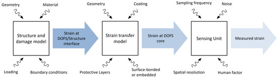
Figure 1.
Flowchart of the proposed MAPOD approach.
First, the model of the structure and damage propagation is required. This model aims to reconstruct the strain at the DOFS/structure interface. One can leverage an existing analytical model based on physics; however, finite element analysis (FEA) might be required for complex geometries. Finally, if the structure or damage propagation is too complex for modeling, one can rely on data-driven models based on experimental data. Regardless of the approach used for modeling the structure, the MAPOD framework requires the user to define a spatial domain vector , representing the extent of the segment of DOFS used for monitoring (see Equation (1)).
The spatial domain is discretized with a user-defined spatial resolution , which must be sufficient to resolve the smallest geometrical feature.
Second, the discrepancy between the strain at the DOFS/structure interface and the DOFS core should not be neglected. This discrepancy can be considered by introducing strain transfer models [34].
Third, the type of interrogation unit affects the final measured strain and must be considered. Within the key variables, particular attention should be given to the human factor, which is often neglected but is of paramount importance. The interrogator resolution can be determinant in certain conditions as well as the signal-to-noise ratio (SNR).
2.2. Strain Transfer
The strain transfer mechanism plays a crucial role in measurement accuracy. Regardless of the working principle, optical fiber sensors measure the deformation of their core, not the deformation of the structure underneath or around it. Therefore, the strain profile at the optical fiber core is a distorted version of the original strain profile present in the structure to be monitored.
The general solution to the strain transfer problem considering a uniform strain field is given by Equation (2) [34,38,39,40,41]:
where is the strain vector of the optical fiber core, the symbol is the input strain vector of the structure, and () is the shear lag parameter, condensing the mechanical and geometrical properties of the system.
Equation (2) is a second-order linear non-homogeneous differential equation with constant coefficients, whose solution is given by Equation (3):
The integration constants and can be determined by applying the corresponding boundary conditions. It is possible to simulate the optical fiber response to a step input of intensity , by imposing the following boundary conditions:
It follows that the integration constants are
Therefore, the step response of the system is given by Equation (6):
It is convenient to define a characteristic space constant , defined as
In this way, Equation (6) can be rewritten as
Equation (8) resembles the step response of a first-order system where the space variable x substitutes the time variable , and the time constant, usually denoted with , is substituted with the characteristic space constant , representing the length required to reach approximately 63% of the strain present in the structure.
Therefore, it is possible to define the positive side () of the system transfer function as
Exploiting the symmetry that should have the transfer function (strain can also propagate backward), it is possible to extend the system transfer function to negative values, which, after normalization, leads to Equation (10):
This result represents the system response to a unit impulse and coincides with the mechanical transfer function proposed by Billon et al., who modeled the strain profile response induced by a surface crack [42]. At this point, it is possible to compute the strain field in the DOFS core, resulting from an arbitrary strain field in the structure , using Equation (11):
Moreover, the characteristic space constant is assumed to vary across the different specimens to take into account the inherent variability associated with the limited repeatability of the bonding process and the possible non-homogeneity of the DOFS coating. Therefore, the characteristic space constant of the ith specimen is sampled from a normal distribution with a mean and a standard deviation:
In a previous study, Falcetelli et al. developed a methodology to compute [34]. This strain transfer model, similar to analogous models available in the literature, requires accurate knowledge of the geometrical and mechanical properties of the optical fiber, the adhesive, and the host structure. However, in most cases, these properties are not available with the required degree of accuracy. Therefore, a more practical approach would be to assess the value of by performing a tensile test with the DOFS bonded in the specimen surface and fitting the chosen analytical model.
Then, by repeating the procedure several times using different specimens, one can improve the accuracy of and assess , thus incorporating the variability associated with the bonding process in the model. It is also interesting to notice that in this MAPOD model, the shear lag constant is considered constant within the specimen, i.e., does not change along the fiber axis but only between different specimens. This assumption holds in cases where the bonding or the embedding is homogeneous without particular geometrical variations along the fiber path. If the fiber is bonded along a longer path, it is reasonable to assume that changes in can also occur within the same specimen. Nevertheless, in this MAPOD study, it is hypothesized that does not change along the fiber length for simplicity.
2.3. Interrogator Resolution
The interrogator resolution is another cause of distortion for the strain profile. In this MAPOD approach, its effect is considered by convolving a rectangular function (Equation (13)) with the DOFS strain profile:
where the symbol denotes a rectangular function having a unitary area and width equal to the interrogator resolution . Hence, the theoretical measured strain profile, , is given by Equation (14):
In Equation (14), the superscript highlights that the measurement is only theoretical, i.e., performed without noise.
2.4. Human Factors
2.4.1. Hot-Touch Error
The first step in DOFS experiments is to locate a certain spatial coordinate in the optical fiber. Indeed, one must correlate the spatial frame of reference in the interrogator software with specific physical points in the DOFS. This is usually done by applying the so-called hot touch, a concentrated heat source, and reading the coordinate of the induced peak in the strain profile in the software. Ideally, the heat source should be infinitely narrow, but in reality, it is not, thus introducing an error in the coordinate locations along the fiber.
In this preliminary stage of the MAPOD framework, this uncertainty source is incorporated into the model using Equation (15) by shifting the vector for each specimen by a quantity , leading to a new translated spatial domain vector ():
where is sampled from a normal distribution with a zero mean and a user-defined standard deviation (), and is a vector of length of ones (Equation (16)):
2.4.2. Bonding Error
The bonding error is the second type of human factor uncertainty source capable of affecting the system response. It is crucial to identify the start and the end of the bonded region in the DOFS. Here, an additional uncertainty source can be present, even assuming a perfect hot-touch procedure is accomplished. Indeed, bonding is never perfect, and the glue can infiltrate underneath the DOFS and thus extend the bonded region by a few millimeters. Moreover, this adhesive leakage, being an undesired effect, is often irregular, leading to unpredictable strain profiles in the transient region on the onset of bonding. Therefore, this uncertainty source must be incorporated into the model and strictly relates to the researcher’s expertise and the available equipment.
In the bonded region, the strain transfer is governed by the equations described in Section 2.2. On the other hand, the strain transfer is posed to zero in the regions outside the bonded area. The bonding error is simply taken into account by increasing or decreasing the bonded region size. In this MAPOD framework, the distance between the onset of the bonded region and the initial crack tip is defined by the parameter as follows:
where and are the mean and random components of . Specifically, is sampled from a normal probability distribution with a zero mean and a bonding error standard deviation.
2.5. Environmental Noise
Noise is modeled by constructing a strain noise vector , defined as
The ith element is defined as
where denotes a normal distribution with a zero mean and a standard deviation equal to . One can assess by performing a series of repeated measurements with no load applied to the specimen.
Finally, the real measured strain , which also takes into account the effect of noise, is obtained by simply superimposing the strain noise vector (Z) to the theoretically measured strain profile , as outlined in Equation (21):
3. The DCB Case Study
Delamination is one of the most common and dangerous damage mechanisms in composite structures, and DCBs are representative structures of many different components. Thanks to well-defined standards describing the experimental procedure [43], DCBs are relatively easy to manufacture and test, which is crucial to validate the MAPOD model.
3.1. Experimental Setup
The DCB specimens are manufactured according to the ASTM D5528 standard [43] employing AS4 HexPly 8552® unidirectional carbon prepreg [44]. The DOFS used in the study is a single-core optical fiber with ORMOCER® coating [45]. The fiber is bonded on the surface of the specimen using a cyanoacrylate adhesive (ThreeBond 1742® [46]). In the experiment, three DOFS segments are bonded on the top surface to augment the available data collected in the static test.
Figure 2 illustrates the specimen geometry and the relative DOFS installation layout used for the DCB static test.
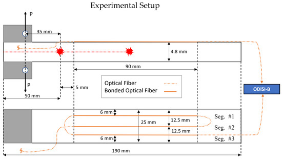
Figure 2.
DCB scheme and DOFS layout for the static test (adapted from Falcetelli et al. [17]).
The fibers are interrogated with the ODiSI-B [47] measuring system, which uses swept-wavelength coherent interferometry to estimate Rayleigh backscattering [48,49,50]. The spatial resolution and the sampling frequency of the sensing unit are 0.65 mm and 23.8 Hz, respectively. The DCB specimen is fixed on a Zwick—20 kN tensile test machine, and the load is applied with a displacement rate of 1 mm/min. The true crack length is estimated by exploiting its linear relationship with the cube root of the compliance value. The linear model is fitted by observing the delamination size from a 9-megapixel camera placed in front of the tensile test machine at different compliance values. Further details on the experimental setup can be found in Falcetelli et al. [17].
3.2. DCB Parametric Model
This section introduces a simplified DCB model, based on the experimental data derived in the previous section, to validate the proposed MAPOD methodology. Figure 3 describes the specimen geometry and the relative DOFS position.
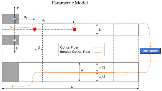
Figure 3.
DCB scheme and DOFS layout of the proposed parametric model.
In the parametric model, it is not necessary to consider three fiber segments on the DCB surface since the only limitation in the amount of synthetically generated data is the computational cost involved in the simulation. Therefore, it was decided to consider only a single DOFS segment bonded in the longitudinal direction at the center of the specimen to simplify the model.
The objective in this phase is to derive the strain distribution on the surface of the DCB specimen, , which is then fed into the strain transfer model.
Considering the two DCB arms as cantilever beams and referring to the Euler–Bernoulli theory, it is possible to compute the bending moment about the z-axis (perpendicular to the paper and pointing outward in Figure 3) as a function of the distance from the crack tip [51]:
Equation (22) holds for since must be null after the crack tip at , where denotes the crack length.
The applied load, , decreases with the delamination length according to a function that can be determined experimentally or through FEM simulations [52]. In this case, was determined by a third-degree polynomial regression (Equation (23)) using the experimental static test data of the DOFS with ORMOCER® coating [17].
The random component accounts for the impossibility of reproducing the exact loading condition across different specimens:
where represents the standard deviation of the normal distribution with a mean equal to zero. Its value can be assessed from the analysis of previous experimental activity or based on the expected operational loading conditions for a given application.
Applying Navier’s formula (Equation (25)) to the upper arm of the DCB shown in Figure 3, one can find the stress distribution along the x-axis, :
where is the spatial coordinate along the thickness direction, and denotes the moment of inertia about the z-axis (perpendicular to the paper pointing outward in Figure 3). The moment of inertia for a rectangular cross-section with a width and height equal to and , respectively, can be computed as follows:
Moreover, the specimen width and thickness could vary across the different specimens due to the variability in the manufacturing process. The variability can be estimated by measuring the specimens under test with a caliper. In this case study, the width and thickness variabilities were considered negligible compared to other uncertainty sources.
Finally, the strain on the DCB surface, , can be obtained by dividing the stress distribution along the x-axis, , by the flexural modulus :
The flexural modulus was computed using the following Equation (28), referring to the ASTM D5528 standard [43]:
where denotes the compliance and is defined as the ratio between the load point deflection, , and the applied load, . On the other hand, is a crack length correction used to account for the possible rotation at the crack tip. Its value corresponds to the abscissa where the least squares regression of the cube root of compliance, , against the delamination length, , is equal to zero.
Then, the expected strain distribution along the x-axis at the specimen surface is obtained by substituting the value of , obtained posing in Equation (25) into Equation (27):
3.3. Delamination Modeling from a MAPOD Perspective
The proposed MAPOD approach simulates delamination growth in a DCB specimen of length , for a user-defined number of cracks, , starting from a user-defined initial crack length, , to a user-defined final crack length, . It is assumed that every crack length measurement is taken after a certain delamination length increment, . The true crack length, , is usually visually estimated, thus introducing uncertainty in the model. Therefore, it is further assumed that is composed of a mean constant value, , and a random error, :
where follows a normal probability distribution with a zero mean and a standard deviation :
The value is challenging to assess and depends on many factors, such as the loading type, the geometry, and the material properties. Therefore, the best option is to evaluate using data from a pilot study experiment.
On the other hand, can be computed as
Then, the model generates a vector of crack lengths, , which is defined in Equation (33):
where and are the mean and random vectors of crack lengths defined in Equations (34) and (35), respectively:
In this case, the spatial domain, , is discretized with a user-defined spatial resolution, , which must be sufficiently smaller than the average delamination increment, and thus it must be that . This implies that the spatial domain vector, x, defined in Equation (1), has elements, with .
4. Results
4.1. Model Validation
Table 1 shows the parameter configuration for the following demonstrative example, classifying the sources of uncertainty into within- and between-specimen variability (if the parameters are just model settings, they belong to neither of the two classes).

Table 1.
MAPOD parameter setting.
Figure 4 shows the model outputs for the strain profile at the DOFS/DCB interface (top), the DOFS core (middle), and the interrogator-measured strain (bottom). Every line symbolizes the strain profile given at a specific crack length value, highlighted by the color bar on the right-hand side. The vertical dashed line shows the onset of the bonded region of the DOFS. It is possible to notice that since the DOFS is bonded 5 mm apart from the initial crack length, the fiber is not sensitive to damage at the initial phase of delamination growth. Once delamination reaches the bonded region and eventually grows underneath the DOFS, the measured strain profiles bend downward. The black star-shaped markers in the bottom subplot of Figure 4 indicate the absolute minimum of the strain profile, where the crack tip is expected to be located [32,53].
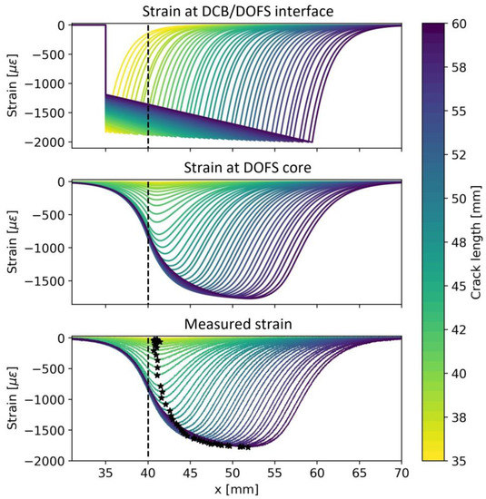
Figure 4.
Simulation of strain profiles for different delamination lengths at the DCB surface (top), DOFS core (middle), and interrogator (bottom). The black star-shaped markers indicate the absolute minimum of the strain profile, where the crack tip is expected to be located.
In Figure 5, experimental data (left) are compared with the results predicted by the model (right). From a qualitative perspective, it is possible to notice that experimental data show a higher degree of variability along the DOFS axis. Several factors can cause the difference. First, the proposed DCB model is still a simplified version of the real DCB, which would require a higher level of modeling to achieve more accurate results. For example, the model does not consider the possibility of having a curved crack front, which is common in DCB specimens. One might also note that the process zone can affect the strain at the specimen surface, but all these considerations are outside the scope of this paper. Second, the mechanical transfer function, , used to predict the strain transfer does not vary with the coordinate. This assumption neglects the presence of occasional defects in the bonding. These fluctuations in might also be due to the intrinsic flaws present in the coating of the fiber.
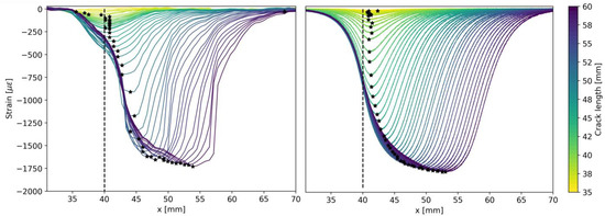
Figure 5.
Measured strain profiles in DCB quasi-static test [17]: experimental data (left) and MAPOD predicted result (right). The black star-shaped markers indicate the absolute minimum of the strain profile, where the crack tip is expected to be located.
The model validation continues through Section 4.1.1, where the experimental POD curve is compared with the MAPOD curve.
4.1.1. Length at Detection Method and MAPOD Curve
As stated in the introduction section, the derivation of POD or MAPOD curves in SHM is substantially different from the NDE case due to the spatial and temporal correlation typical of SHM systems.
In NDE, every specimen returns a single point in the traditional or equivalent model: , , , and . In other words, every point corresponds to a measurement taken from a certain specimen, guaranteeing statistical independence. On the other hand, in SHM, every specimen returns a series of spatial- and time-correlated data since the permanently installed sensor continuously monitors the damage evolution.
Therefore, the application of the method (or the hit/miss method in the case of binary data), as initially conceived in the MIL-HKBK-1823A [12] for NDE applications, would lead to inconsistent results. Among the available statistical methods to handle SHM data, the LaD offers an intuitive and easy-to-implement approach. The alternative REM-based methodology has the advantage of using data more efficiently but at the expense of increasing the complexity of the algorithm and the computational burden [15]. Therefore, in this preliminary development of the MAPOD framework for DOFSs, the LaD is selected as the most appropriate approach.
In the LaD method, a certain damage index (DI) is plotted against a certain damage-related feature, in this case, the delamination length. However, differently from the traditional approach, the procedure is repeated for every specimen, leading to a number of regression lines equal to the number of specimens considered in the analysis.
The LaD method can handle spatial and temporal correlated data because it considers only the measurements in correspondence with the first detection, which is the intersection of every line with the user-defined threshold. Therefore, the threshold line contains a population of crack/delamination lengths at detection which is usually assumed to follow a normal or log-normal probability distribution. Therefore, assuming that the population is normally distributed, it is possible to compute the POD curve as follows:
where denotes the standard normal distribution cumulative distribution function, and and are the sample mean and standard deviation, respectively.
The lower confidence bound can be computed with the one-sided tolerance interval (OSTI) approach [54]:
where and are the tolerance interval and factor, respectively. The tolerance factor depends on the sample size (in this case, the number of specimens, ), the confidence level , and the detection level . A standard procedure to compute its value exploits the properties of the non-central t-distribution [15].
The LaD method requires defining a proper DI. The DI definition depends on the sensor technology and the type of damage to be monitored. For example, in certain cases, to obtain a DI, one can leverage multi-sensor data fusion [55,56] or more complex strategies based on deep learning [57]. In this study, involving delamination monitoring using DOFSs, it is logical to consider some damage-induced strain feature as DI. The most straightforward choice is to define the DI related to a certain crack length as the strain value recorded at the absolute minimum of each strain profile. Referring to Figure 5, this translates into considering the strain values in correspondence with the black star-shaped markers as a DI.
Then, one can take the absolute value and obtain a monotonically increasing DI as described by Equation (38):
For validation purposes, the same threshold value was used as in the previous experimental study [17] of . Applying the LaD method using the DI defined in Equation (38) returns the plot shown in Figure 6.
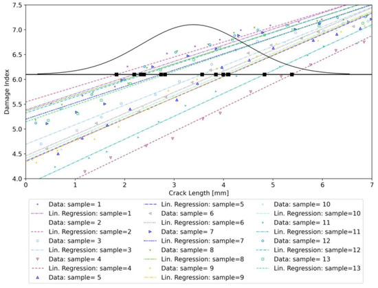
Figure 6.
Model-Assisted LaD method applied to synthetic DOFS data for crack detection.
Every regression line is associated with a different specimen and has its own slope and intercept, reflecting between-specimen variability. At the same time, data belonging to the same specimen are scattered around the mean value represented by the regression line, showing within-specimen variability (see Table 1).
Assuming that the crack lengths at detection are normally distributed, it is possible to obtain the corresponding POD curve (see Figure 7) by computing the cumulative function of the LaD distribution. The distance of the lower 95% confidence bound (blue dashed line) from the POD curve (solid black line) reflects system uncertainty. High uncertainty values in the model parameters will result in a lower 95% confidence bound far away from the original POD curve.
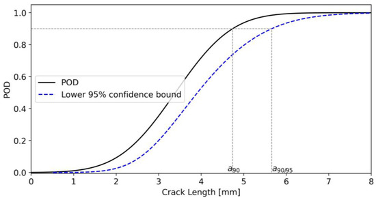
Figure 7.
POD and its lower 95% confidence bound for simulated data.
One can verify the normality assumption of the LaD method with the so-called Anderson–Darling test (Figure 8). The null hypothesis assumes that the data are normally distributed and should be rejected if, for a given significance level , the critical value is lower than the Anderson–Darling statistics (A2). With and , the critical value equals 0.679. The A2 statistics for the simulated LaD data plotted is 0.329. Thus, according to the normality test, should not be rejected and the crack lengths at detection can be considered normally distributed.
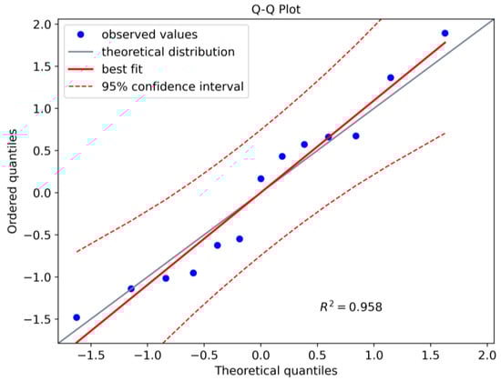
Figure 8.
Normality Test for the LaD method.
Finally, Table 2 compares the experimental and MAPOD values for (the crack length value having a 90% probability of being detected) and (the crack length value having a 90% probability of being detected with 95% confidence). The relative error for is , whereas the relative error for is , demonstrating the accuracy of the proposed model.
Table 2.
Comparison of experimental and simulated and .
4.2. Sensitivity Analysis
In this section, the objective is to perform a preliminary qualitative analysis of the effect of the most important variables on the and generated through the MAPOD curves. The threshold definition is crucial in this analysis and can significantly affect the result. The threshold value must guarantee a constant probability of false alarm (PFA). In the literature, no standard methodology defines the threshold for the LaD method. Here, the threshold was defined according to Equation (39):
where, represents the vector containing the measured strain values at the onset of the bonded region for each specimen. Therefore, is chosen by adding three noise standard deviations to the highest measured strain values between the tested samples at the onset of the bonded region. This definition is noise-dependent, which is coherent with maintaining a constant PFA, and prevents the possibility of obtaining negative crack lengths at detection.
Table 3 shows the parameter settings used in the sensitivity analysis. The data structure symbolizes that the parameter is linearly swept from an initial value (first field) to a final value (second field) on a logarithmic scale with a certain number of elements (third field). For example, means that is linearly swept on a logarithmic scale from 0.001 mm to 20 mm considering 100 elements.
Table 3.
Parameter setting for the sensitivity analysis.
4.2.1. Noise Effect (Case 1)
Figure 9 illustrates the effect of measurement noise on the detection performance. The results show that the effect of noise is observable only for standard deviation values higher than . This result might seem counterintuitive since is a relatively high value for common applications, and one would expect a degradation of the performance starting from lower values of . However, to comprehend the result, one must distinguish between detection and localization performance and how the DI and the threshold value are defined. Indeed, in terms of localization, the performance is compromised even at lower values, because the minimum peaks in the strain profile would be scattered along the fiber length and mainly attributed to noise. However, the system is much more robust in terms of crack detection. Indeed, the DI (see Equation (38)) considers only the strain value in the minimum of a given strain profile, not its location. This definition allows the model to find a relation between the and even in particularly noisy conditions. The limit of depends on the specific application of and especially on the damage-induced strain. In this DCB case study, below , the SNR is still high enough to make a detection. However, if the damage-induced strain is low, the effect of noise would be much more disruptive even at lower values. It is important to highlight that the threshold definition is of paramount importance. According to Equation (39), the threshold increases with , and this guarantees a constant PFA. With a fixed threshold value, we would witness the paradoxical and fictitious improvement of the detection performance caused by a corresponding increase in the PFA.
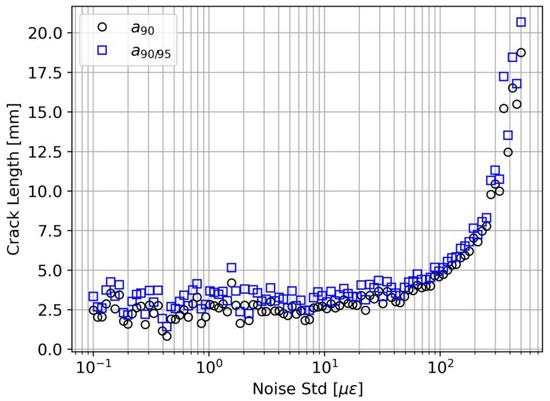
Figure 9.
Noise effect on and .
4.2.2. Strain Transfer Effect (Case 2)
The shear lag constant effect on the detection capabilities is highlighted in Figure 10. When , and show a steady value of around 4 mm. Then, for , it is possible to observe a sudden increase in and . This means that stiffer DOFSs, characterized by low values, have better detection performance, but the benefit is negligible for values lower than 1 mm.
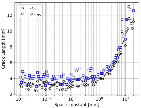
Figure 10.
Space constant effect on and .
This analysis can also be used to implement a degradation model of the DOFS coupling with the structure. Indeed, different values of can correspond to different adhesives but also subsequent moments in time of the same adhesive undergoing aging.
4.2.3. Interrogator Resolution Effect (Case 3)
Figure 11 is composed of three subplots, representing the effect of the interrogator resolution Δx at three different noise levels: , , and . In principle, an ideal interrogator with an infinite spatial resolution () should provide the best performance. Figure 11 confirms this belief but only to a certain extent, depending on the noise level. At low noise levels (), the resolution effect on and is negligible. Indeed, even if a poor resolution flattens the measured strain profile, the SNR is still high enough to ensure comparable detection performance. Once again, similarly to what emerged in Section 4.2.1, one must distinguish detection performance from localization performance. At a higher noise level (), the effect of the interrogator resolution is observable. Finally, as the noise level increases even further (), the critical SNR is reached at even lower values of . This kind of simulation can be beneficial to the engineer in selecting the right interrogator in the preliminary design phase of the SHM system. Indeed, considering all the available information about the other model parameters, the SHM system equipped with such an interrogator should satisfy specific requirements for and .
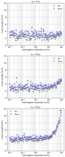
Figure 11.
Interrogator resolution effect on and , at (top), (middle), and (bottom).
4.2.4. Hot-Touch Error Effect (Case 4)
The hot-touch standard deviation reflects one of the human factor effects on the detection performance. It is important to point out that in a noisy environment, performing a satisfactory hot-touch procedure is extremely difficult. Hot-touch standard deviation values greater than 1 mm in real operational conditions are relatively common. However, Figure 12 suggests that can deeply change the detection performance of the system starting from . As pointed out for the previous cases, this value can change depending on the other model parameters, but it is fundamental to notice how a procedure that is often considered of minor importance can have a considerable impact on and .
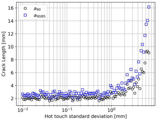
Figure 12.
Interrogator resolution effect on and .
4.2.5. Bonding Error Effect (Case 5)
The bonding error is a second possible human factor issue that can potentially affect the performance of the system. The semi-logarithmic plot illustrated in Figure 13 shows that a lack of repeatability in the bonding procedure could lead to a detrimental effect. It is important to notice that this deterioration of the detection performance can start already at relatively low values of , even lower than 1 mm. The result is somewhat expected since an error in the starting point of the bonded region would inevitably anticipate or delay the strain transfer process. As a consequence, data will be more scattered, the threshold will increase, and the result POD curve will produce higher and values.
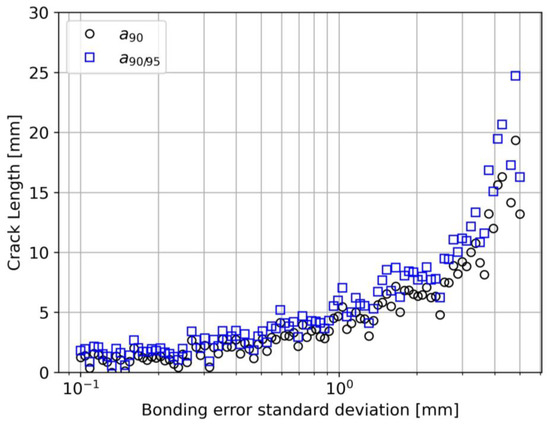
Figure 13.
Bonding error standard deviation effect on and .
5. Discussion
Upscaling of the MAPOD Methodology to a Real Aerospace Structure
From a practical perspective, assessing the upscaling capabilities of the presented MAPOD framework is crucial. In other words, it is essential to understand whether it is possible to transpose the MAPOD curves to a higher structural component in a building block approach.
Referring to the flowchart of the proposed MAPOD approach (see Figure 1), one can notice that the interrogator block receives as input the results of the strain transfer block, and the strain transfer block receives as inputs the outputs of the structure/damage block. Therefore, upscaling the presented MAPOD framework to a more complex and representative structural item would impact only the first block, which is highly desirable.
Therefore, applying the presented MAPOD framework to a more realistic case implies substituting the first block (DCB model described in Section 3) with another block representing the new structure.
For example, debonding and delamination can occur in stiffened panels at the skin–stringer interface or between adjacent layers having different fiber orientations [58]. In this case, one could directly model the stiffened composite panel using finite element analysis (FEA) or by whatever model that can return as outputs the strain values at the DOFS/ structure interface in the presence of damage.
Several studies have investigated debonding and delamination in stiffened composite panels for aerospace applications in a damage tolerance scenario with DOFSs [59,60] and FBGs [61], considering damage sizes in the 40–80 mm range. In this study, it is shown that in a DCB specimen, it is possible to achieve of 5.66 mm (see Table 2). However, a direct transposition of this result to a full-scale composite panel would be misleading. Indeed, in a skin–stringer debonding scenario, delamination can occur at different mode-mixity [62,63], and the DOFS sensitivity can differ for different opening modes.
A solution would be developing MAPOD curves at a specimen level for different opening modes and opening mode-mixity. Then, using a building block approach [64], one could transpose the results to a higher-level component, selecting the MAPOD curve obtained in the scenario that better approximates the expected strain field near the damaged location.
The authors believe that upscaling POD and MAPOD curves is crucial for concrete and sustainable deployment of SHM in primary composite structures and certainly deserves further investigation.
6. Conclusions
This study focuses on the development of a MAPOD framework for DOFSs. This framework has never been established for DOFSs, only for a few SHM technologies such as GLW, bulk-wave ultrasonic sensors, and FBGs. From a methodological perspective, the modeling was divided into three blocks: the structure and damage model, the strain transfer model, and the sensing unit model. Each block receives as input several uncertainty sources, which were analyzed and modeled. The model was validated with previously collected data on an equivalent case study, showing comparable and values. The results of the sensitivity analysis highlight the main variables affecting POD curves and, specifically, and . These variables are the noise, the strain transfer space constant, the interrogator resolution, and the human factors (hot-touch and bonding errors).
Table 4 summarizes the sensitivity analysis results. For each case, it is shown the value obtained in correspondence with equal to 10 mm and in correspondence with a 10% raise () of with respect to its initial steady state value. Assuming that 10 mm is the maximum allowed delamination size for a given application, the first value can be considered the critical parameter threshold that should not be exceeded. On the other hand, the second value symbolizes the threshold below which the parameter does not affect the MAPOD curve. In other words, any effort to reduce its value does not produce any improvement in terms of .
Table 4.
Summary of the sensitivity analysis results.
The impact of noise on damage detection is negligible until the SNR falls below a critical value. The MAPOD approach for the selected case study showed that the system is robust against noise standard deviation values below approximately . The strain transfer analysis highlighted that and significantly increase for space constant values higher than approximately 1 mm. This result is the first of its kind since the strain transfer problem has never been analyzed in an SHM damage detection probabilistic framework. The effect of the interrogator resolution was negligible for low values of noise , but its effect has been observed for higher noise values . The human factors, namely the hot-touch and bonding errors, were also analyzed. These kinds of uncertainty sources have never been analyzed before this research and were revealed to be key variables with a significant impact on and .
This research has unfolded only some aspects of SHM systems based on DOFSs applied to composite structures undergoing mode I static loading conditions. The model should be further refined to model even more uncertainty sources, such as a variable strain transfer function along the optical fiber length, or to simulate other loading conditions (such as fatigue) or crack opening modes (mode II and mode III).
The proposed approach could be used for modeling changing EOCs and simulating their effect on POD curves. For instance, increasing the strain transfer constant in time would reproduce a degradation of the strain transfer properties expected with the aging of the adhesive or the optical fiber coating.
This MAPOD framework appears promising to study not only detection but also localization and sizing problems. The extension of this approach to the subsequent steps of the SHM paradigm would lead to the development of the model-assisted probability of localization and sizing (MAPOL and MAPOS). The application of the presented approach to MAPOL and MAPOS will be the subject of future studies.
Author Contributions
Conceptualization, F.F. and N.Y.; methodology, F.F. and N.Y.; software, F.F.; validation, F.F. and N.Y.; formal analysis, F.F. and N.Y.; investigation, F.F.; resources, D.Z., G.B. and F.B.; data curation, F.F.; writing—original draft preparation, F.F. and N.Y.; writing—review and editing, L.R., R.D.S. and D.Z.; visualization, F.F., L.R. and N.Y.; supervision, R.D.S. and D.Z.; project administration, R.D.S. and D.Z.; funding acquisition, G.B. and F.B. All authors have read and agreed to the published version of the manuscript.
Funding
This activity has received funding from the European Union through Horizon 2020, the Framework Programme for Research and Innovation, under project SLAM DAST, Grant Agreement No. 971149.
Institutional Review Board Statement
Not applicable.
Informed Consent Statement
Not applicable.
Data Availability Statement
Not applicable.
Conflicts of Interest
The authors declare no conflict of interest.
References
- Guo, H.; Xiao, G.; Mrad, N.; Yao, J. Fiber Optic Sensors for Structural Health Monitoring of Air Platforms. Sensors 2011, 11, 3687–3705. [Google Scholar] [CrossRef]
- Glišić, B.; Inaudi, D. Fibre Optic Methods for Structural Health Monitoring; John Wiley & Sons: Chichester, UK; Hoboken, NJ, USA, 2007; ISBN 978-0-470-06142-8. [Google Scholar]
- Güemes, A.; Fernández-López, A.; Díaz-Maroto, P.; Lozano, A.; Sierra-Perez, J. Structural Health Monitoring in Composite Structures by Fiber-Optic Sensors. Sensors 2018, 18, 1094. [Google Scholar] [CrossRef]
- Rufai, O.; Chandarana, N.; Gautam, M.; Potluri, P.; Gresil, M. Cure Monitoring and Structural Health Monitoring of Composites Using Micro-Braided Distributed Optical Fibre. Compos. Struct. 2020, 254, 112861. [Google Scholar] [CrossRef]
- Falcetelli, F.; Di Sante, R.; Troiani, E. Strategies for Embedding Optical Fiber Sensors in Additive Manufacturing Structures. In European Workshop on Structural Health Monitoring; Rizzo, P., Milazzo, A., Eds.; Lecture Notes in Civil Engineering; Springer International Publishing: Cham, Switzerland, 2021; Volume 128, pp. 362–371. ISBN 978-3-030-64908-1. [Google Scholar]
- Kashyap, R. Fiber Bragg Gratings, 2nd ed.; Academic Press: Burlington, MA, USA, 2010; ISBN 978-0-12-372579-0. [Google Scholar]
- Cusano, A.; Cutolo, A.; Albert, J. (Eds.) Fiber Bragg Grating Sensors: Recent Advancements, Industrial Applications and Market Exploitation; Bentham Science Publishers: Sharjah, United Arab Emirates, 2012; ISBN 978-1-60805-084-0. [Google Scholar]
- Lu, P.; Lalam, N.; Badar, M.; Liu, B.; Chorpening, B.T.; Buric, M.P.; Ohodnicki, P.R. Distributed Optical Fiber Sensing: Review and Perspective. Appl. Phys. Rev. 2019, 6, 041302. [Google Scholar] [CrossRef]
- Palmieri, L.; Schenato, L.; Santagiustina, M.; Galtarossa, A. Rayleigh-Based Distributed Optical Fiber Sensing. Sensors 2022, 22, 6811. [Google Scholar] [CrossRef]
- Cawley, P. Structural Health Monitoring: Closing the Gap between Research and Industrial Deployment. Struct. Health Monit. 2018, 17, 1225–1244. [Google Scholar] [CrossRef]
- Falcetelli, F.; Yue, N.; Di Sante, R.; Zarouchas, D. Probability of Detection, Localization, and Sizing: The Evolution of Reliability Metrics in Structural Health Monitoring. Struct. Health Monit. 2022, 21, 2990–3017. [Google Scholar] [CrossRef]
- Department of Defense Handbook: Nondestructive Evaluation System Reliability Assessment; Department of Defense: Washington, DC, USA, 2009.
- Schubert Kabban, C.M.; Greenwell, B.M.; DeSimio, M.P.; Derriso, M.M. The Probability of Detection for Structural Health Monitoring Systems: Repeated Measures Data. Struct. Health Monit. 2015, 14, 252–264. [Google Scholar] [CrossRef]
- Janapati, V.; Kopsaftopoulos, F.; Li, F.; Lee, S.J.; Chang, F.-K. Damage Detection Sensitivity Characterization of Acousto-Ultrasound-Based Structural Health Monitoring Techniques. Struct. Health Monit. 2016, 15, 143–161. [Google Scholar] [CrossRef]
- Meeker, W.Q.; Roach, D.; Kessler, S.S. Statistical Methods for Probability of Detection in Structural Health Monitoring. In Proceedings of the Structural Health Monitoring 2019, Stanford, CA, USA, 10–12 September 2019; DEStech Publications, Inc.: Stanford, CA, USA. [Google Scholar]
- Kessler, S.S.; Dunn, C.T.; Swindell, P.; Meeker, W. Detection Sensitivity Analysis for a Potential Drop (PD) Structural Health Monitoring (SHM) System. In Proceedings of the 12th International Workshop on Structural Health Monitoring, Stanford, CA, USA, 10–12 September 2019; DEStech Publications, Inc.: Stanford, CA, USA. [Google Scholar]
- Falcetelli, F.; Cristiani, D.; Yue, N.; Sbarufatti, C.; Troiani, E.; Di Sante, R.; Zarouchas, D. Qualification of Distributed Optical Fiber Sensors Using Probability of Detection Curves for Delamination in Composite Laminates. Struct. Health Monit. 2022, 147592172211411. [Google Scholar] [CrossRef]
- Thompson, R.B.; Thompson, D.O.; Chimenti, D.E. A Unified Approach to the Model-Assisted Determination of Probability of Detection. In Proceedings of the AIP Conference Proceedings, Golden, CO, USA, 22–27 July 2007; AIP: Golden, CO, USA, 2008; Volume 975, pp. 1685–1692. [Google Scholar]
- Aldrin, J.C.; Knopp, J.S.; Lindgren, E.A.; Jata, K.V.; Thompson, D.O.; Chimenti, D.E. Model-Assisted Probability of Detection Evaluation for Eddy Current Inspection of Fastener Sites. In Proceedings of the AIP Conference Proceedings, Chicago, IL, USA, 20–25 July 2008; AIP: Chicago, IL, USA, 2009; pp. 1784–1791. [Google Scholar]
- Thompson, R.B.; Brasche, L.J.; Forsyth, D.; Lindgren, E.A.; Swindell, P.; Winfree, W. Recent Advances in Model-Assisted Probability of Detection; NDT.net: Berlin, Germany, 2009. [Google Scholar]
- Foucher, F.; Fernandez, R.; Leberre, S.; Calmon, P. New Tools in CIVA for Model Assisted Probability of Detection (MAPOD) to Support NDE Reliability Studies; ASNT: Bridgeton, MO, USA, 2018; p. 12. [Google Scholar]
- Foucher, M.F.; Lonne, S.; Toullelan, G.; Mahaut, S.; Chatillon, S. An Overview of Validation Campaigns of the CIVA Simulation Software; NDT.net: Gothenburg, Sweden, 2018; p. 9. [Google Scholar]
- Aldrin, J.C.; Medina, E.A.; Lindgren, E.A.; Buynak, C.F.; Knopp, J.S. Protocol for Reliability Assessment of Structural Health Monitoring Systems Incorporating Model-Assisted Probability of Detection (MAPOD) Approach. In Proceedings of the 8th International Workshop on Structural Health Monitoring, Stanford, CA, USA, 13 September 2011; pp. 2452–2459. [Google Scholar]
- Tschoke, K.; Mueller, I.; Memmolo, V.; Moix-Bonet, M.; Moll, J.; Lugovtsova, Y.; Golub, M.; Venkat, R.S.; Schubert, L. Feasibility of Model-Assisted Probability of Detection Principles for Structural Health Monitoring Systems Based on Guided Waves for Fibre-Reinforced Composites. IEEE Trans. Ultrason. Ferroelect. Freq. Contr. 2021, 68, 3156–3173. [Google Scholar] [CrossRef] [PubMed]
- Moriot, J.; Quaegebeur, N.; Le Duff, A.; Masson, P. A Model-Based Approach for Statistical Assessment of Detection and Localization Performance of Guided Wave–Based Imaging Techniques. Struct. Health Monit. 2018, 17, 1460–1472. [Google Scholar] [CrossRef]
- Leung, M.S.H.; Corcoran, J. Evaluating the Probability of Detection Capability of Permanently Installed Sensors Using a Structural Integrity Informed Approach. J. Nondestruct. Eval. 2021, 40, 82. [Google Scholar] [CrossRef]
- Falcetelli, F.; Venturini, N.; Romero, M.B.; Martinez, M.J.; Pant, S.; Troiani, E. Broadband Signal Reconstruction for SHM: An Experimental and Numerical Time Reversal Methodology. J. Intell. Mater. Syst. Struct. 2021, 32, 1043–1058. [Google Scholar] [CrossRef]
- Gagar, D.; Irving, P.E.; Jennions, I.K.; Foote, P.; Read, I.; McFeat, J. Development of Probability of Detection Data for Structural Health Monitoring Damage Detection Techniques Based on Acoustic Emission. In Proceedings of the 8th International Workshop on Structural Heath Monitoring, Stanford, CA, USA, 13 September 2011; pp. 1391–1398. [Google Scholar]
- Falcetelli, F.; Barroso-Romero, M.; Pant, S.; Troiani, E.; Martinez, M. Modelling of Pencil-Lead Break Acoustic Emission Sources Using the Time Reversal Technique. In Proceedings of the EWSHM 2018, Manchester, UK, 10–13 July 2018; NDT.net: Manchester, UK, 2018. [Google Scholar]
- Sbarufatti, C.; Giglio, M. Performance Qualification of an On-Board Model-Based Diagnostic System for Fatigue Crack Monitoring. J. Am. Helicopter Soc. 2017, 62, 1–10. [Google Scholar] [CrossRef]
- Sbarufatti, C.; Corbetta, M.; San Millan, J.; Frovel, M.; Stefaniuk, M.; Giglio, M. Model-Assisted Performance Qualification of a Distributed SHM System for Fatigue Crack Detection on a Helicopter Tail Boom. In Proceedings of the EWSHM 2016, Bilbao, Spain, 5 July 2016. [Google Scholar]
- Lima, R.A.A.; Migliavacca, F.; Martulli, L.M.; Carboni, M.; Bernasconi, A. Distributed Fibre Optic Monitoring of Mode I Fatigue Crack Propagation in Adhesive Bonded Joints and Comparison with Digital Image Correlation. Theor. Appl. Fract. Mech. 2022, 121, 103501. [Google Scholar] [CrossRef]
- Stutz, S.; Cugnoni, J.; Botsis, J. Studies of Mode I Delamination in Monotonic and Fatigue Loading Using FBG Wavelength Multiplexing and Numerical Analysis. Compos. Sci. Technol. 2011, 71, 443–449. [Google Scholar] [CrossRef]
- Falcetelli, F.; Rossi, L.; Di Sante, R.; Bolognini, G. Strain Transfer in Surface-Bonded Optical Fiber Sensors. Sensors 2020, 20, 3100. [Google Scholar] [CrossRef]
- Ansari, F.; Libo, Y. Mechanics of Bond and Interface Shear Transfer in Optical Fiber Sensors. J. Eng. Mech. 1998, 124, 385–394. [Google Scholar] [CrossRef]
- Yan, M.; Tan, X.; Mahjoubi, S.; Bao, Y. Strain Transfer Effect on Measurements with Distributed Fiber Optic Sensors. Autom. Constr. 2022, 139, 104262. [Google Scholar] [CrossRef]
- Mueller, C.; Bertovic, M.; Pavlovic, M.; Kanzler, D.; Ewert, U.; Pitkänen, J.; Ronneteg, U. Paradigm Shift in the Holistic Evaluation of the Reliability of NDE Systems. Mater. Test. 2013, 55, 261–269. [Google Scholar] [CrossRef]
- Li, H.-N.; Zhou, G.-D.; Ren, L.; Li, D.-S. Strain Transfer Coefficient Analyses for Embedded Fiber Bragg Grating Sensors in Different Host Materials. J. Eng. Mech. 2009, 135, 1343–1353. [Google Scholar] [CrossRef]
- Li, D.-S.; Li, H.; Ren, L.; Song, G. Strain Transferring Analysis of Fiber Bragg Grating Sensors. Opt. Eng. 2006, 45, 024402. [Google Scholar] [CrossRef]
- Her, S.-C.; Huang, C.-Y. Effect of Coating on the Strain Transfer of Optical Fiber Sensors. Sensors 2011, 11, 6926–6941. [Google Scholar] [CrossRef] [PubMed]
- Wang, H.; Xiang, P.; Jiang, L. Strain Transfer Theory of Industrialized Optical Fiber-Based Sensors in Civil Engineering: A Review on Measurement Accuracy, Design and Calibration. Sens. Actuators A Phys. 2019, 285, 414–426. [Google Scholar] [CrossRef]
- Billon, A.; Hénault, J.-M.; Quiertant, M.; Taillade, F.; Khadour, A.; Martin, R.-P.; Benzarti, K. Qualification of a Distributed Optical Fiber Sensor Bonded to the Surface of a Concrete Structure: A Methodology to Obtain Quantitative Strain Measurements. Smart Mater. Struct. 2015, 24, 115001. [Google Scholar] [CrossRef]
- D30 Committee Test Method for Mode I Interlaminar Fracture Toughness of Unidirectional Fiber-Reinforced Polymer Matrix Composites; ASTM International Headquarter: West Conshohocken, PA, USA.
- Hexcel HexPly® 8552 UD Carbon Prepregs. Available online: https://www.hexcel.com/user_area/content_media/raw/HexPly_8552_eu_DataSheet.pdf (accessed on 3 February 2022).
- FBGS Technologies GmbH ORMOCER® Coating. Available online: https://fbgs.com/technology/ormocer-coating/ (accessed on 4 February 2022).
- Product Information—TB1742. Available online: https://threebond-europe.com/products/tb1742/ (accessed on 4 February 2022).
- Optical Distributed Sensor Interrogator Model ODiSI-B: User’s Guide; Luna Innovations Inc.: Roanoke, VA, USA, 2017.
- Gifford, D.K.; Kreger, S.T.; Sang, A.K.; Froggatt, M.E.; Duncan, R.G.; Wolfe, M.S.; Soller, B.J. Swept-Wavelength Interferometric Interrogation of Fiber Rayleigh Scatter for Distributed Sensing Applications. In Proceedings of the Fiber Optic Sensors and Applications V, Boston, MA, USA, 12 October 2007; International Society for Optics and Photonics: Boston, MA, USA, 2007; Volume 6770, p. 67700F. [Google Scholar]
- Soller, B.J.; Wolfe, M.S.; Froggatt, M.E. Polarization Resolved Measurement of Rayleigh Backscatter in Fiber-Optic Components. In Proceedings of the OFC Technical Digest, Anaheim, CA, USA, 6 March 2005; OSA Publishing: Anaheim, CA, USA, 2005. [Google Scholar]
- Kreger, S.T.; Gifford, D.K.; Froggatt, M.E.; Soller, B.J.; Wolfe, M.S. High Resolution Distributed Strain or Temperature Measurements in Single- and Multi-Mode Fiber Using Swept-Wavelength Interferometry. In Proceedings of the Optical Fiber Sensors, Cancún, Mexico, 23–27 October 2006; OSA: Cancún, Mexico, 2006; p. ThE42. [Google Scholar]
- Škec, L.; Alfano, G.; Jelenić, G. Enhanced Simple Beam Theory for Characterising Mode-I Fracture Resistance via a Double Cantilever Beam Test. Compos. Part B Eng. 2019, 167, 250–262. [Google Scholar] [CrossRef]
- Cristiani, D.; Sbarufatti, C.; Giglio, M. Damage Diagnosis and Prognosis in Composite Double Cantilever Beam Coupons by Particle Filtering and Surrogate Modelling. Struct. Health Monit. 2021, 20, 1030–1050. [Google Scholar] [CrossRef]
- Truong, H.T.X.; Martinez, M.J.; Ochoa, O.O.; Lagoudas, D.C. Mode I Fracture Toughness of Hybrid Co-Cured Al-CFRP and NiTi-CFRP Interfaces: An Experimental and Computational Study. Compos. Part A Appl. Sci. Manuf. 2020, 135, 105925. [Google Scholar] [CrossRef]
- Roach, D. Real Time Crack Detection Using Mountable Comparative Vacuum Monitoring Sensors. Smart Struct. Syst. 2009, 5, 317–328. [Google Scholar] [CrossRef]
- Kralovec, C.; Schagerl, M. Review of Structural Health Monitoring Methods Regarding a Multi-Sensor Approach for Damage Assessment of Metal and Composite Structures. Sensors 2020, 20, 826. [Google Scholar] [CrossRef]
- Hall, D.L.; Llinas, J. An Introduction to Multisensor Data Fusion. Proc. IEEE 1997, 85, 6–23. [Google Scholar] [CrossRef]
- Cristiani, D.; Falcetelli, F.; Yue, N.; Sbarufatti, C.; Di Sante, R.; Zarouchas, D.; Giglio, M. Strain-Based Delamination Prediction in Fatigue Loaded CFRP Coupon Specimens by Deep Learning and Static Loading Data. Compos. Part B Eng. 2022, 241, 110020. [Google Scholar] [CrossRef]
- Ricci, F.; Monaco, E.; Boffa, N.D.; Maio, L.; Memmolo, V. Guided Waves for Structural Health Monitoring in Composites: A Review and Implementation Strategies. Prog. Aerosp. Sci. 2022, 129, 100790. [Google Scholar] [CrossRef]
- Ciminello, M.; Boffa, N.D.; Concilio, A.; Galasso, B.; Romano, F.; Monaco, E. Damage Detection of CFRP Stiffened Panels by Using Cross-Correlated Spatially Shifted Distributed Strain Sensors. Appl. Sci. 2020, 10, 2662. [Google Scholar] [CrossRef]
- Ciminello, M.; Concilio, A.; Galasso, B.; Pisano, F.M. Skin–Stringer Debonding Detection Using Distributed Dispersion Index Features. Struct. Health Monit. 2018, 17, 1245–1254. [Google Scholar] [CrossRef]
- Ciminello, M.; Sikorski, B.; Galasso, B.; Pellone, L.; Mercurio, U.; Concilio, A.; Apuleo, G.; Cozzolino, A.; Kressel, I.; Shoham, S.; et al. Preliminary Results of a Structural Health Monitoring System Application for Real-Time Debonding Detection on a Full-Scale Composite Spar. Sensors 2023, 23, 455. [Google Scholar] [CrossRef] [PubMed]
- Bisagni, C.; Brambilla, P.; Dávila, C.G. Modeling Delamination in Postbuckled Composite Structures under Static and Fatigue Loads; NASA: Washington, DC, USA, 2013; pp. 1035–1049.
- Raimondo, A.; Bisagni, C. Fatigue Analysis of a Post-Buckled Composite Single-Stringer Specimen Taking into Account the Local Stress Ratio. Compos. Part B Eng. 2020, 193, 108000. [Google Scholar] [CrossRef]
- Kootte, L.; Bisagni, C. A Methodology to Investigate Skin-Stringer Separation in Postbuckled Composite Stiffened Panels. In Proceedings of the AIAA Scitech 2020 Forum, Orlando, FL, USA, 6 January 2020; American Institute of Aeronautics and Astronautics: Orlando, FL, USA, 2020. [Google Scholar]


Disclaimer/Publisher’s Note: The statements, opinions and data contained in all publications are solely those of the individual author(s) and contributor(s) and not of MDPI and/or the editor(s). MDPI and/or the editor(s) disclaim responsibility for any injury to people or property resulting from any ideas, methods, instructions or products referred to in the content. |
© 2023 by the authors. Licensee MDPI, Basel, Switzerland. This article is an open access article distributed under the terms and conditions of the Creative Commons Attribution (CC BY) license (https://creativecommons.org/licenses/by/4.0/).