
Gearbox Fault Diagnosis Method Based on Multidomain Information Fusion

Abstract
:1. Introduction
- (1)
- An experimental platform for gearbox fault diagnosis was built, and a gearbox fault diagnosis method based on multidomain information fusion CNN was proposed. The method was verified as having high robustness and feasibility.
- (2)
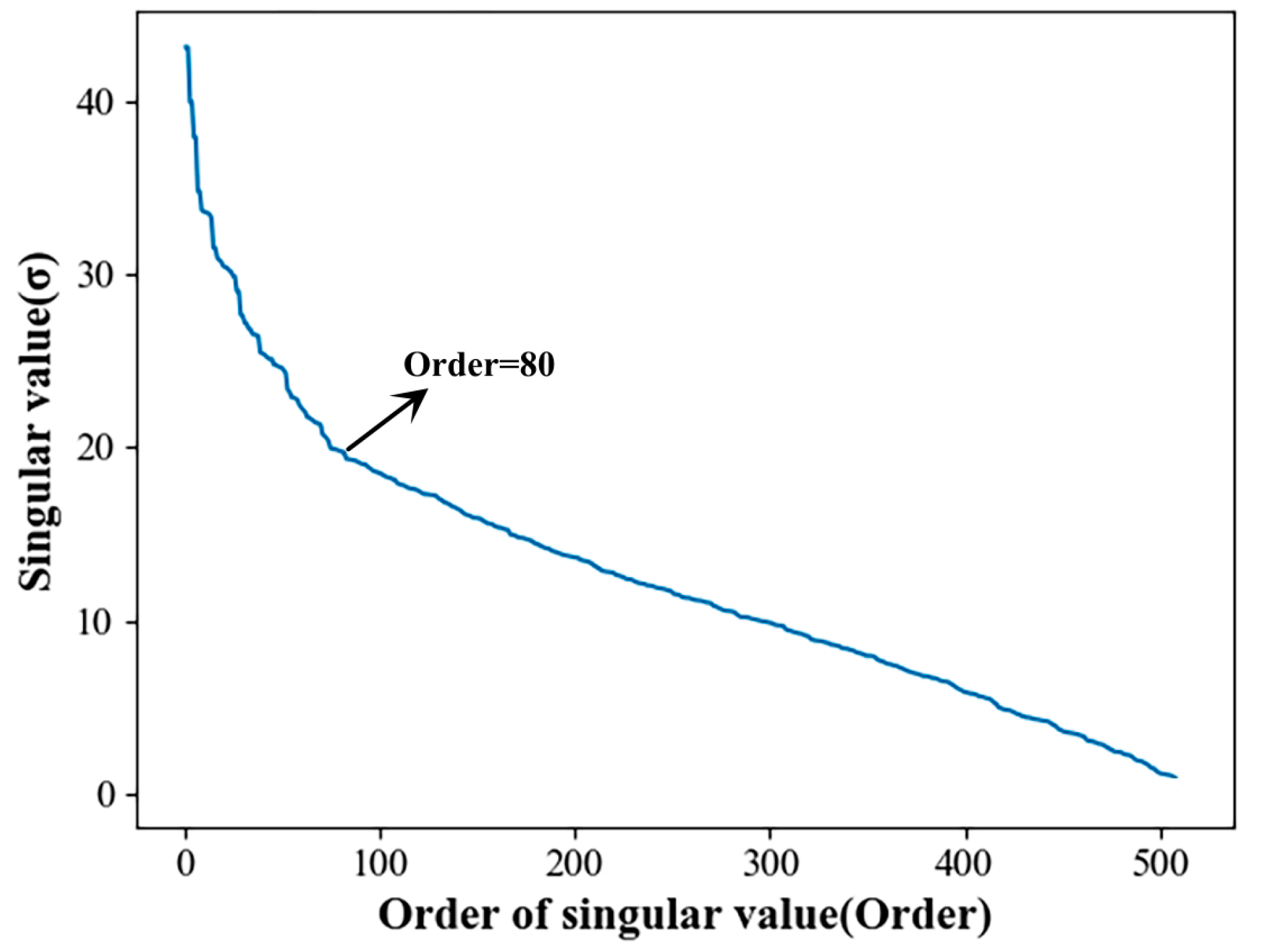
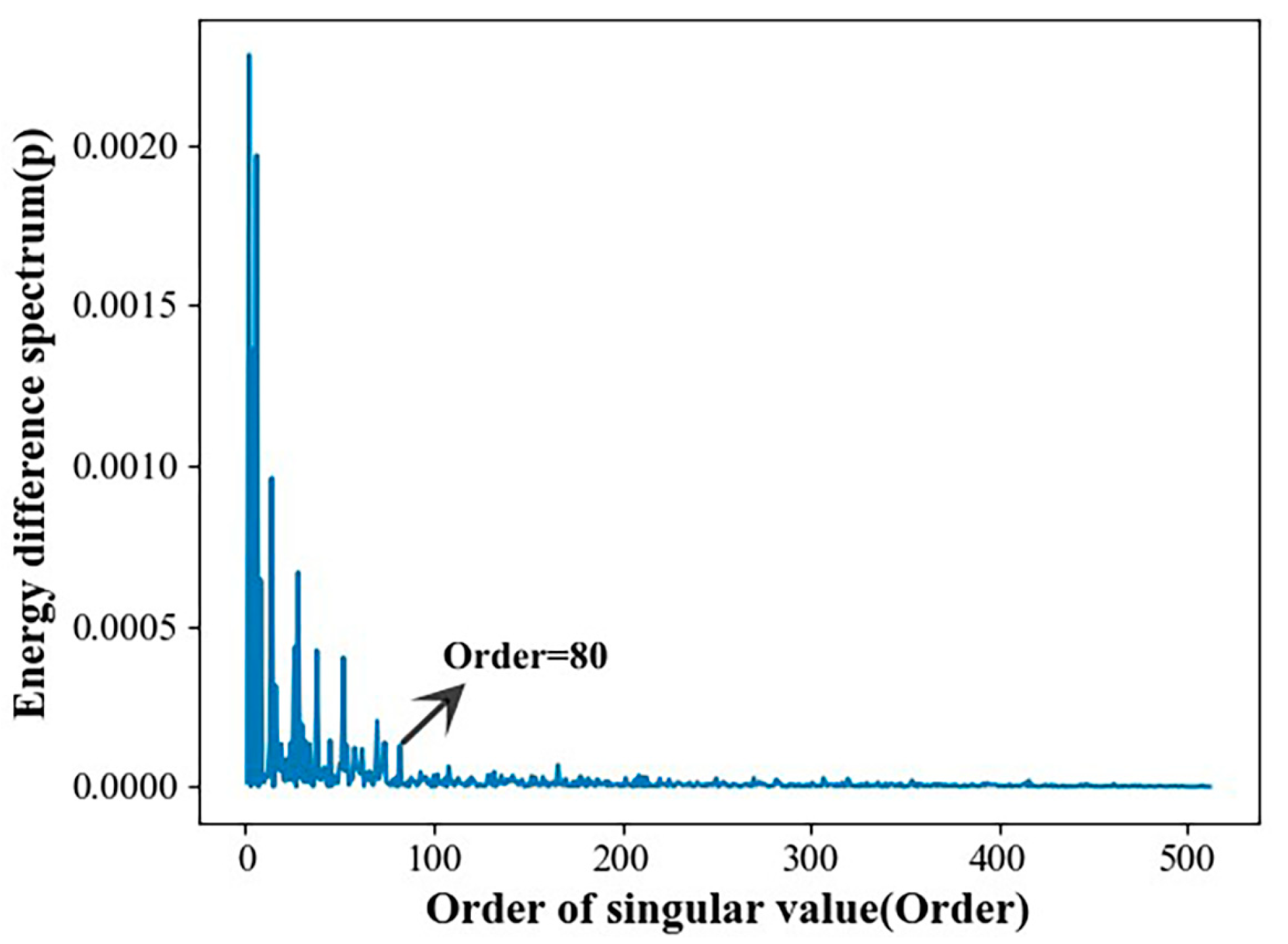
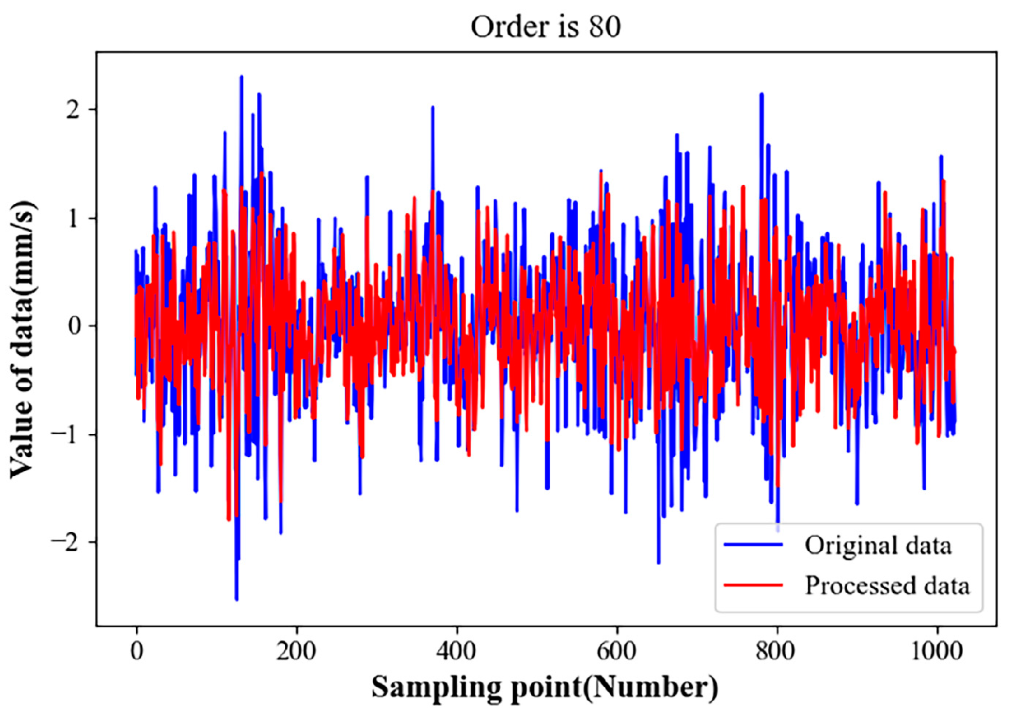
- The SVD algorithm was used to preprocess and denoise the original signal of the gearbox. In terms of SVD signal reconstruction, a singular value energy difference spectrum was introduced. This method determines the effective order of the reconstruction matrix after singular value decomposition based on the contribution of noise signals and useful signals to singular values.
- (3)
- The one-dimensional gearbox vibration signal and the two-dimensional frequency map of STFT time and CNN were combined. CNN multifeature fusion was used to enrich the features of the two different dimensions, which reduced the problem of gearbox information loss during the adaptive extraction process.
2. Principle Introduction
2.1. SVD
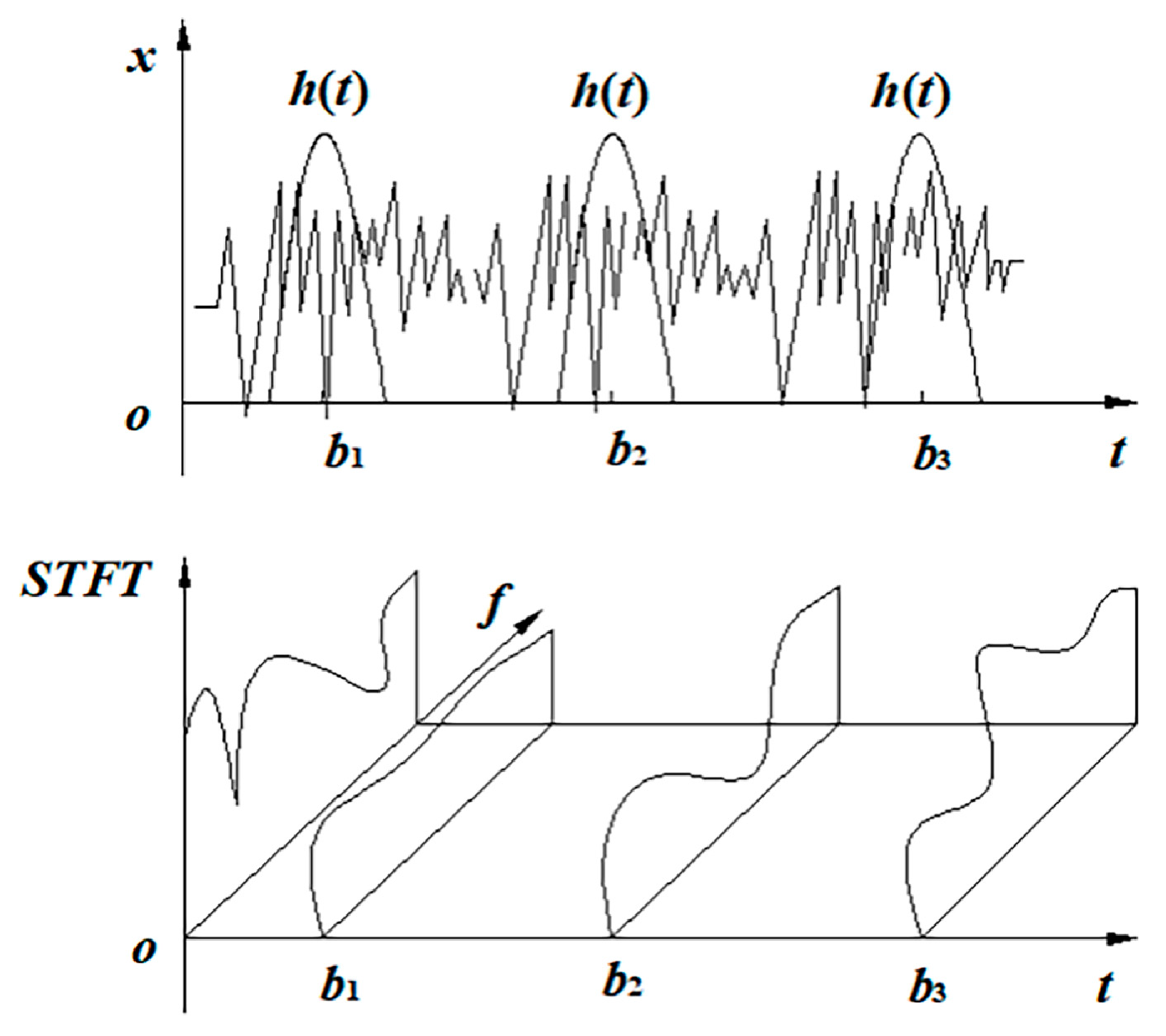
2.2. STFT
2.3. CNN
- (1)
- Input layer. The CNN input layer can preprocess the input data, such as standardization, normalization, etc.
- (2)
- Convolutional layer. The convolutional layer is the core component of CNN. Its largest feature is weight sharing, which can be realized through the convolution kernel. The convolutional layer uses the convolution kernel to locally operate on the input data to extract the corresponding features of this part. As the number of convolutional layers deepens, the required parameters also increase. Deeper features can also be extracted. The convolution operation expression is as follows:In Formula (5), the number of convolutional layers is , the output of the layer is , the input of the layer is , the weight matrix is , the bias is , the activation function used by the convolutional layer is and is the th convolution area of the feature map layer.
- (3)
- Pooling layer. Pooling layers are also called downsampling layers. This layer mainly performs feature extraction and dimensionality reduction during the running of the CNN, which can reduce the amount of calculation required. To a certain extent, it can also reduce the possibility of overfitting. The maximum pooling formula is:In Formula (6), means maximum pooling, the number of pooling layers is , represents the activation value, represents the pooling width, the minimum value of is and the maximum value range is . The -th activation value of the -th eigenvalue of the layer is .
- (4)
- Fully connected layer and output layer. After the previous convolutional and pooling rounds, the fully connected layer of the image input is fully connected between the input and output. This mainly summarizes the features extracted by the convolutional layer and the pooling layer to achieve global optimization [39]. The Softmax function is generally used as the classifier of the output layer. However, as the Softmax classifier leads to insufficient generalization ability of the graphical model and is not suitable for image classification, here we instead use SVM.
2.4. SVM
3. Fault Diagnosis Model Construction
3.1. 1DCNN + 2DCNN + SVM Model
3.2. Multidomain Information Fusion Model
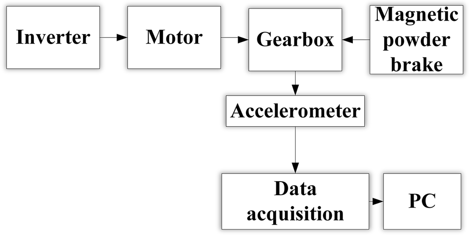
4. Fault Diagnosis Experimental Setup and Data Collection
- (1)
- An air switch was added between the inverter and the power plug to ensure that the experimental process was carried out under safe conditions;
- (2)
- The motor was connected to the frequency converter, and then the gearbox and the motor were connected by a belt. The magnetic powder brake and the gearbox were connected via coupling.
- (3)
- A piezoelectric acceleration sensor was installed at the axial position of the high-speed shaft end cover of the gearbox and was connected to a PC via an acquisition card.
5. Experimental Analysis and Verification
5.1. Gearbox Vibration Signal Preprocessing
5.2. Time–Frequency Map Obtained by STFT
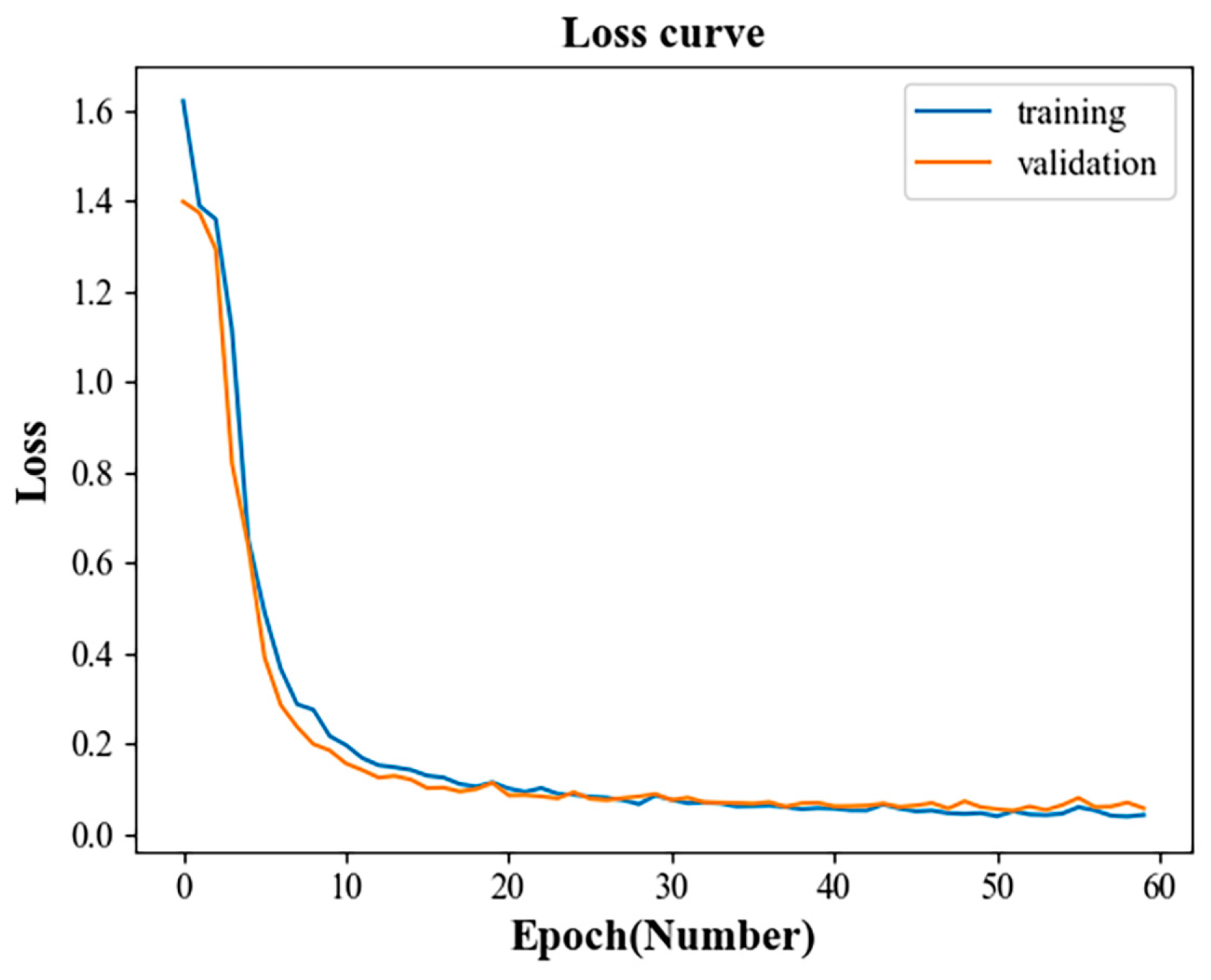
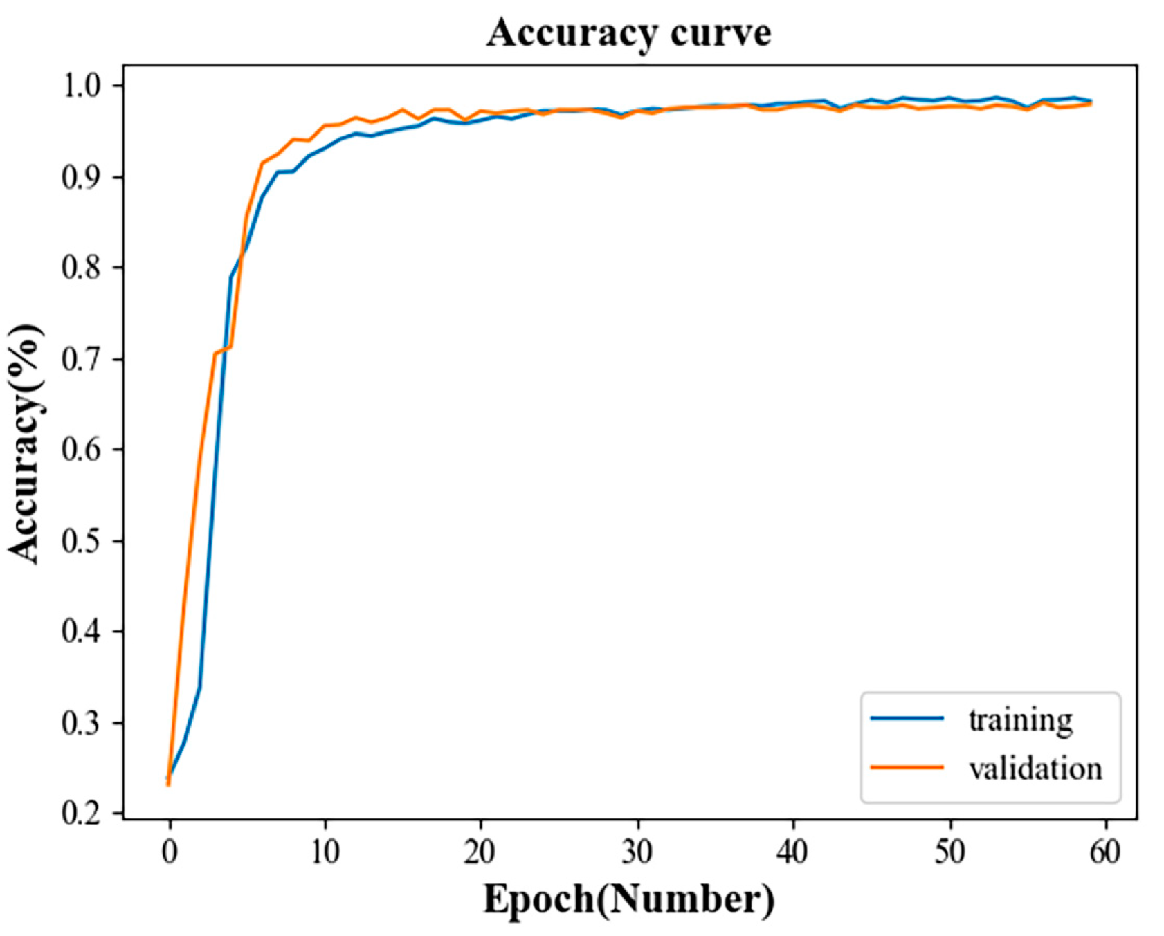
5.3. Overall Model Analysis of Fault Diagnosis
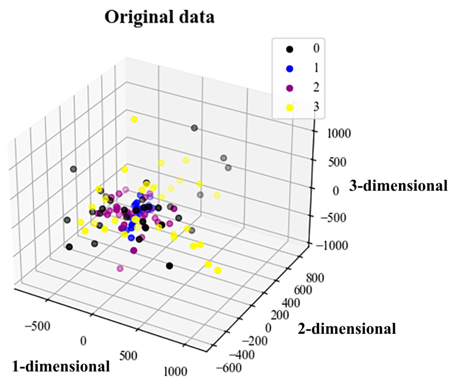
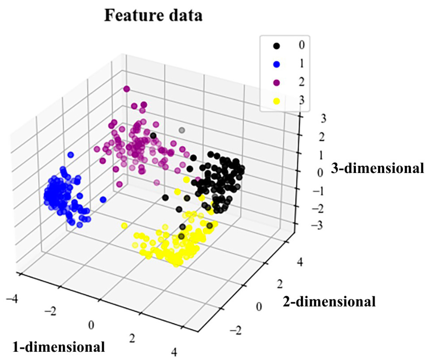
5.4. t-SNE Visualization Algorithm and Analysis
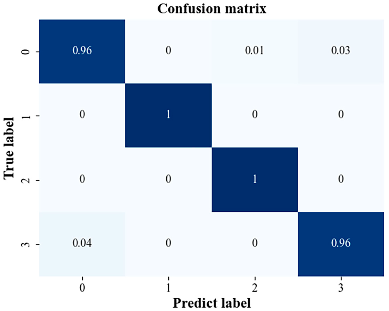
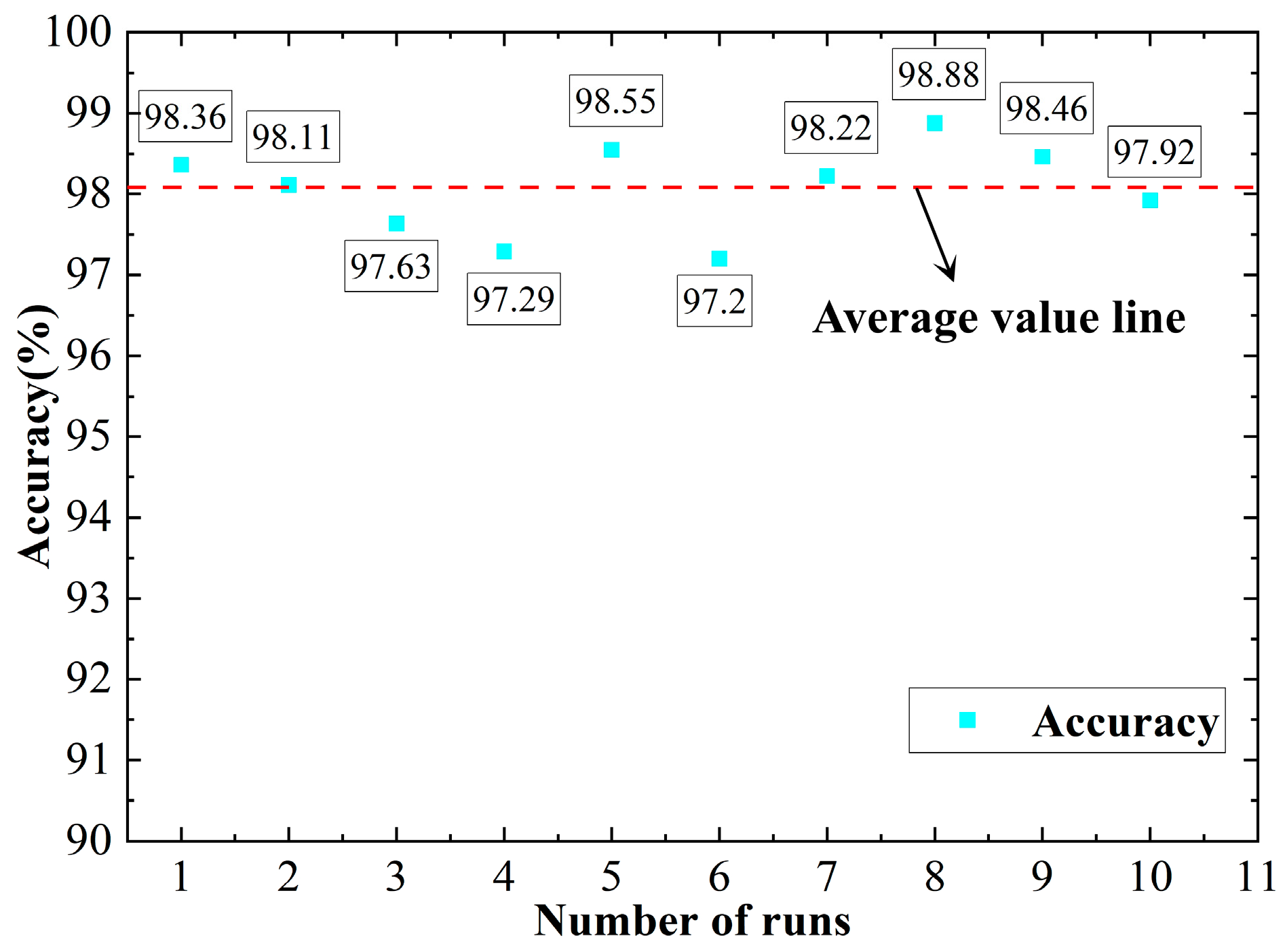
5.5. Result Analysis
5.6. Comparative Analysis
5.6.1. Comparative Analysis of Other Methods
5.6.2. Comparative Analysis of Standard Data Sets
6. Conclusions
- (1)
- The gearbox fault diagnosis method based on a multidomain information fusion CNN model is feasible and effective. The model combines a 1D gearbox vibration signal, an STFT 2D time–frequency map and a CNN. CNN multifeature fusion is used to enrich the features of two different dimensions, and two-channel random features are pooled and fused into a one-dimensional feature array. The extracted features are fully enhanced and fused to achieve the purpose of intelligent gearbox fault diagnosis. The model also avoids the incomplete expression of feature information caused by feature extraction and the low accuracy of traditional pattern recognition methods.
- (2)
- A comparison of the model proposed in this paper with the FFT-2DCNN, 1DCNN-SVM and 2DCNN-SVM models shows that the method proposed in this paper has higher accuracy and stronger generalization ability. In addition, it provides a new conceptualization of a physical model for gearbox fault diagnosis and identification.
- (3)
- In research on the fault diagnosis of future rail vehicle gearboxes, multiple sensors can be sampled for data acquisition and multiphysics domain data fusion in order to improve the accuracy of the diagnostic results.
Author Contributions
Funding
Institutional Review Board Statement
Informed Consent Statement
Data Availability Statement
Conflicts of Interest
References
- Tong, S.; Li, J.; Cong, F.; Fu, Z.; Tong, Z. Vibration Separation Methodology Compensated by Time-Varying Transfer Function for Fault Diagnosis of Non-Hunting Tooth Planetary Gearbox. Sensors 2022, 22, 557. [Google Scholar] [CrossRef] [PubMed]
- Lei, Y.; Lin, J.; Zuo, M.J.; He, Z. Condition monitoring and fault diagnosis of planetary gearboxes: A review. Measurement 2014, 48, 292–305. [Google Scholar] [CrossRef]
- Wang, Z.; Wang, J.; Wang, Y. An intelligent diagnosis scheme based on generative adversarial learning deep neural networks and its application to planetary gearbox fault pattern recognition. Neurocomputing 2018, 310, 213–222. [Google Scholar] [CrossRef]
- Ren, F.; Wang, D.; Shi, G.; Wu, X. Investigation on Dynamic Characteristics of Spur Gear Transmission System with Crack Fault. Machines 2022, 10, 664. [Google Scholar] [CrossRef]
- Zhang, K.; Zhou, T.; Shao, Y.; Wang, G. The influence of time-varying mesh stiffness on natural characteristics of planetary gear system. J. Phys. Conf. Ser. 2021, 1948, 012079. [Google Scholar] [CrossRef]
- Yu, J.; Zhou, X.; Lu, L.; Zhao, Z. Multiscale dynamic fusion global sparse network for gearbox fault diagnosis. IEEE Trans. Instrum. Meas. 2021, 70, 3516111. [Google Scholar] [CrossRef]
- Liu, B.; Riemenschneider, S.; Xu, Y. Gearbox. fault diagnosis using empirical mode decomposition and Hilbert spectrum. Mech. Syst. Signal Process. 2006, 20, 718–734. [Google Scholar] [CrossRef]
- Cheng, J.; Yu, D.; Tang, J.; Yang, Y. Application of SVM and SVD technique based on EMD to the fault diagnosis of the rotating machinery. Shock. Vib. 2009, 16, 89–98. [Google Scholar] [CrossRef]
- Wang, D.-F.; Guo, Y.; Wu, X.; Na, J.; Litak, G. Planetary-Gearbox Fault Classification by Convolutional Neural Network and Recurrence Plot. Appl. Sci. 2020, 10, 932. [Google Scholar] [CrossRef]
- Chen, Z.; Liu, C.; Gryllias, K.; Li, W. Gearbox fault diagnosis using convolutional neural networks and support vector machines. In Proceedings of the 2019 27th European Signal Processing Conference (EUSIPCO), A Coruña, Spain, 2–6 September 2019; IEEE: New York, NY, USA, 2019; pp. 1–5. [Google Scholar]
- Luo, Y.; Baddour, N.; Liang, M. Dynamical modeling and experimental validation for tooth pitting and spalling in spur gears. Mech. Syst. Signal Process. 2019, 119, 155–181. [Google Scholar] [CrossRef]
- Spitas, C.; Spitas, V. Coupled multi-DOF dynamic contact analysis model for the simulation of intermittent gear tooth contacts, impacts and rattling considering backlash and variable torque. Proc. Inst. Mech. Eng. Part C J. Mech. Eng. Sci. 2016, 230, 1022–1047. [Google Scholar] [CrossRef]
- Chaari, F.; Fakhfakh, T.; Haddar, M. Dynamic analysis of a planetary gear failure caused by tooth pitting and cracking. J. Fail. Anal. Prev. 2006, 6, 73–78. [Google Scholar] [CrossRef]
- Theodossiades, S.; Natsiavas, S. Periodic and chaotic dynamics of motor-driven gear-pair systems with backlash. Chaos Solitons Fractals 2001, 12, 2427–2440. [Google Scholar] [CrossRef]
- Lei, Y.; Yang, B.; Jiang, X.; Jia, F.; Li, N.; Nandi, A.K. Applications of machine learning to machine fault diagnosis: A review and roadmap. Mech. Syst. Signal Process. 2020, 138, 106587. [Google Scholar] [CrossRef]
- Xu, X.; Cao, D.; Zhou, Y.; Gao, J. Application of neural network algorithm in fault diagnosis of mechanical intelligence. Mech. Syst. Signal Process. 2020, 141, 106625. [Google Scholar] [CrossRef]
- Tang, S.; Yuan, S.; Zhu, Y. Convolutional neural network in intelligent fault diagnosis toward rotatory machinery. IEEE Access 2020, 8, 86510–86519. [Google Scholar] [CrossRef]
- Jiao, J.; Zhao, M.; Lin, J.; Liang, K. A comprehensive review on convolutional neural network in machine fault diagnosis. Neurocomputing 2020, 417, 36–63. [Google Scholar] [CrossRef]
- Surendran, R.; Khalaf, O.I.; Andres, C. Deep learning based intelligent industrial fault diagnosis model. CMC-Comput. Mater. Contin. 2022, 70, 6323–6338. [Google Scholar] [CrossRef]
- Dong, S.; Wang, P.; Abbas, K. A survey on deep learning and its applications. Comput. Sci. Rev. 2021, 40, 100379. [Google Scholar] [CrossRef]
- Li, X.; Liu, H.; Wang, W.; Zheng, Y.; Lv, H.; Lv, Z. Big data analysis of the internet of things in the digital twins of smart city based on deep learning. Future Gener. Comput. Syst. 2022, 128, 167–177. [Google Scholar] [CrossRef]
- Toldinas, J.; Venčkauskas, A.; Damaševičius, R.; Grigaliūnas, Š.; Morkevičius, N.; Baranauskas, E. A Novel Approach for Network Intrusion Detection Using Multistage Deep Learning Image Recognition. Electronics 2021, 10, 1854. [Google Scholar] [CrossRef]
- Batool, I.; Khan, T.A. Software fault prediction using data mining, machine learning and deep learning techniques: A systematic literature review. Comput. Electr. Eng. 2022, 100, 107886. [Google Scholar] [CrossRef]
- Singh, J.; Azamfar, M.; Ainapure, A.; Lee, J. Deep learning-based cross-domain adaptation for gearbox fault diagnosis under variable speed conditions. Meas. Sci. Technol. 2020, 31, 055601. [Google Scholar] [CrossRef]
- Huang, T.; Zhang, Q.; Tang, X.; Zhao, S.; Lu, X. A novel fault diagnosis method based on CNN and LSTM and its application in fault diagnosis for complex systems. Artif. Intell. Rev. 2022, 55, 1289–1315. [Google Scholar] [CrossRef]
- Tang, Q.; Chai, Y.; Qu, J.; Ren, H. Fisher Discriminative Sparse Representation Based on DBN for Fault Diagnosis of Complex System. Appl. Sci. 2018, 8, 795. [Google Scholar] [CrossRef]
- Zhu, J.; Jiang, Q.; Shen, Y.; Qian, C.; Xu, F.; Zhu, Q. Application of recurrent neural network to mechanical fault diagnosis: A review. J. Mech. Sci. Technol. 2022, 36, 527–542. [Google Scholar] [CrossRef]
- Sun, R.; Yang, Z.; Chen, X.; Tian, S.; Xie, Y. Gear fault diagnosis based on the structured sparsity time-frequency analysis. Mech. Syst. Signal Process. 2018, 102, 346–363. [Google Scholar] [CrossRef]
- Ye, L.; Ma, X.; Wen, C. Rotating Machinery Fault Diagnosis Method by Combining Time-Frequency Domain Features and CNN Knowledge Transfer. Sensors 2021, 21, 8168. [Google Scholar] [CrossRef]
- Zhang, X.; Liu, Z.; Miao, Q.; Wang, L. Bearing fault diagnosis using a whale optimization algorithm-optimized orthogonal matching pursuit with a combined time–frequency atom dictionary. Mech. Syst. Signal Process. 2018, 107, 29–42. [Google Scholar] [CrossRef]
- Li, P.; Yuan, H.; Wang, Y.; Chen, X. Pumping unit fault analysis method based on wavelet transform time-frequency diagram and cnn. Int. Core J. Eng. 2020, 6, 182–188. [Google Scholar]
- Fan, H.; Xue, C.; Zhang, X.; Cao, X.; Gao, S.; Shao, S. Vibration images-driven fault diagnosis based on CNN and transfer learning of rolling bearing under strong noise. Shock. Vib. 2021, 2021, 6616592. [Google Scholar] [CrossRef]
- Sadek, R.A. SVD based image processing applications: State of the art, contributions and research challenges. arXiv 2012, arXiv:1211.7102. [Google Scholar]
- Lin, P.; Peng, S.; Zhao, J.; Cui, X. Diffraction separation and imaging using multichannel singular-spectrum analysis. Geophysics 2020, 85, V11–V24. [Google Scholar] [CrossRef]
- Jiang, H.; Chen, J.; Dong, G.; Liu, T.; Chen, G. Study on Hankel matrix-based SVD and its application in rolling element bearing fault diagnosis. Mech. Syst. Signal Process. 2015, 52, 338–359. [Google Scholar] [CrossRef]
- Mustafa, D.; Yicheng, Z.; Minjie, G.; Jonas, H.; Jürgen, F. Motor current based misalignment diagnosis on linear axes with short-time Fourier transform (STFT). Procedia CIRP 2022, 106, 239–243. [Google Scholar] [CrossRef]
- Syed, S.H.; Muralidharan, V. Feature extraction using Discrete Wavelet Transform for fault classification of planetary gearbox–A comparative study. Appl. Acoust. 2022, 188, 108572. [Google Scholar] [CrossRef]
- Wang, J.; Yang, J.; Wang, Y.; Bai, Y.; Zhang, T.; Yao, D. Ensemble decision approach with dislocated time–frequency representation and pre-trained CNN for fault diagnosis of railway vehicle gearboxes under variable conditions. Int. J. Rail Transp. 2022, 10, 655–673. [Google Scholar] [CrossRef]
- Xu, G.; Liu, M.; Jiang, Z.; Shen, W.; Huang, C. Online fault diagnosis method based on transfer convolutional neural networks. IEEE Trans. Instrum. Meas. 2019, 69, 509–520. [Google Scholar] [CrossRef]
- Wang, Y.; Huang, S.; Dai, J.; Tang, J. A novel bearing fault diagnosis methodology based on SVD and one-dimensional convolutional neural network. Shock. Vib. 2020, 2020, 1850286. [Google Scholar] [CrossRef]
- Gong, W.; Chen, H.; Zhang, Z.; Zhang, M.; Wang, R.; Guan, C.; Wang, Q. A Novel Deep Learning Method for Intelligent Fault Diagnosis of Rotating Machinery Based on Improved CNN-SVM and Multichannel Data Fusion. Sensors 2019, 19, 1693. [Google Scholar] [CrossRef]
- Wang, T.; Dong, J.; Xie, T.; Diallo, D.; Benbouzid, M. A Self-Learning Fault Diagnosis Strategy Based on Multi-Model Fusion. Information 2019, 10, 116. [Google Scholar] [CrossRef]
- Kumar, V.; Mukherjee, S.; Verma, A.K.; Sarangi, S. An AI-Based Nonparametric Filter Approach for Gearbox Fault Diagnosis. IEEE Trans. Instrum. Meas. 2022, 71, 3516611. [Google Scholar] [CrossRef]
- Yu, G. A concentrated time–frequency analysis tool for bearing fault diagnosis. IEEE Trans. Instrum. Meas. 2019, 69, 371–381. [Google Scholar] [CrossRef]
- Liu, J.; Li, Q.; Yang, H.; Han, Y.; Jiang, S.; Chen, W. Sequence fault diagnosis for PEMFC water management subsystem using deep learning with t-SNE. IEEE Access 2019, 7, 92009–92019. [Google Scholar] [CrossRef]


| Channel | Network Layer | Convolution Kernel Size @ Step Size | Activation Function |
|---|---|---|---|
| Channel 1 | Input | 64 × 64 | |
| Conv2D-1 | 64 × 64@6 | ReLU | |
| MaxPooling2D-1 | 32 × 32@6 | ||
| Conv2D-2 | 32 × 32@8 | ReLU | |
| MaxPooling2D-2 | 16 × 16@8 | ||
| Conv2D-3 | 16 × 16@12 | ReLU | |
| MaxPooling2D-3 | 8 × 8@12 | ||
| Dropout | 0.5 | ||
| FC1 | 1 × 768 | ||
| Channel 2 | Input | 1 × 1024 | |
| Conv1D-1 | 1 × 1024@6 | ReLU | |
| MaxPooling1D-1 | 1 × 512@6 | ||
| Conv1D-2 | 1 × 512@8 | ReLU | |
| MaxPooling1D-2 | 1 × 256@8 | ||
| Conv1D-3 | 1 × 256@12 | ReLU | |
| MaxPooling1D-3 | 1 × 128@12 | ||
| Dropout | 0.5 | ||
| FC2 | 1 × 1536 | ||
| Fusion | Concatenate | 1 × 2304 | |
| FC3 | 1 × 128 | ReLU | |
| FC4 | 1 × 4 |
| Type | Gearbox Status | Data Length | Motor Speed/r/min | Number of Data Groups |
|---|---|---|---|---|
| 1 | Pitting | 1024 | 900 | 1000 |
| 2 | Broken | 1024 | 900 | 1000 |
| 3 | Wear | 1024 | 900 | 1000 |
| 4 | Normal | 1024 | 900 | 1000 |
| Gearbox Status | Number of Training Sets | Number of Validation Sets | Number of Test Sets | Label |
|---|---|---|---|---|
| Pitting | 700 | 200 | 100 | 0 |
| Broken | 700 | 200 | 100 | 1 |
| Wear | 700 | 200 | 100 | 2 |
| Normal | 700 | 200 | 100 | 3 |
| Total number of samples | 2800 | 800 | 400 |
| Diagnosis Method | FFT-2DCNN | 1DCNN-SVM | 2DCNN-SVM | Multidomain Information Fusion CNN Model |
|---|---|---|---|---|
| Ten times average classification accuracy/% | 93.62 | 90.65 | 94.52 | 98.08 |
| Standard deviation/% | 2.2866 | 2.3798 | 0.9231 | 0.5223 |
| Gearbox Status | Fault Diameter/in | Number of Training Sets | Number of Validation Sets | Number of Test Sets |
|---|---|---|---|---|
| Inner race fault | 0.007 | 700 | 200 | 100 |
| 0.014 | 700 | 200 | 100 | |
| 0.021 | 700 | 200 | 100 | |
| Rolling element failure | 0.007 | 700 | 200 | 100 |
| 0.014 | 700 | 200 | 100 | |
| 0.021 | 700 | 200 | 100 | |
| Outer race fault | 0.007 | 700 | 200 | 100 |
| 0.014 | 700 | 200 | 100 | |
| 0.021 | 700 | 200 | 100 | |
| Normal | normal | 700 | 200 | 100 |
| Diagnosis Method | FFT-2DCNN | 1DCNN-SVM | 2DCNN-SVM | Multidomain Information Fusion CNN Model |
|---|---|---|---|---|
| Ten times average classification accuracy/% | 95.24 | 92.37 | 96.85 | 99.28 |
| Standard deviation/% | 1.7625 | 1.9236 | 0.8264 | 0.3579 |
Disclaimer/Publisher’s Note: The statements, opinions and data contained in all publications are solely those of the individual author(s) and contributor(s) and not of MDPI and/or the editor(s). MDPI and/or the editor(s) disclaim responsibility for any injury to people or property resulting from any ideas, methods, instructions or products referred to in the content. |
© 2023 by the authors. Licensee MDPI, Basel, Switzerland. This article is an open access article distributed under the terms and conditions of the Creative Commons Attribution (CC BY) license (https://creativecommons.org/licenses/by/4.0/).
Share and Cite
Xie, F.; Wang, G.; Shang, J.; Liu, H.; Xiao, Q.; Xie, S. Gearbox Fault Diagnosis Method Based on Multidomain Information Fusion. Sensors 2023, 23, 4921. https://doi.org/10.3390/s23104921
Xie F, Wang G, Shang J, Liu H, Xiao Q, Xie S. Gearbox Fault Diagnosis Method Based on Multidomain Information Fusion. Sensors. 2023; 23(10):4921. https://doi.org/10.3390/s23104921
Chicago/Turabian StyleXie, Fengyun, Gan Wang, Jiandong Shang, Hui Liu, Qian Xiao, and Sanmao Xie. 2023. "Gearbox Fault Diagnosis Method Based on Multidomain Information Fusion" Sensors 23, no. 10: 4921. https://doi.org/10.3390/s23104921
APA StyleXie, F., Wang, G., Shang, J., Liu, H., Xiao, Q., & Xie, S. (2023). Gearbox Fault Diagnosis Method Based on Multidomain Information Fusion. Sensors, 23(10), 4921. https://doi.org/10.3390/s23104921