
Smooth Autonomous Patrolling for a Differential-Drive Mobile Robot in Dynamic Environments


Abstract
:1. Introduction
- •
- The development of a complete autonomous navigation system for differential-drive mobile robots;
- •
- The development of a combined global and local planner for fast path replanning in dynamic environments;
- •
- The realization of real-time traversable collision-free path planning based on clothoids;
- •
- The realization of orientation alignment using the golden ratio.
2. Theoretical Background
- Perception—Sensors, e.g., GPS, encoders, IMU, 3D laser, cameras, etc., are used for collecting information from the environment for different applications, e.g., mobile robot localization, the mapping of the environment, and object or human tracking;
- Localization—The determination of a robot’s position in a global coordinate frame;
- Path planning and smoothing—Finding a feasible, smooth, collision-free path from the starting point to the goal point;
- Motion control—While respecting the actuator-related limits of the robot, the robot’s motions are controlled to ensure that it follows the desired trajectory.
2.1. Environment Model and Search Graph
2.2. Path Planning
Path Continuity
2.3. Path Smoothing
Feasible Paths
- A holonomic constraint—The wheels of the robot must roll and cannot slip:
- The minimum turning radius of the robot is lower-bounded by the value , and curvature is upper-bounded by .
- , where , , and , where the configuration space of the mobile robot is expressed as ; is free configuration space without obstacles; and l is the length of the clothoid at the goal configuration;
- The curvature profile is a continuous function ;
- The smooth path is collision-free: where is a set of obstacles.
2.4. Motion Control
2.4.1. Trajectory Planning
2.4.2. Trajectory Tracking
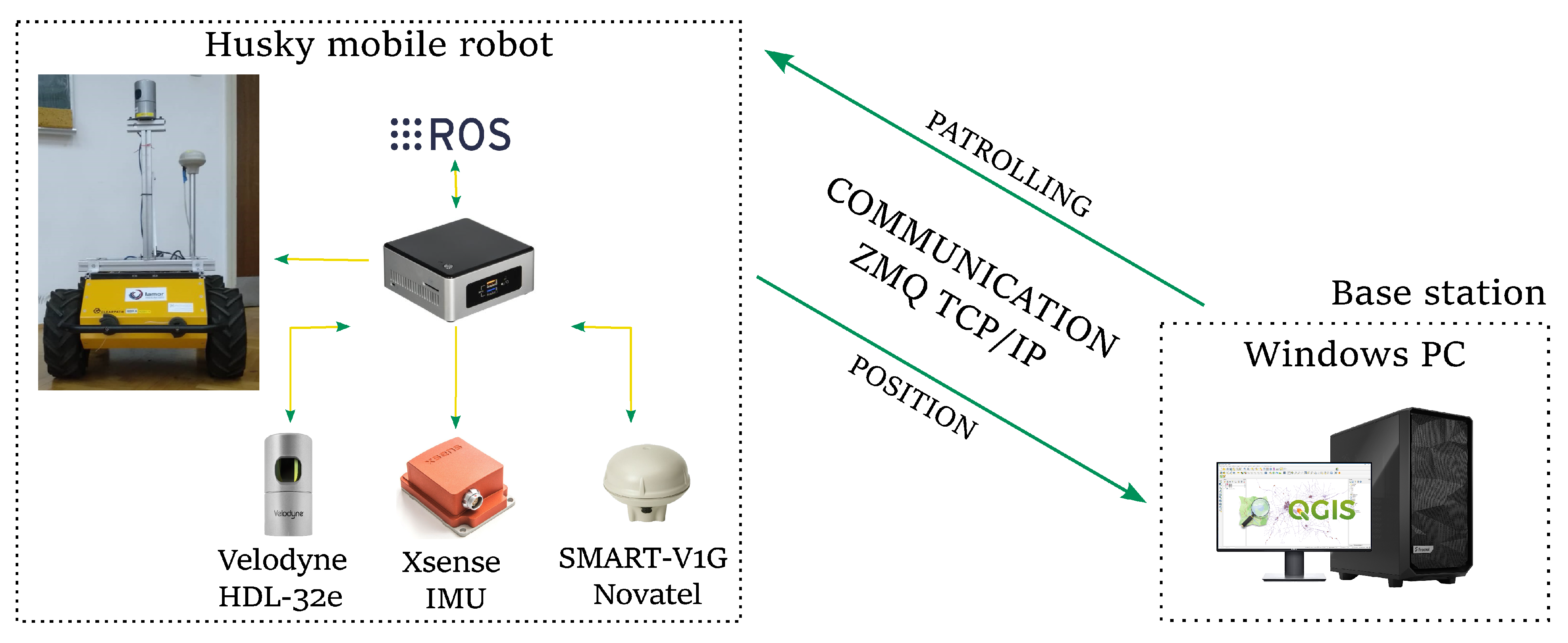
3. Control System Architecture
3.1. Task Assignment and Supervision
3.2. QGIS and ROS Communication
3.3. Autonomous Navigation System
4. Smooth-Motion-Planning Scheme
4.1. Global Planner
4.2. Obstacle Detection
| Algorithm 1 Obstacle detection |
|
4.3. Local Planner
4.4. Orientation Alignment
- 1.
- Determine the angle as the direction of the first segment on the replanned TWD* path.
- 2.
- Compute the absolute angular difference between the robot’s current orientation and the angle . There are two possible cases: (i) 0° < 90° and (ii) 90° < 180°.
- 3.
- For case (i), two additional points, , must be calculated (see Figure 5a). First point is always in the direction of the robot’s orientation and is at a distance of from the robot’s current position. is equal to the diameter of the circumscribed circle around the robot’s footprint. The second point is on the first segment of the replanned TWD* path determined using the golden ratio rule (13). For case (ii), three additional points, , must be calculated (see Figure 5b). The procedure for calculating the first and third points is the same as for points in the previous case. An additional point is added in the direction of the robot’s orientation minus 90° to reduce this case to the previous case.
| Algorithm 2 Orientation alignment |
|
4.5. Path Smoothing
4.6. Velocity Profile Optimization
4.7. Trajectory Tracking
5. Simulation Results
- Path length (L)—calculated via the summation of the Euclidean distance between sampling points on the path;
- Execution time (T)—calculated via the summation of the discretization time required to travel between sampling points on the path;
- Tracking error ()—the deviation of the tracked trajectory from the patrolling route, which is determined as a surface between these two curves based on the trapezoidal rule;
- Average acceleration ()—calculated via the summation of acceleration values at each point on the trajectory;
- Average curvature ()—calculated via the summation of all curvature values at each point on the trajectory;
- Initial path-planning time ()—calculated via the average measured time required for ten algorithm executions.
5.1. Smooth Motion Planning without Replanning
- Bending energy (BE)—calculated via the summation of the squares of the curvature at each point of the trajectory:where is the curvature at each point of the robot trajectory and n is the number of points in the trajectory [36].
- Curvature variation energy (CVE)—calculated via the summation of the squares of the change in the curvature in the trajectory, i.e., the sharpness at each point of the trajectory:
5.2. Smooth Motion Planning with Replanning
6. Experimental Results
6.1. Smooth Motion Planning without Replanning
6.2. Smooth Motion Planning with Replanning
7. Limitations and Recommendations for Improvement
7.1. Hardware Limitation
7.2. Obstacle Detection
7.3. The Velocity of Obstacle
7.4. Trade-Off between Path Planning Time and Accuracy
7.5. Different Mobile Robots
8. Conclusions
Author Contributions
Funding
Institutional Review Board Statement
Informed Consent Statement
Data Availability Statement
Conflicts of Interest
References
- Farooq, M.U.; Eizad, A.; Bae, H.K. Power solutions for autonomous mobile robots: A survey. Robot. Auton. Syst. 2023, 159, 104285. [Google Scholar] [CrossRef]
- Azpúrua, H.; Saboia, M.; Freitas, G.M.; Clark, L.; Agha-mohammadi, A.A.; Pessin, G.; Campos, M.F.; Macharet, D.G. A Survey on the autonomous exploration of confined subterranean spaces: Perspectives from real-word and industrial robotic deployments. Robot. Auton. Syst. 2023, 160, 104304. [Google Scholar] [CrossRef]
- Couillard, M.; Fawcett, J.; Davison, M. Optimizing Constrained Search Patterns for Remote Mine-Hunting Vehicles. IEEE J. Ocean. Eng. 2012, 37, 75–84. [Google Scholar] [CrossRef]
- Abouaf, J. Trial by fire: Teleoperated robot targets Chernobyl. IEEE Comput. Graph. Appl. 1998, 18, 10–14. [Google Scholar] [CrossRef]
- Hoshino, S.; Ishiwata, T.; Ueda, R. Optimal patrolling methodology of mobile robot for unknown visitors. Adv. Robot. 2016, 30, 1072–1085. [Google Scholar] [CrossRef]
- Chen, X. Fast Patrol Route Planning in Dynamic Environments. IEEE Trans. Syst. Man Cybern.—Part A Syst. Hum. 2012, 42, 894–904. [Google Scholar] [CrossRef]
- Czarnowski, J.; Dąbrowski, A.; Maciaś, M.; Główka, J.; Wrona, J. Technology gaps in human-machine interfaces for autonomous construction robots. Autom. Constr. 2018, 94, 179–190. [Google Scholar] [CrossRef]
- Nohel, J.; Stodola, P.; Flasar, Z. Combat UGV Support of Company Task Force Operations. In Proceedings of the International Conference on Modelling and Simulation for Autonomous Systems, Virtual Event, 13–14 October 2021; pp. 29–42. [Google Scholar] [CrossRef]
- Teh, C.K.; Kit Wong, W.; Min, T.S. Extended Dijkstra Algorithm in Path Planning for Vision Based Patrol Robot. In Proceedings of the 2021 8th International Conference on Computer and Communication Engineering (ICCCE), Kuala Lumpur, Malaysia, 22–23 June 2021; pp. 184–189. [Google Scholar] [CrossRef]
- Ma, J.; Hu, L.; Pan, B.; Li, Z.; Tian, Y.; Chen, C. Analysis and Decision of Optimal Path of Forest Disaster Patrol Based on Beidou Navigation. In Proceedings of the 2020 39th Chinese Control Conference (CCC), Shenyang, China, 27–29 July 2020; pp. 5624–5629. [Google Scholar] [CrossRef]
- Gao, H.; Ma, Z.; Zhao, Y. A Fusion Approach for Mobile Robot Path Planning Based on Improved A* Algorithm and Adaptive Dynamic Window Approach. In Proceedings of the 2021 IEEE 4th International Conference on Electronics Technology (ICET), Chengdu, China, 7–10 May 2021; pp. 882–886. [Google Scholar] [CrossRef]
- Fox, D.; Burgard, W.; Thrun, S. The dynamic window approach to collision avoidance. IEEE Robot. Autom. Mag. 1997, 4, 23–33. [Google Scholar] [CrossRef]
- Seder, M.; Macek, K.; Petrovic, I. An Integrated Approach to Real-Time Mobile Robot Control in Partially Known Indoor Environments. In Proceedings of the Annual Conference of the IEEE Industrial Electronics Society, Raleigh, NC, USA, 6–10 November 2005. [Google Scholar] [CrossRef]
- Kim, D.; Shin, S. Local path planning using a new artificial potential function composition and its analytical design guidelines. Adv. Robot. 2006, 20, 115–135. [Google Scholar] [CrossRef]
- Stentz, A. Optimal and efficient path planning for partially-known environments. In Proceedings of the 1994 IEEE International Conference on Robotics and Automation, San Diego, CA, USA, 8–13 May 1994; Volume 4, pp. 3310–3317. [Google Scholar] [CrossRef]
- Seder, M.; Petrović, I. Two-way D* algorithm for path planning and replanning. Robot. Auton. Syst. 2011, 59, 329–342. [Google Scholar] [CrossRef]
- Li, X.; Choi, B.J. Design of obstacle avoidance system for mobile robot using fuzzy logic systems. Int. J. Smart Home 2013, 7, 321–328. [Google Scholar]
- Gong, C.; Li, Z.; Zhou, X.; Li, J.; Zhou, J.; Gong, J. Orientation-Aware Planning for Parallel Task Execution of Omni-Directional Mobile Robot. In Proceedings of the 2021 IEEE/RSJ International Conference on Intelligent Robots and Systems (IROS), Prague, Czech Republic, 27 September–1 October 2021; pp. 6891–6898. [Google Scholar] [CrossRef]
- Jing, X.J. Behavior dynamics based motion planning of mobile robots in uncertain dynamic environments. Robot. Auton. Syst. 2005, 53, 99–123. [Google Scholar] [CrossRef]
- Dubin, L.E. On curves of minimal length with constraint on average curvature, and with prescribed initial and terminal positions and tangents. Am. J. Math. 1957, 79, 497–516. [Google Scholar] [CrossRef]
- Yu, X.; Roppel, T.A.; Hung, J.Y. An Optimization Approach for Planning Robotic Field Coverage. In Proceedings of the 41st Annual Conference of the IEEE Inductrial Electronics Society, Yokohama, Japan, 9–12 November 2015. [Google Scholar] [CrossRef]
- Song, B.; Tian, G.; Zhou, F. A comparison study on path smoothing algorithms for laser robot navigated mobile robot path planning in intelligent space. J. Inf. Comput. Sci. 2010, 7, 2943–2950. [Google Scholar]
- Elbanhawi, M.; Simic, M.; Jazar, R.N. Continuous Path Smoothing for Car-Like Robots Using B-Spline Curves. J. Intell. Robot. Syst. 2015, 80, 23–56. [Google Scholar] [CrossRef]
- Yang, K.; Jung, D.; Sukkarieh, S. Continuous curvature path-smoothing algorithm using cubic B zier spiral curves for non-holonomic robots. Adv. Robot. 2013, 27, 247–258. [Google Scholar] [CrossRef]
- Zhang, B.; Liu, D.; Liu, L.; Zhao, Y.; Sun, L.; Yao, Z. Path Prediction Method for Automotive Applications Based on Cubic Spline Interpolation. In Proceedings of the 2022 International Conference on Advanced Robotics and Mechatronics (ICARM), Tokyo, Japan, 21–22 July 2022; pp. 1086–1091. [Google Scholar] [CrossRef]
- Luka, K.; Žubrinić, D.; Županović, V. Box dimension and minkowski content of the clothoid. Fractals-Complex Geom. Patterns Scaling Nat. Soc. FRACTALS 2009, 17, 485–492. [Google Scholar] [CrossRef]
- Brezak, M.; Petrović, I. Real-time Approximation of Clothoids With Bounded Error for Path Planning Applications. IEEE Trans. Robot. 2014, 30, 507–515. [Google Scholar] [CrossRef]
- Seder, M.; Jurić, A.; Šelek, A.; Marić, F.; Lovrić, M.; Petrović, I. Autonomous navigation of a tracked unmanned ground vehicle. IFAC-PapersOnLine 2022, 55, 120–125. [Google Scholar] [CrossRef]
- Klančar, G.; Seder, M. Combined stochastic-deterministic predictive control using local-minima free navigation. In Proceedings of the 2021 IEEE/RSJ International Conference on Intelligent Robots and Systems (IROS), Prague, Czech Republic, 27 September–1 October 2021; pp. 5788–5793. [Google Scholar] [CrossRef]
- Mac, T.T.; Copot, C.; Tran, D.T.; De Keyser, R. Heuristic approaches in robot path planning: A survey. Robot. Auton. Syst. 2016, 86, 13–28. [Google Scholar] [CrossRef]
- Thrun, S.; Burgard, W.; Fox, D. Probabilistic Robotics (Intelligent Robotics and Autonomous Agents); The MIT Press: Cambridge, MA, USA, 2005. [Google Scholar]
- Ravankar, A.; Ravankar, A.A.; Kobayashi, Y.; Hoshino, Y.; Peng, C.C. Path Smoothing Techniques in Robot Navigation: State-of-the-Art, Current and Future Challenges. Sensors 2018, 18, 3170. [Google Scholar] [CrossRef] [PubMed]
- Lepetič, M.; Klančar, G.; Škrjanc, I.; Matko, D.; Potočnik, B. Time optimal path planning considering acceleration limits. Robot. Auton. Syst. 2003, 45, 199–210. [Google Scholar] [CrossRef]
- Šelek, A.; Jurić, D.; Čirjak, A.; Marić, F.; Seder, M.; Marković, I.; Petrović, I. Control architecture of a remotely controlled vehicle in extreme CBRNE conditions. In Proceedings of the 2019 International Conference on Electrical Drives Power Electronics (EDPE), The High Tatras, Slovakia, 24–26 September 2019; pp. 273–278. [Google Scholar] [CrossRef]
- Kanayama, Y.; Kimura, Y.; Miyazaki, F.; Noguchi, T. A stable tracking control method for an autonomous mobile robot. In Proceedings of the IEEE International Conference on Robotics and Automation, Cincinnati, OH, USA, 13–18 May 1990; Volume 1, pp. 384–389. [Google Scholar] [CrossRef]
- Gobithaasan, R.; Yip, S.; Miura, K.; Shanmugavel, M. Optimal Path Smoothing with Log-aesthetic Curves Based on Shortest Distance, Minimum Bending Energy or Curvature Variation Energy. Comput.-Aided Des. Appl. 2019, 17, 639–658. [Google Scholar] [CrossRef]


| Original Method | Proposed Method | |
|---|---|---|
| L [m] | 25.21 | 22.55 |
| T [s] | 61.8 | 51.6 |
| [m] | 4.32 | 3.67 |
| [m/s] | 0.24 | 0.08 |
| [m] | 0.94 | 0.24 |
| [ms] | 407.56 | 6.27 |
| Smoothing Method | L [m] | T [s] | [m] | [m] | BE | CVE |
|---|---|---|---|---|---|---|
| Clothoid | 22.55 | 47.16 | 3.48 | 0.25 | 0.14 | 0.25 |
| B-spline | 27.79 | 60.59 | 6.05 | 0.84 | 5.55 | 20.21 |
| Bézier curve | 25.97 | 54.66 | 8.25 | 0.44 | 0.28 | 1.67 |
| Cubic spline | 24.93 | 51.87 | 3.82 | 0.29 | 0.13 | 0.11 |
| Cubic Hermit spline | 25.28 | 53.96 | 3.48 | 0.40 | 0.35 | 4.16 |
| Dubins curve | 24.98 | 54.18 | 4.28 | 0.68 | 0.24 | 2.88 |
| Method | L [m] | T [s] | [m/s] | [m] | [ms] |
|---|---|---|---|---|---|
| STWD* | 10.70 | 24.20 | 0.13 | 0.47 | 369.15 |
| APF | 13.17 | 26.72 | 0.13 | 0.55 | 24.58 |
| DWA | 12.07 | 24.45 | 0.12 | 0.39 | 49.45 |
| MPC | 10.93 | 24.40 | 0.08 | 0.65 | 27.35 |
| Original Method | Proposed Method | |
|---|---|---|
| L [m] | 14.90 | 13.77 |
| T [s] | 61.18 | 40.07 |
| [m] | 1.89 | 0.68 |
| [m/s] | 0.27 | 0.25 |
| [m] | 0.58 | 0.49 |
| [ms] | 46.26 | 4.27 |
Disclaimer/Publisher’s Note: The statements, opinions and data contained in all publications are solely those of the individual author(s) and contributor(s) and not of MDPI and/or the editor(s). MDPI and/or the editor(s) disclaim responsibility for any injury to people or property resulting from any ideas, methods, instructions or products referred to in the content. |
© 2023 by the authors. Licensee MDPI, Basel, Switzerland. This article is an open access article distributed under the terms and conditions of the Creative Commons Attribution (CC BY) license (https://creativecommons.org/licenses/by/4.0/).
Share and Cite
Šelek, A.; Seder, M.; Petrović, I. Smooth Autonomous Patrolling for a Differential-Drive Mobile Robot in Dynamic Environments. Sensors 2023, 23, 7421. https://doi.org/10.3390/s23177421
Šelek A, Seder M, Petrović I. Smooth Autonomous Patrolling for a Differential-Drive Mobile Robot in Dynamic Environments. Sensors. 2023; 23(17):7421. https://doi.org/10.3390/s23177421
Chicago/Turabian StyleŠelek, Ana, Marija Seder, and Ivan Petrović. 2023. "Smooth Autonomous Patrolling for a Differential-Drive Mobile Robot in Dynamic Environments" Sensors 23, no. 17: 7421. https://doi.org/10.3390/s23177421
APA StyleŠelek, A., Seder, M., & Petrović, I. (2023). Smooth Autonomous Patrolling for a Differential-Drive Mobile Robot in Dynamic Environments. Sensors, 23(17), 7421. https://doi.org/10.3390/s23177421