
Fault Detection in 3D Printing: A Study on Sensor Positioning and Vibrational Patterns


Abstract
:1. Introduction
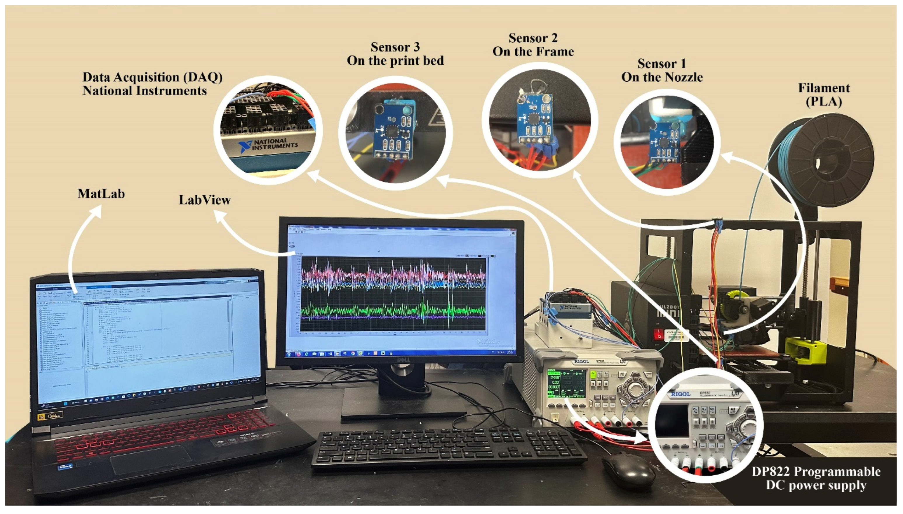
2. Materials and Methods
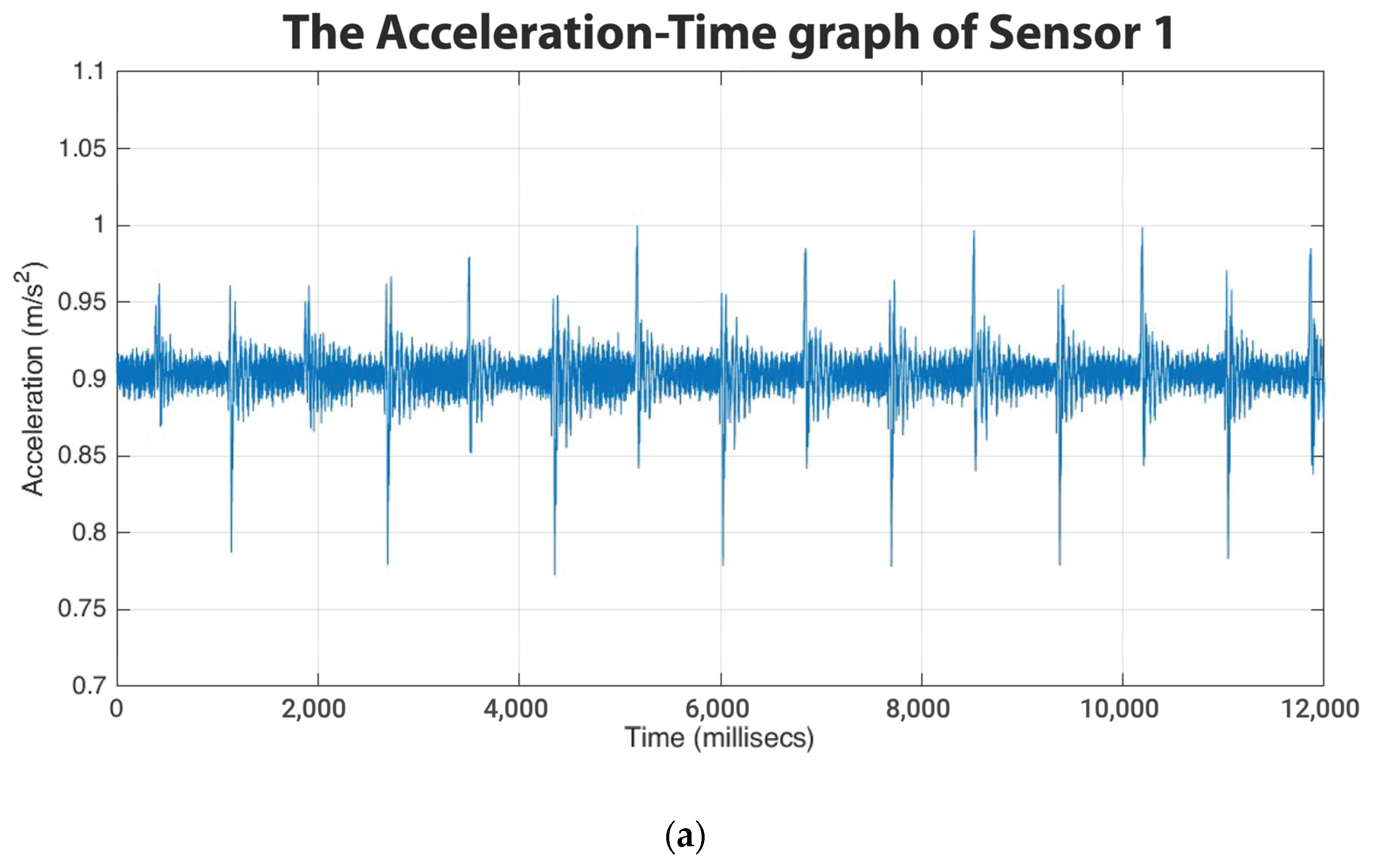
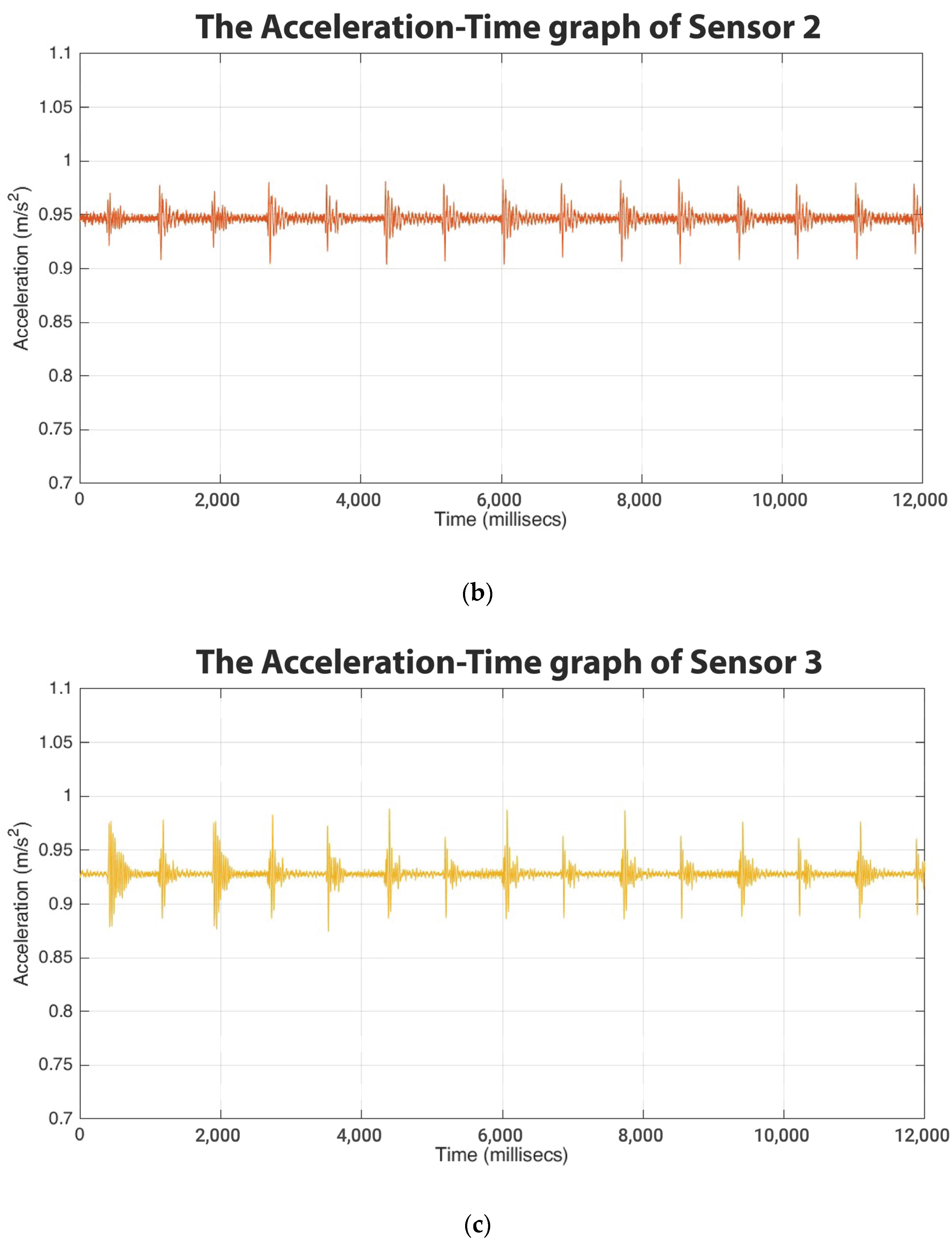
3. Results and Discussion
4. Conclusions
Author Contributions
Funding
Institutional Review Board Statement
Informed Consent Statement
Data Availability Statement
Conflicts of Interest
References
- Dilberoglu, U.M.; Gharehpapagh, B.; Yaman, U.; Dolen, M. The Role of Additive Manufacturing in the Era of Industry 4.0. Procedia Manuf. 2017, 11, 545–554. [Google Scholar] [CrossRef]
- Charalampous, P.; Kostavelis, I.; Tzovaras, D. Non-destructive quality control methods in additive manufacturing: A survey. Rapid Prototyp. J. 2020, 26, 777–790. [Google Scholar] [CrossRef]
- Wu, H.; Wang, Y.; Yu, Z. In situ monitoring of FDM machine condition via acoustic emission. Int. J. Adv. Manuf. Technol. 2016, 84, 1483–1495. [Google Scholar] [CrossRef]
- Wang, Y.; Xu, Z.; Wu, D.; Bai, J. Current status and prospects of polymer powder 3D printing technologies. Materials 2020, 13, 2406. [Google Scholar] [CrossRef]
- Gokhare, V.G.; Raut, D.N.; Shinde, D.K. A Review Paper on 3D-Printing Aspects and Various Processes Used in the 3D-Printing. Int. J. Eng. Res. Technol. 2017, 6, 953–958. Available online: https://www.researchgate.net/publication/350374850_A_Review_paper_on_3D-Printing_Aspects_and_Various_Processes_Used_in_the_3D-Printing (accessed on 10 January 2023).
- Dickinson, H. The Next Industrial Revolution? The Role of Public Administration in Supporting Government to Oversee 3D Printing Technologies. Public Adm. Rev. 2018, 78, 922–925. [Google Scholar] [CrossRef]
- Mehrpouya, M.; Dehghanghadikolaei, A.; Fotovvati, B.; Vosooghnia, A.; Emamian, S.S.; Gisario, A. The Potential of Additive Manufacturing in the Smart Factory Industrial 4.0: A Review. Appl. Sci. 2019, 9, 3865. [Google Scholar] [CrossRef]
- Jhodkar, D.; Nayak, A.; Gupta, K. Experimental investigation of nozzle clogging using vibration signal-based condition monitoring for fused deposition modeling. Mater. Sci. Forum 2021, 1037, 55–64. [Google Scholar] [CrossRef]
- In-Situ Monitoring and Diagnosing for Fused Filament Fabrication Process Ba: Discovery Service for Louisiana Tech University. Available online: https://eds.p.ebscohost.com/eds/pdfviewer/pdfviewer?vid=0&sid=7bc1c1a7-c160-4fc3-8644-4c6b2adbdc3e%40redis (accessed on 22 July 2022).
- Additive Manufacturing, Second Edition-Google Books. Available online: https://books.google.com/books?hl=en&lr=&id=70W4DwAAQBAJ&oi=fnd&pg=PP1&dq=additive+manufacturing&ots=lPr9AxEjOB&sig=nemKWzF_O2bZv9YUor3sAnfI8Js#v=onepage&q=additive%20manufacturing&f=false (accessed on 22 July 2022).
- Tlegenov, Y.; Hong, G.S.; Lu, W.F. Nozzle condition monitoring in 3D printing. Robot. Comput. Manuf. 2018, 54, 45–55. [Google Scholar] [CrossRef]
- Fu, Y.; Downey, A.; Yuan, L.; Pratt, A.; Balogun, Y. In situ monitoring for fused filament fabrication process: A review. Addit. Manuf. 2021, 38, 101749. [Google Scholar] [CrossRef]
- Rafiee, M.; Farahani, R.D.; Therriault, D. Multi-Material 3D and 4D Printing: A Survey. Adv. Sci. 2020, 7, 1902307. [Google Scholar] [CrossRef]
- Kantaros, A.; Ganetsos, T.; Piromalis, D. 3D and 4D Printing as Integrated Manufacturing Methods of Industry 4.0. Am. J. Eng. Appl. Sci. 2023, 16, 12–22. [Google Scholar] [CrossRef]
- Kalyan, B.P.; Kumar, L. 3D Printing: Applications in Tissue Engineering, Medical Devices, and Drug Delivery. AAPS PharmSciTech 2022, 23, 92. [Google Scholar] [CrossRef] [PubMed]
- Ali, H.; Issayev, G.; Shehab, E.; Sarfraz, S. A critical review of 3D printing and digital manufacturing in construction engineering. Rapid Prototyp. J. 2022, 28, 1312–1324. [Google Scholar] [CrossRef]
- Kantaros, A.; Ganetsos, T.; Petrescu, F.I.T. Three-Dimensional Printing and 3D Scanning: Emerging Technologies Exhibiting High Potential in the Field of Cultural Heritage. Appl. Sci. 2023, 13, 4777. [Google Scholar] [CrossRef]
- Gross, B.C.; Erkal, J.L.; Lockwood, S.Y.; Chen, C.; Spence, D.M. Evaluation of 3D printing and its potential impact on biotechnology and the chemical sciences. Anal. Chem. 2014, 86, 3240–3253. [Google Scholar] [CrossRef]
- Schubert, C.; Van Langeveld, M.C.; Donoso, L.A. Innovations in 3D printing: A 3D overview from optics to organs. Br. J. Ophthalmol. 2014, 98, 159–161. [Google Scholar] [CrossRef] [PubMed]
- Shahrubudin, N.; Lee, T.; Ramlan, R. An overview on 3D printing technology: Technological, materials, and applications. Procedia Manuf. 2019, 35, 1286–1296. [Google Scholar] [CrossRef]
- Mallakpour, S.; Tabesh, F.; Hussain, C.M. 3D and 4D printing: From innovation to evolution. Adv. Colloid Interface Sci. 2021, 294, 102482. [Google Scholar] [CrossRef]
- Puzatova, A.; Shakor, P.; Laghi, V.; Dmitrieva, M. Large-Scale 3D Printing for Construction Application by Means of Robotic Arm and Gantry 3D Printer: A Review. Buildings 2022, 12, 2023. [Google Scholar] [CrossRef]
- Guo, J.; Wu, J.; Sun, Z.; Long, J.; Zhang, S. Fault Diagnosis of Delta 3D Printers Using Transfer Support Vector Machine with Attitude Signals. IEEE Access 2019, 7, 40359–40368. [Google Scholar] [CrossRef]
- Li, C.; Cabrera, D.; Sancho, F.; Sánchez, R.-V.; Cerrada, M.; Long, J.; de Oliveira, J.V. Fusing convolutional generative adversarial encoders for 3D printer fault detection with only normal condition signals. Mech. Syst. Signal Process. 2021, 147, 107108. [Google Scholar] [CrossRef]
- Xu, Z.; Song, T.; Guo, S.; Peng, J.; Zeng, L.; Zhu, M. Robotics technologies aided for 3D printing in construction: A review. Int. J. Adv. Manuf. Technol. 2021, 118, 3559–3574. [Google Scholar] [CrossRef]
- Zhou, H.; Tawk, C.; Alici, G. A 3D Printed Soft Robotic Hand with Embedded Soft Sensors for Direct Transition Between Hand Gestures and Improved Grasping Quality and Diversity. IEEE Trans. Neural Syst. Rehabil. Eng. 2022, 30, 550–558. [Google Scholar] [CrossRef] [PubMed]
- Brunner, T.A.; Delley, M.; Denkel, C. Consumers’ attitudes and change of attitude toward 3D-printed food. Food Qual. Prefer. 2018, 68, 389–396. [Google Scholar] [CrossRef]
- Tejada-Ortigoza, V.; Cuan-Urquizo, E. Towards the Development of 3D-Printed Food: A Rheological and Mechanical Approach. Foods 2022, 11, 1191. [Google Scholar] [CrossRef]
- Ma, Y.; Zhang, L. Formulated food inks for extrusion-based 3D printing of personalized foods: A mini review. Curr. Opin. Food Sci. 2022, 44, 100803. [Google Scholar] [CrossRef]
- Li, Z.; Zhang, D.; Shao, L.; Han, S. Experimental investigation using vibration testing method to optimize feed parameters of color mixing nozzle for fused deposition modeling color 3D printer. Adv. Mech. Eng. 2019, 11, 1687814019896196. [Google Scholar] [CrossRef]
- Zhang, D.; Li, Z.; Qin, S.; Han, S. Optimization of vibration characteristics of Fused Deposition Modeling color 3D printer based on modal and power spectrum method. Appl. Sci. 2019, 9, 4154. [Google Scholar] [CrossRef]
- Gutiérrez, E.; Barreto, J.d.J.; Garcia-Hernandez, S.; Morales, R.; González-Solorzano, M.G. Decrease of nozzle clogging through fluid flow control. Metals 2020, 10, 1420. [Google Scholar] [CrossRef]
- Lee, A.; Sudau, K.; Ahn, K.H.; Lee, S.J.; Willenbacher, N. Optimization of experimental parameters to suppress nozzle clogging in inkjet printing. Ind. Eng. Chem. Res. 2012, 51, 13195–13204. [Google Scholar] [CrossRef]
- Barati, H.; Wu, M.; Kharicha, A.; Ludwig, A. A transient model for nozzle clogging. Powder Technol. 2018, 329, 181–198. [Google Scholar] [CrossRef]
- Tanveer, Q.; Mishra, G.; Mishra, S.; Sharma, R. Effect of infill pattern and infill density on mechanical behaviour of FDM 3D printed Parts- a current review. Mater. Today Proc. 2022, 62, 100–108. [Google Scholar] [CrossRef]
- Tao, Y.; Kong, F.; Li, Z.; Zhang, J.; Zhao, X.; Yin, Q.; Xing, D.; Li, P. A review on voids of 3D printed parts by fused filament fabrication. J. Mater. Res. Technol. 2021, 15, 4860–4879. [Google Scholar] [CrossRef]
- Jandyal, A.; Chaturvedi, I.; Wazir, I.; Raina, A.; Haq, M.I.U. 3D printing—A review of processes, materials and applications in industry 4.0. Sustain. Oper. Comput. 2022, 3, 33–42. [Google Scholar] [CrossRef]
- De Rosa, I.M.; Sarasini, F. Use of PVDF as acoustic emission sensor for in situ monitoring of mechanical behaviour of glass/epoxy laminates. Polym. Test. 2010, 29, 749–758. [Google Scholar] [CrossRef]
- Jackson, B.; Fouladi, K.; Eslami, B. Multi-Parameter Optimization of 3D Printing Condition for Enhanced Quality and Strength. Polymers 2022, 14, 1586. [Google Scholar] [CrossRef]
- Jadhav, A.; Jadhav, V.S. A review on 3D printing: An additive manufacturing technology. Mater. Today Proc. 2022, 62, 2094–2099. [Google Scholar] [CrossRef]
- Asutkar, S.; Korrapati, M.; Gupta, D.; Tallur, S. Novel Elastomer Vibration Sensor for Machine Health-Monitoring Applications. IEEE Sens. Lett. 2020, 4, 2501404. [Google Scholar] [CrossRef]
- IEEE Industrial Electronics Society; Xi’an li Gong Da Xue; IEEE Singapore Section. Industrial Electronics Chapter, and Institute of Electrical and Electronics Engineers. In Proceedings of the 14th IEEE Conference on Industrial Electronics and Applications (ICIEA 2019), Xi’an, China, 19–21 June 2019. [Google Scholar]
- He, K.; Yang, Z.; Bai, Y.; Long, J.; Li, C. Intelligent fault diagnosis of delta 3D printers using attitude sensors based on support vector machines. Sensors 2018, 18, 1298. [Google Scholar] [CrossRef]
- Rao, P.K.; Liu, J.; Roberson, D.; Kong, Z.; Williams, C. Online Real-Time Quality Monitoring in Additive Manufacturing Processes Using Heterogeneous Sensors. J. Manuf. Sci. Eng. 2015, 137, 061007. [Google Scholar] [CrossRef]
- Gomathi, K.; Ganesh, T.; Bharanidharan, J.; Prajathkar, A.A.; Aravinthan, R. Condition Monitoring of 3D Printer Using Micro Accelerometer. IOP Conf. Ser. Mater. Sci. Eng. 2021, 1055, 012035. [Google Scholar] [CrossRef]


| Printer Function | Nozzle Condition | Schematic of Nozzle Conditions | Extrusion Temp. | Bed Temp. | Print Speed |
|---|---|---|---|---|---|
| Normal | Unclogged |  | 195 °C | 60 °C | 60 mm/s |
| Limited | Slight clogging |  | 185 °C | 60 °C | 60 mm/s |
| Unacceptable | Partially clogged |  | 175 °C | 60 °C | 60 mm/s |
| Unacceptable | Completely clogged |  | 165 °C | 60 °C | 60 mm/s |
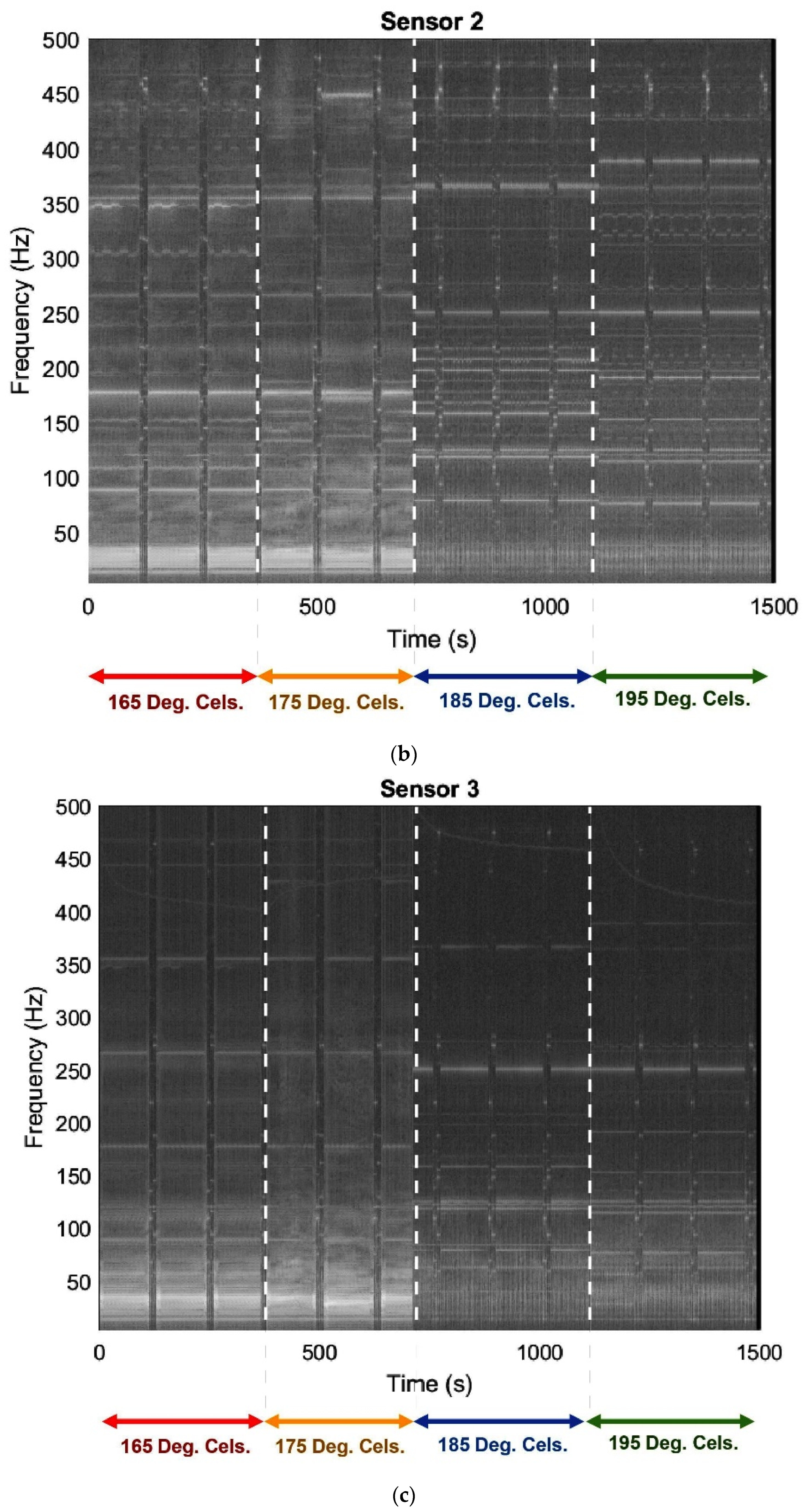
| Sensor | Observed Frequencies | |||
|---|---|---|---|---|
| Normal | Limited | Unacceptable | Unacceptable | |
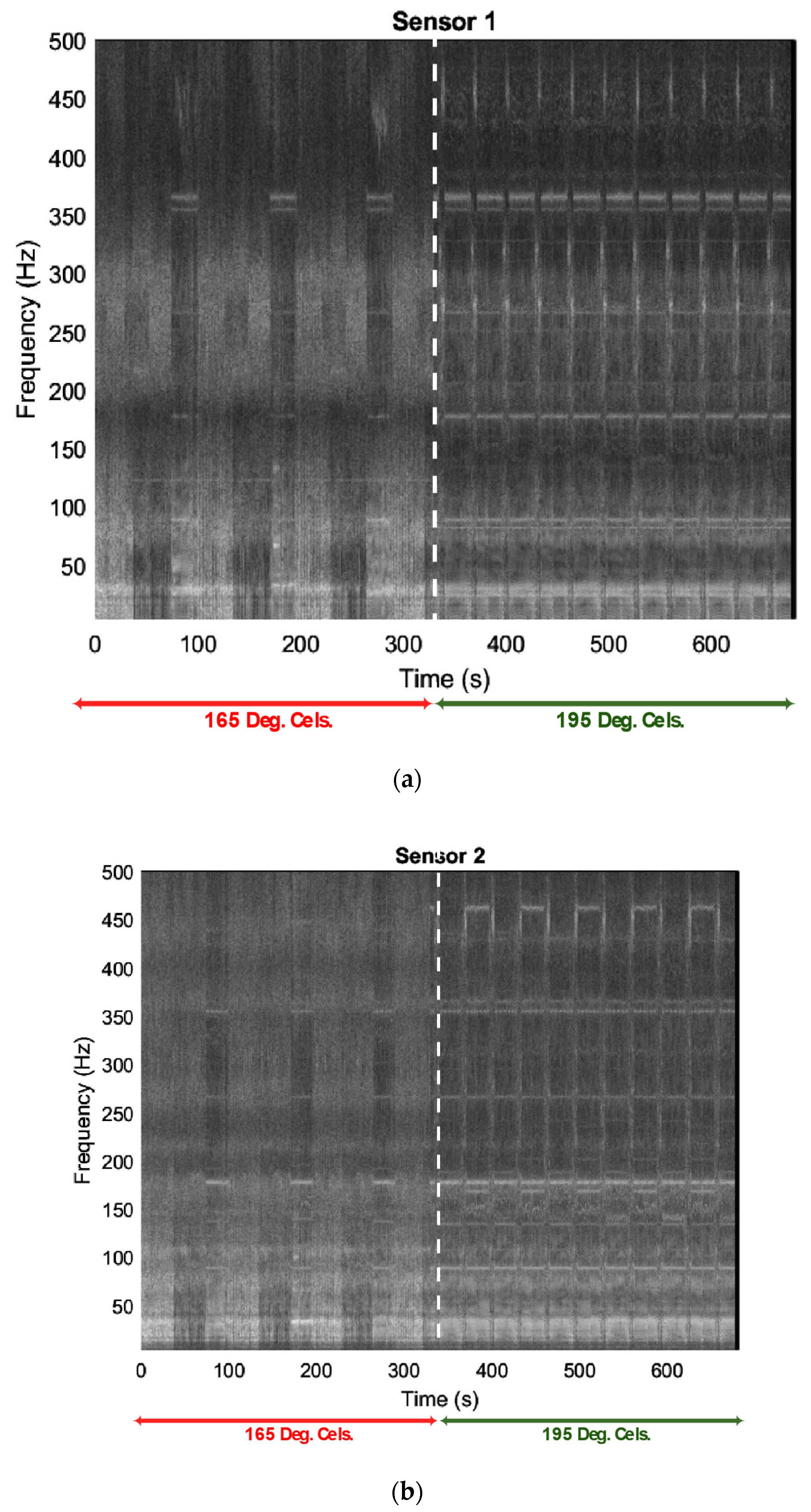
| Sensor 1 | 370 Hz, 270 Hz, 250 Hz | 370 Hz, 270 Hz, 250 Hz | 370 Hz, 350 Hz, 270 Hz, 180 Hz | 370 Hz, 350 Hz, 270 Hz, 180 Hz |
| Sensor 2 | 390 Hz, 370 Hz, 250 Hz, 200 Hz | 370 Hz, 250 Hz, 220 Hz, 200 Hz | 450 Hz, 350 Hz, 270 Hz, 180 Hz | 350 Hz, 270 Hz, 180 Hz |
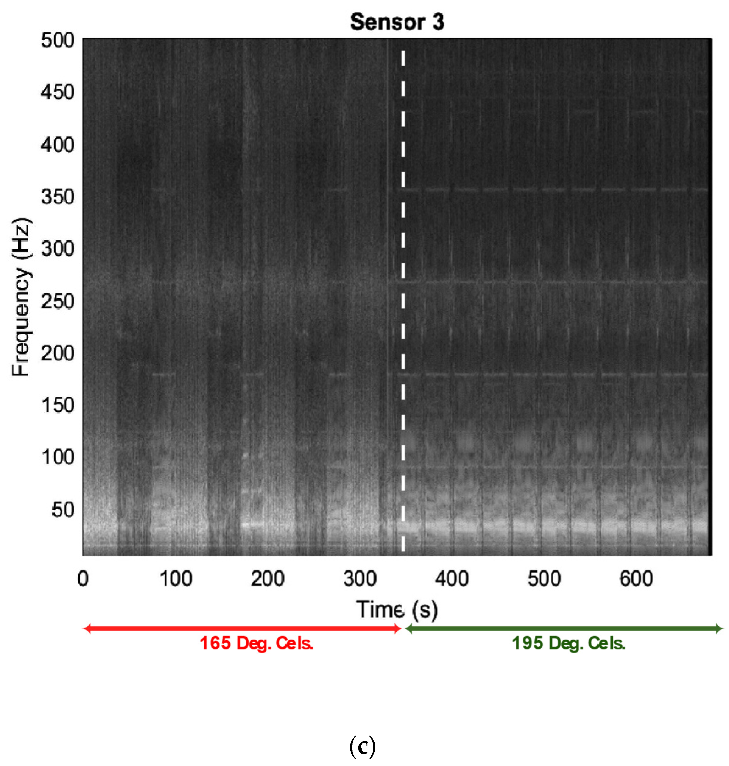
| Sensor 3 | 370 Hz, 250 Hz | 370 Hz, 250 Hz | 350 Hz, 270 Hz, 180 Hz | 350 Hz, 270 Hz, 180 Hz |
| Sensor | Observed Frequencies | |
|---|---|---|
| Normal | Unacceptable | |
| Sensor 1 | 370 Hz, 270 Hz, 180 Hz | Undiscovered |
| Sensor 2 | 370 Hz, 270 Hz, 180 Hz | Undiscovered |
| Sensor 3 | 370 Hz, 270 Hz, 180 Hz | Undiscovered |
Disclaimer/Publisher’s Note: The statements, opinions and data contained in all publications are solely those of the individual author(s) and contributor(s) and not of MDPI and/or the editor(s). MDPI and/or the editor(s) disclaim responsibility for any injury to people or property resulting from any ideas, methods, instructions or products referred to in the content. |
© 2023 by the authors. Licensee MDPI, Basel, Switzerland. This article is an open access article distributed under the terms and conditions of the Creative Commons Attribution (CC BY) license (https://creativecommons.org/licenses/by/4.0/).
Share and Cite
Isiani, A.; Weiss, L.; Bardaweel, H.; Nguyen, H.; Crittenden, K. Fault Detection in 3D Printing: A Study on Sensor Positioning and Vibrational Patterns. Sensors 2023, 23, 7524. https://doi.org/10.3390/s23177524
Isiani A, Weiss L, Bardaweel H, Nguyen H, Crittenden K. Fault Detection in 3D Printing: A Study on Sensor Positioning and Vibrational Patterns. Sensors. 2023; 23(17):7524. https://doi.org/10.3390/s23177524
Chicago/Turabian StyleIsiani, Alexander, Leland Weiss, Hamzeh Bardaweel, Hieu Nguyen, and Kelly Crittenden. 2023. "Fault Detection in 3D Printing: A Study on Sensor Positioning and Vibrational Patterns" Sensors 23, no. 17: 7524. https://doi.org/10.3390/s23177524
APA StyleIsiani, A., Weiss, L., Bardaweel, H., Nguyen, H., & Crittenden, K. (2023). Fault Detection in 3D Printing: A Study on Sensor Positioning and Vibrational Patterns. Sensors, 23(17), 7524. https://doi.org/10.3390/s23177524