

Viewpoint Planning for Range Sensors Using Feature Cluster Constrained Spaces for Robot Vision Systems

 , ,
, ,  , ,
, ,
Abstract
:1. Introduction
1.1. -spaces for Solving the Viewpoint Planning Problem
1.2. Related Work
1.2.1. Synthesis
1.2.2. Sampling-Based
1.3. Need for Action
- Multi-stage formulation: The complexity of the VPP can be subdivided into multiple subproblems. Simple and more efficient solutions can then be individually formulated for each subproblem.
- Model-based solution: Assuming that a priori information about viewpoint constraints (vision system, object, and task) is available, this knowledge should be used in the most effective and analytical manner. Furthermore, in this study, it is assumed that each viewpoint constraint should be spatially modeled in the special Euclidean (6D) aligned to a synthesis approach (see Section 1.2). This can be carried out by characterizing each constraint as a topological space, i.e., . If all viewpoint constraints can then be modeled as topological spaces and integrated together into s, the search for viable candidates can be reduced to the selection of a sensor pose within such spaces.
- Viewpoint planning strategy: Taking into account the modularization of the VPP and the characterization of s, a superordinated, holistic viewpoint planning strategy must be outlined for delivering a final selection of valid viewpoint candidates.
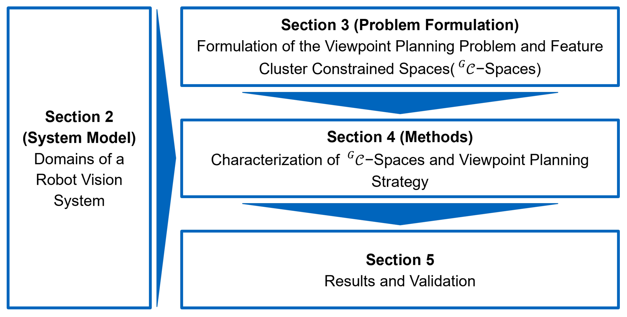
1.4. Outline
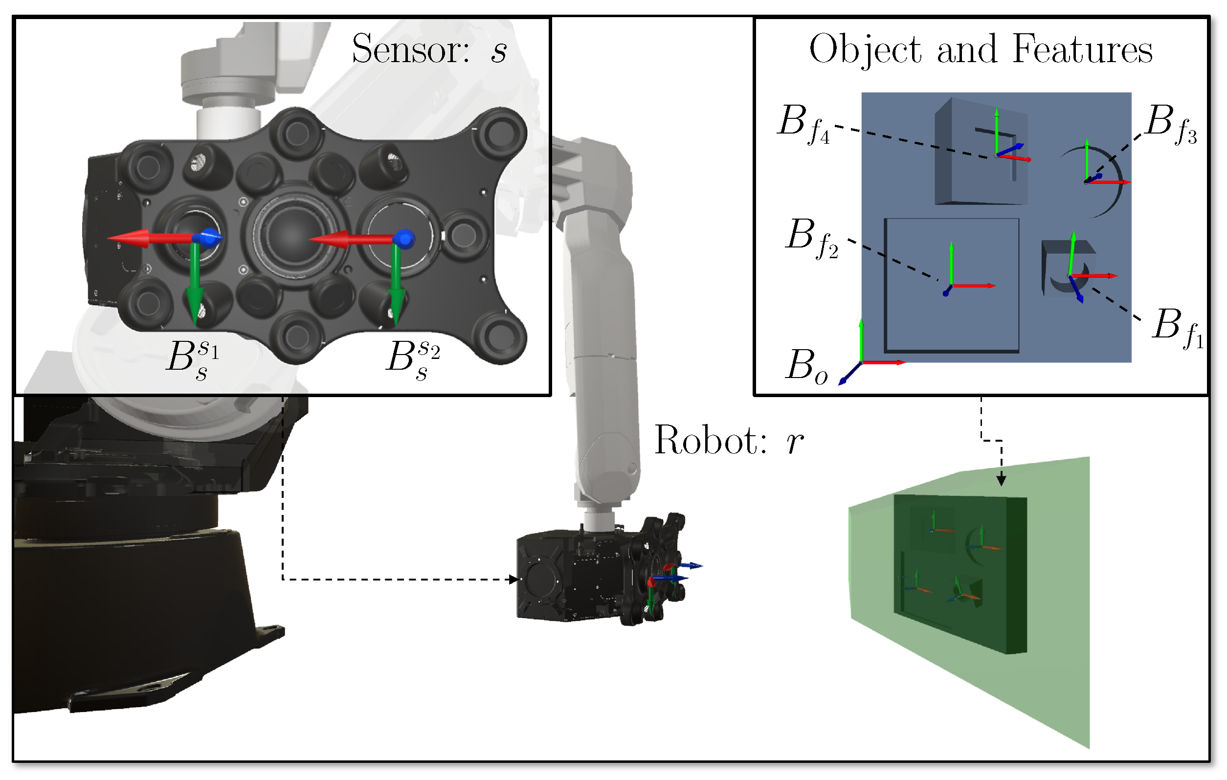
2. Robot Vision System Domains
2.1. Sensor
2.1.1. Frustum Space
2.1.2. Kinematics
2.1.3. Sensor Orientation
2.2. Object
2.3. Features
2.4. Robot
2.5. Viewpoint and Viewpoint Constraints
2.6. Vision Task
3. Formulation of the Viewpoint Planning Problem Based on s
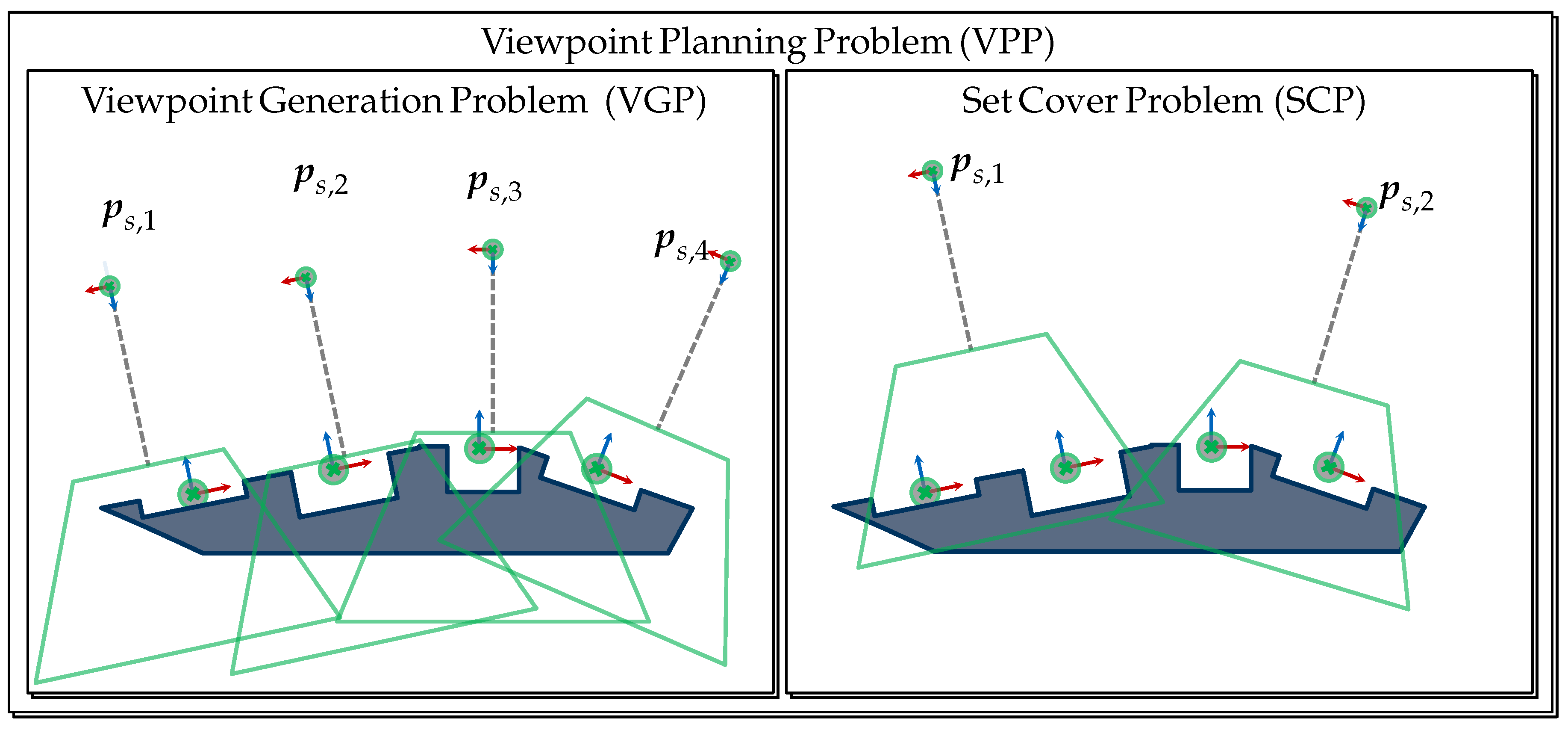
3.1. The Viewpoint Generation Problem
3.1.1. VGP with -spaces
3.1.2. VGP with -spaces
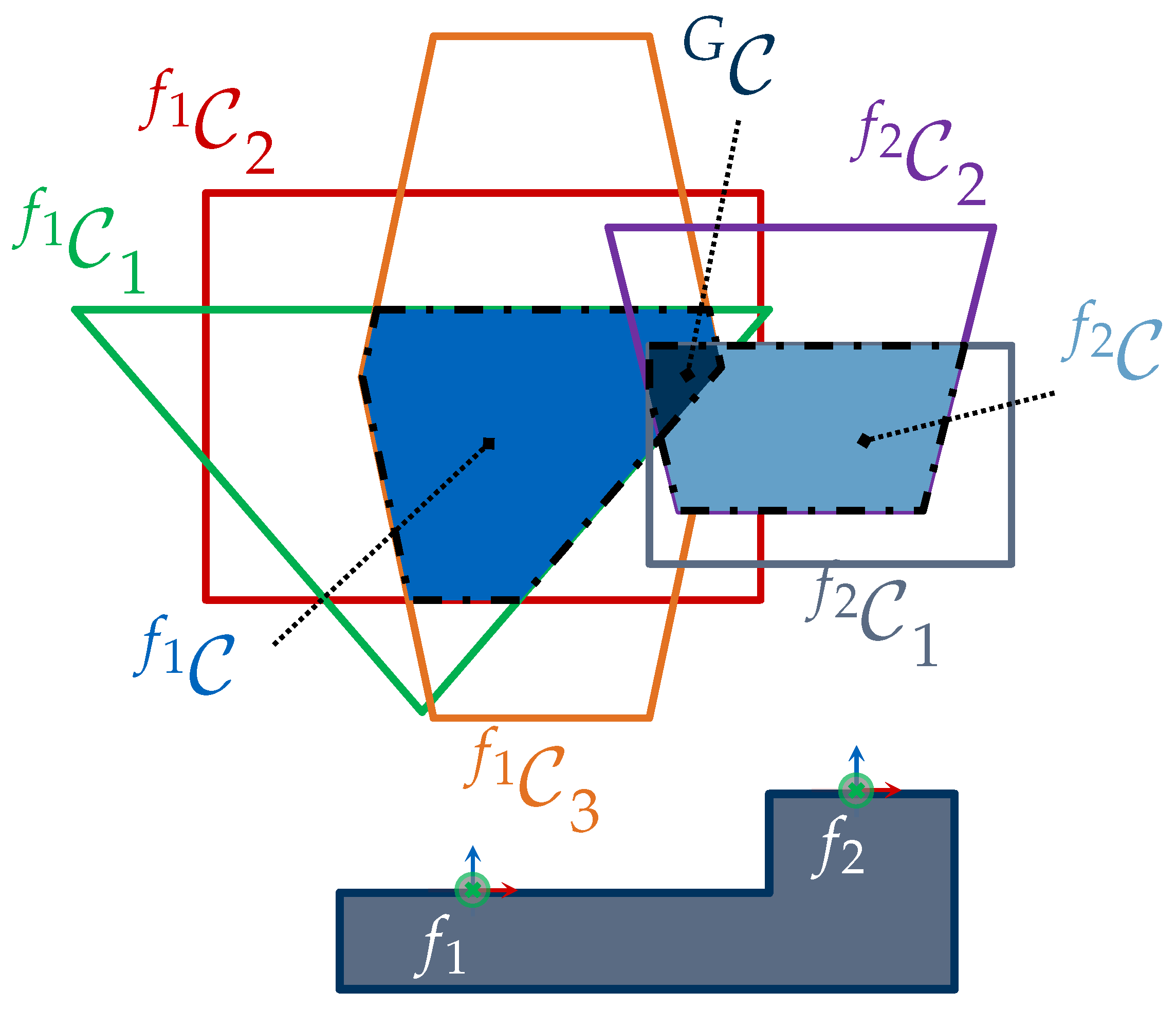
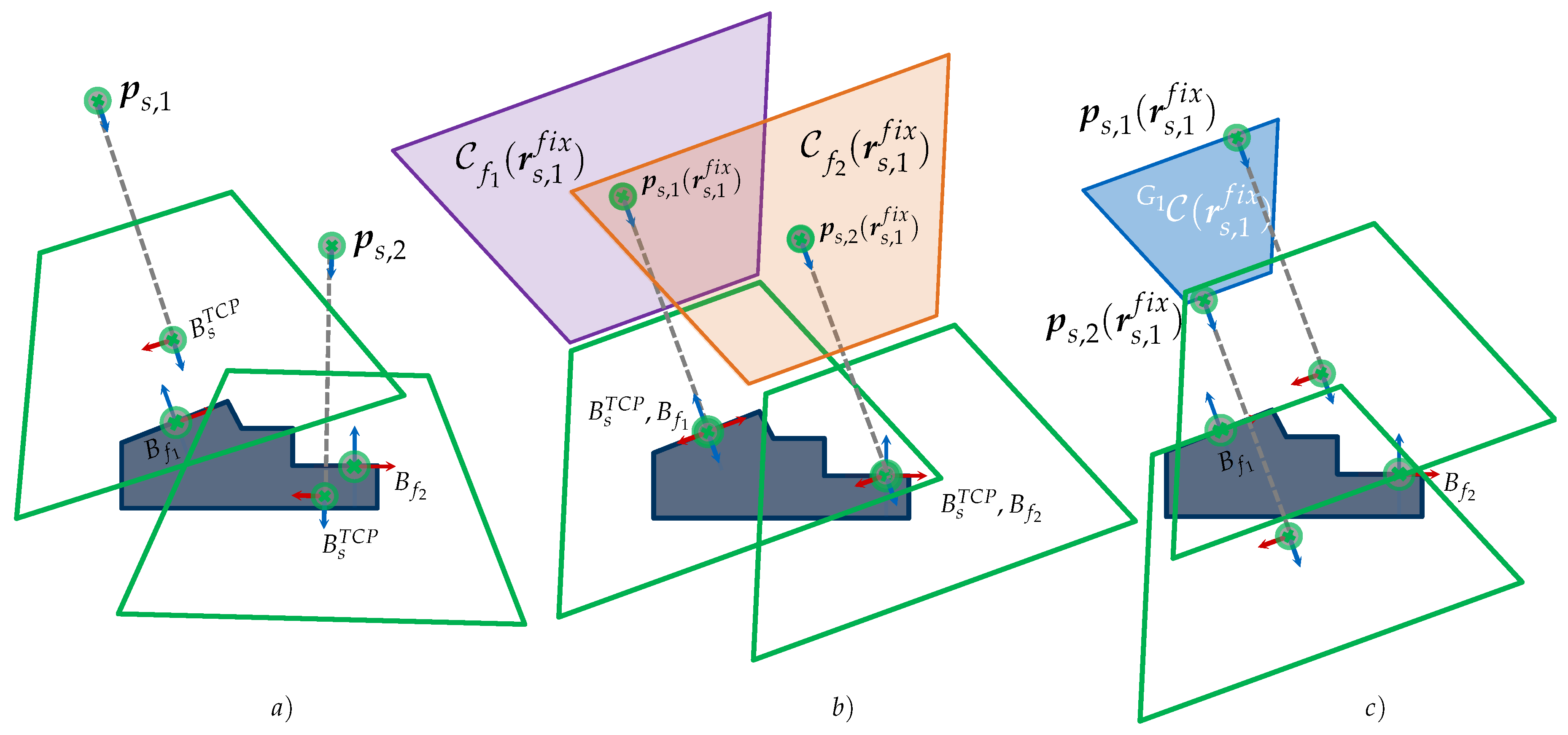
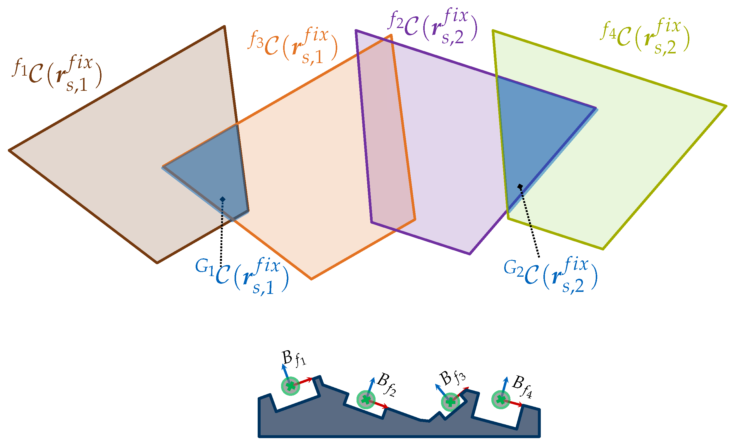
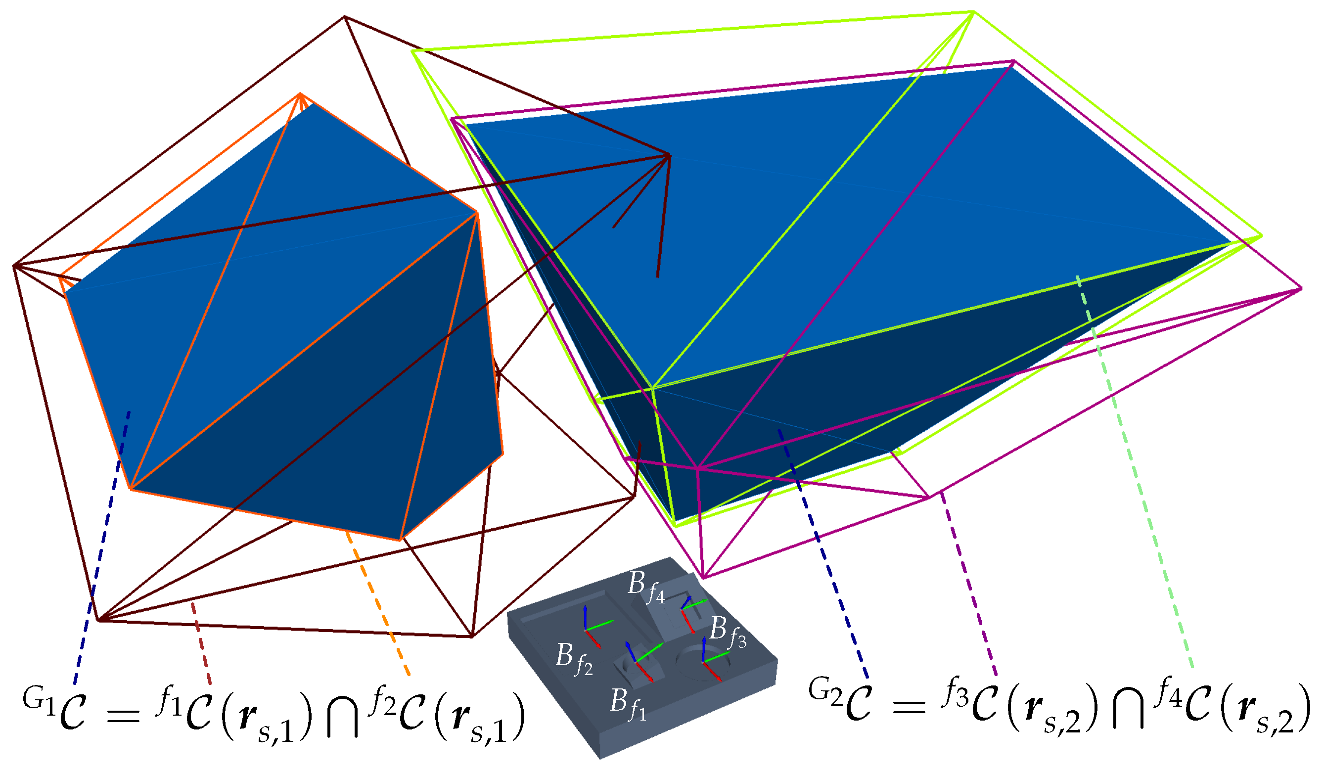
- The represents the intersection of all individual feature s as defined by Equation (6):
- If a -space is a non-empty manifold, i.e., ≠ Ø, there exists at least one sensor pose ∃ ∈ that fulfills all viewpoint constraints to acquire all features G.
3.2. The Set Cover Problem
3.2.1. Problem Formulation
3.2.2. Solving the SCP
3.3. Reformulation of the VPP
4. Methods
4.1. Feature Cluster Constrained Spaces
4.1.1. -spaces
| Algorithm 1 Characterization of the by reflection |
|
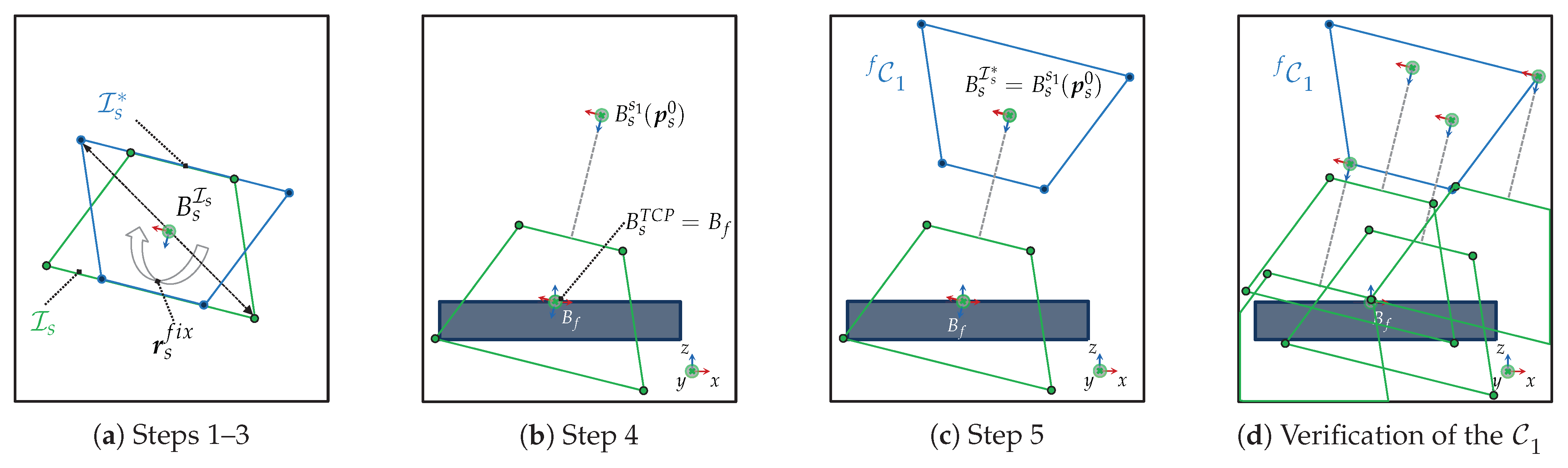
4.1.2. -spaces
- Fixed Sensor Orientation
- Characterization
- Verification
4.1.3. Summary
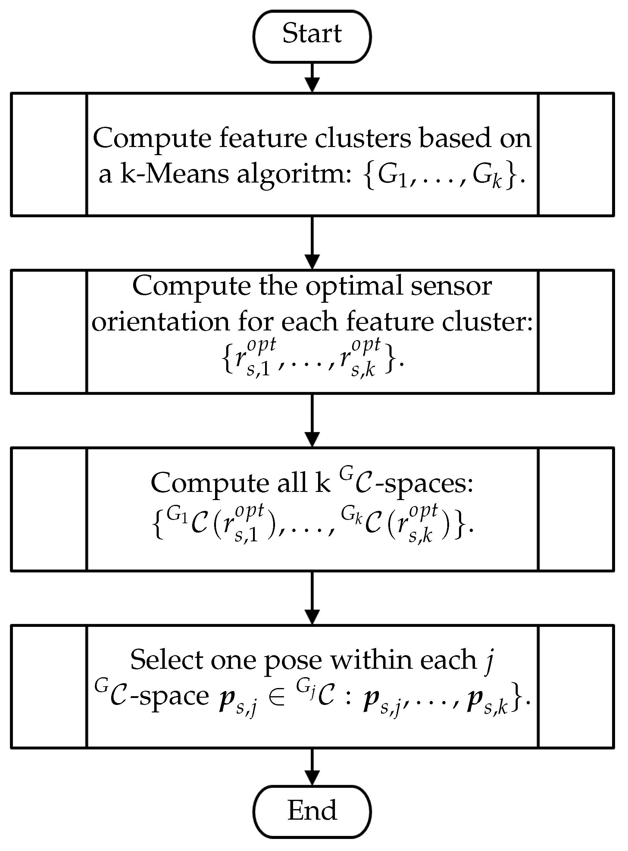
4.2. Viewpoint Planning Strategy
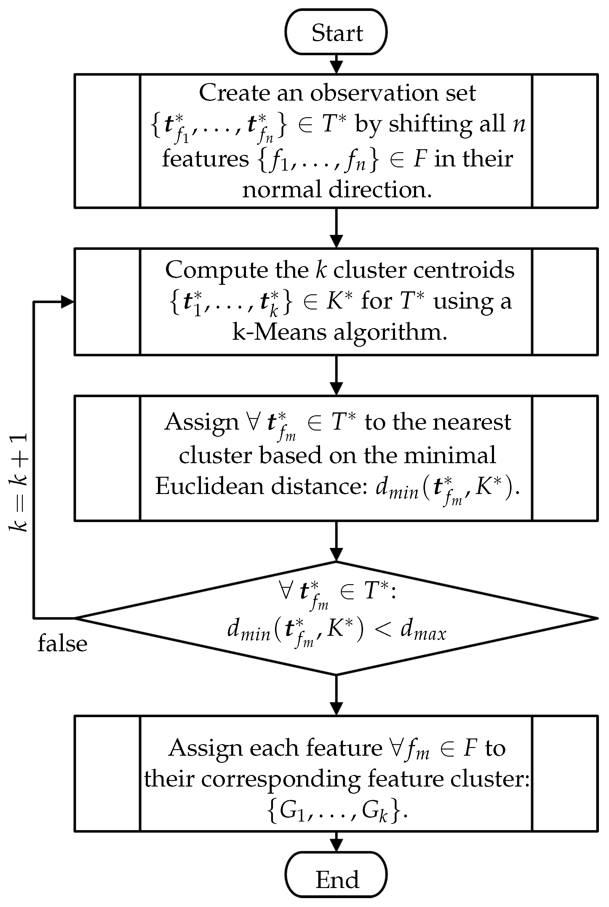
4.2.1. Feature Clusters
- Data Preparation
- Iteratively Clustering
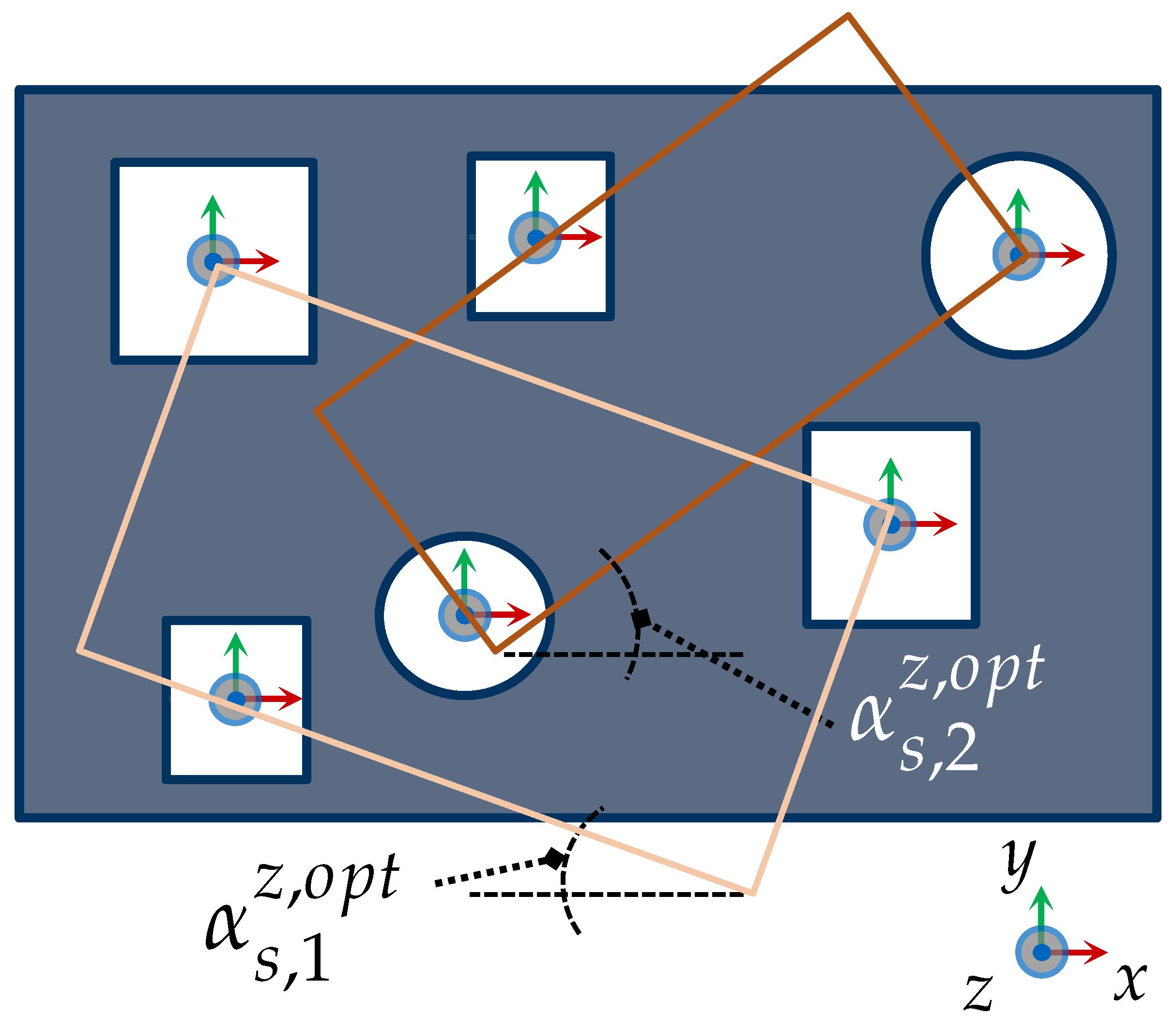
4.2.2. Sensor Orientation Optimization
- Formulation
- Incidence Angle
- Swing Angle
- Orientation of further imaging devices
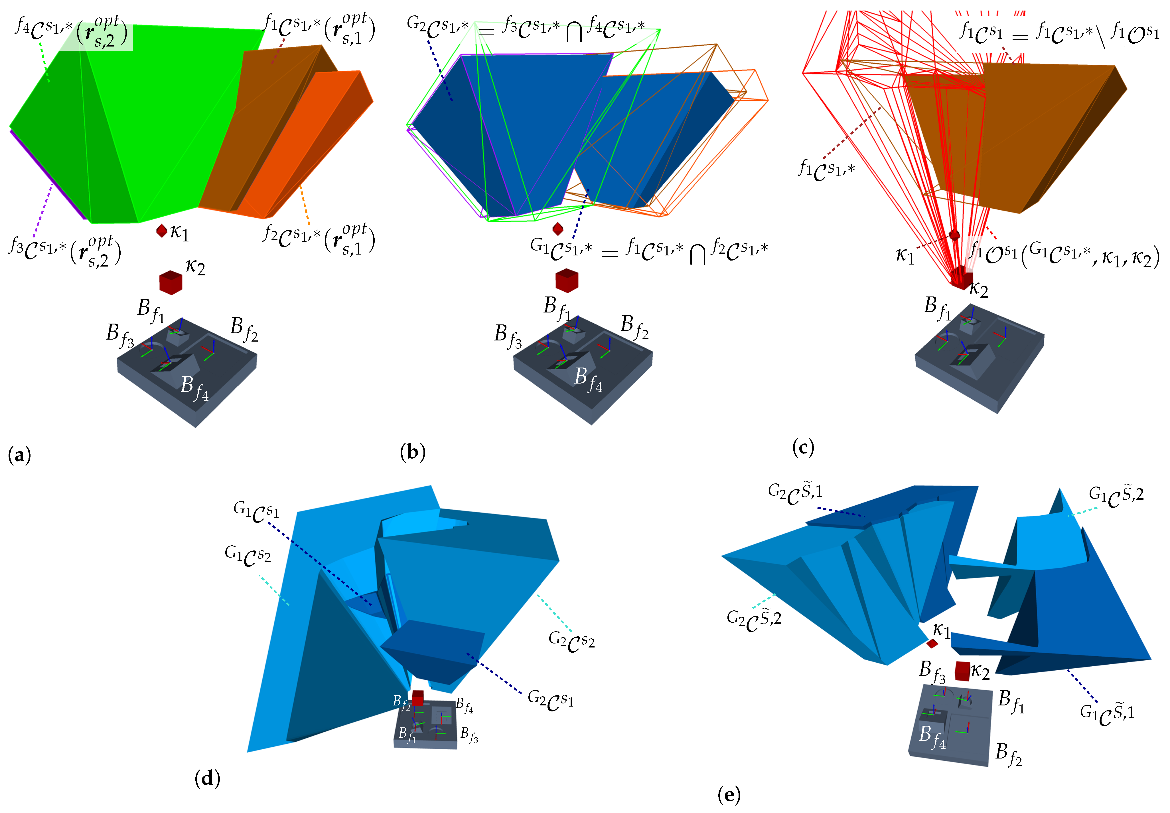
4.2.3. Computation of -spaces
- Integration Strategy of s
- Occlusion-Free s
- Strategy against invalid s
| Algorithm 2 Characterization of s based on s |
|
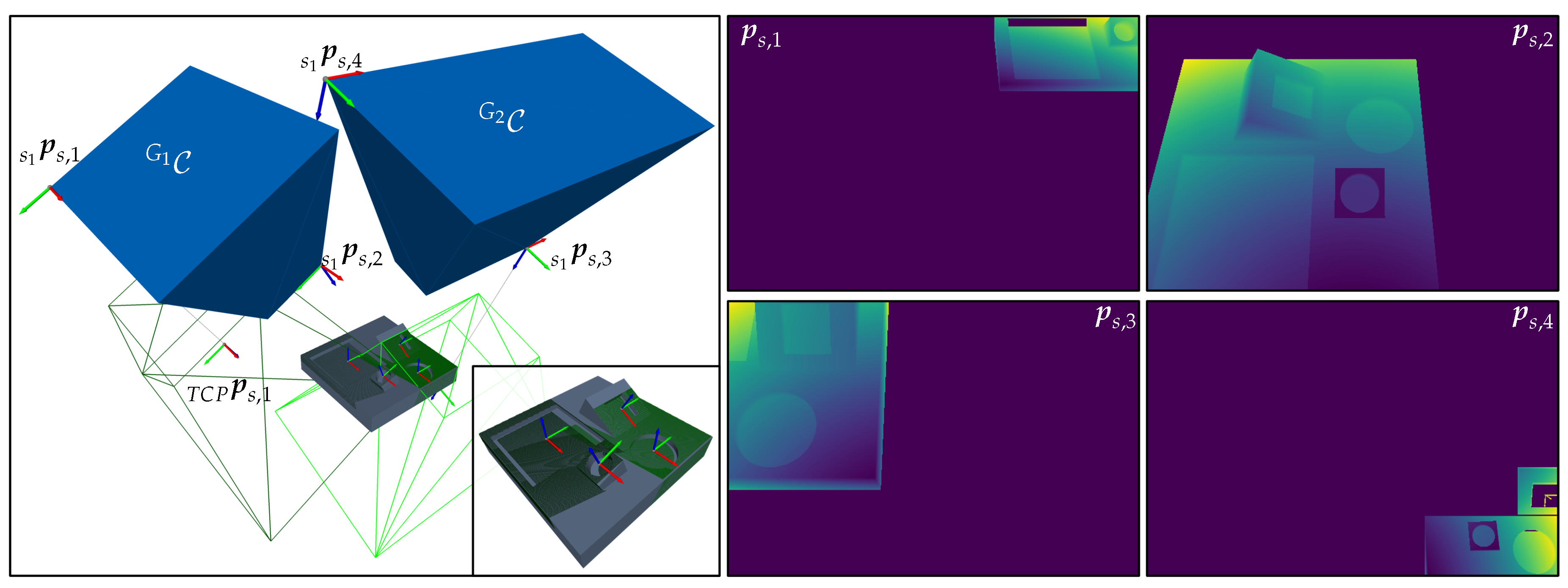
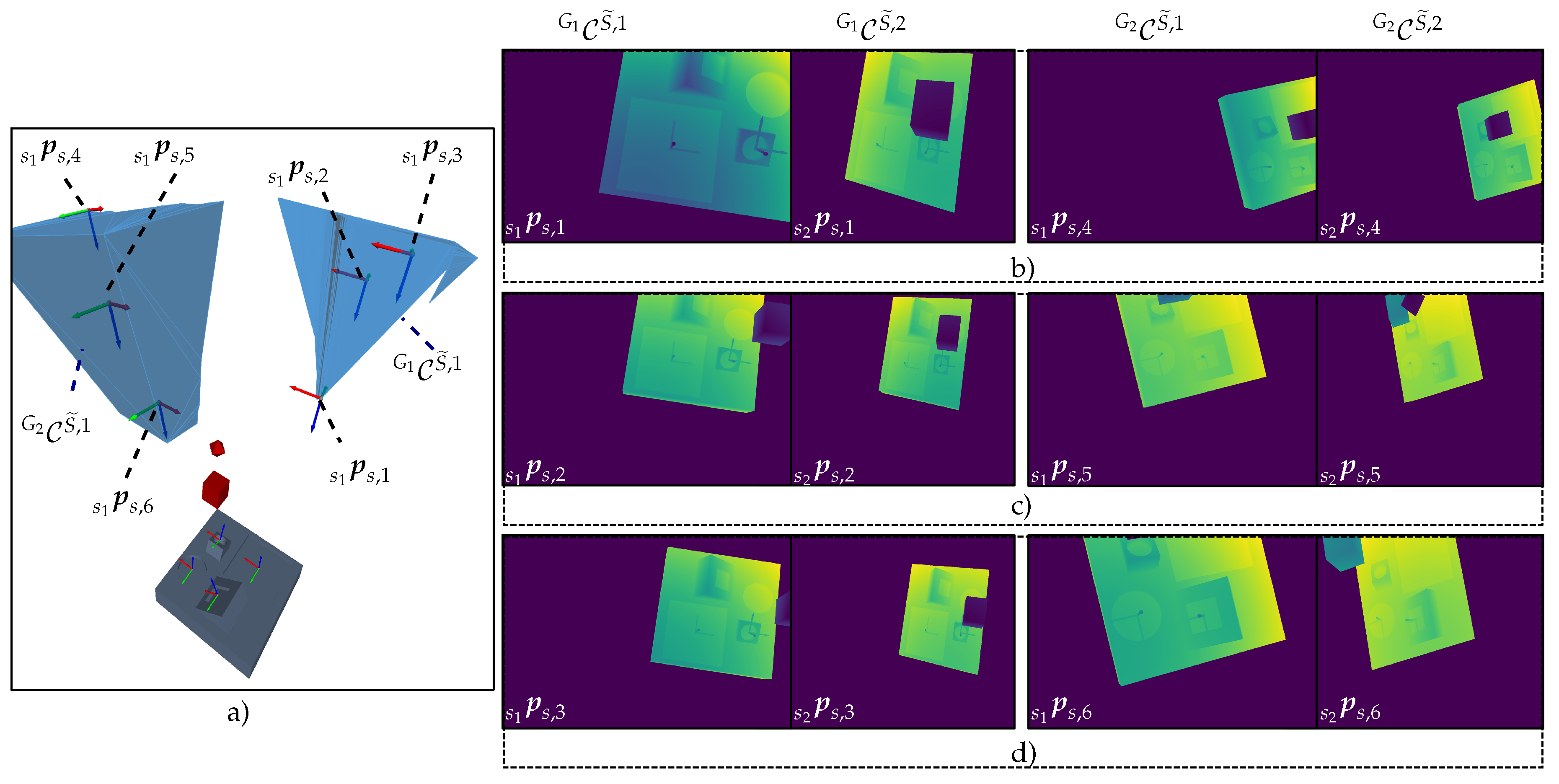
4.2.4. Sensor Pose Selection
4.3. Summary
5. Results
5.1. Robot Vision System with Structured Light Sensor
5.1.1. System Description
5.1.2. Vision Task Description
- Door Side: To evaluate the usability of the present framework in an industrial context, a car door was used as the probing object. Due to their topological complexity, feature density, and variability, car doors are well-known benchmark workpieces for evaluating metrology tasks and their automation.
- Number and Type of Features: The scalability was evaluated using inspection tasks with different numbers and types (points and circles) of features.
- Viewpoint Constraints: To analyze the efficacy and efficiency of the overall strategy, vision tasks with different viewpoint constraints were designed. All vision tasks regarded at least the most elementary viewpoint constraints – (i.e., the imaging characteristics of the sensor, feature geometry, and the consideration of kinematic errors). Moreover, for some vision tasks, a fourth viewpoint constraint was considered to ensure the satisfiability of the viewpoint constraints of the projector. Finally, for the vision tasks that included the viewpoint constraint , it was assumed that all features must have an occlusion-free visibility to the sensor and projector. Table 1 provides an overview of the considered viewpoint constraints.
5.1.3. Evaluation Metrics
- :
- The qualitative function assesses the following two conditions.
- A feature , including its entire geometry, must lie within the calculated frustum space of the corresponding sensor pose
- Both sensor and projector have free sight to the feature.
If both conditions are fulfilled, the feature is considered to be successfully acquired. - :
- The validity of each feature was further qualified based on the resulting 3D measurement, i.e., the point cloud. This metric counts the number of acquired points within a defined search radius around a feature. If there exist more points than a specified threshold, the feature can be considered to be valid.It needs to be noted that the proper evaluation of this condition requires that the measurements are perfectly aligned in the same coordinate system as the features and that the successful acquisition of surface points is guaranteed if all regarded constraints – are satisfied. Since our work neglects nonspatial constraints that may affect the quality of the measurement (e.g., exposure times or lighting conditions), the validity of the view plans was mainly assessed based on simulated measurements. The simulated measurements are generated by the proprietary software colin3D (Version 3.12) from ZEISS, which considers occlusion and maximal incidence angle constraints. Moreover, the measurements are perfectly aligned to the car door surface model.
- Computational Efficiency
- computation time for computing the necessary k feature clusters and corresponding optimized sensor orientations,
- computation time to characterize all individual s (one for each feature) considering the regarded viewpoint constraints,
- computation time to characterize all k s,
- total computation time of the vision task, corresponds to the sum of the times mentioned above.
5.1.4. Implementation
5.1.5. Results
- Measurability
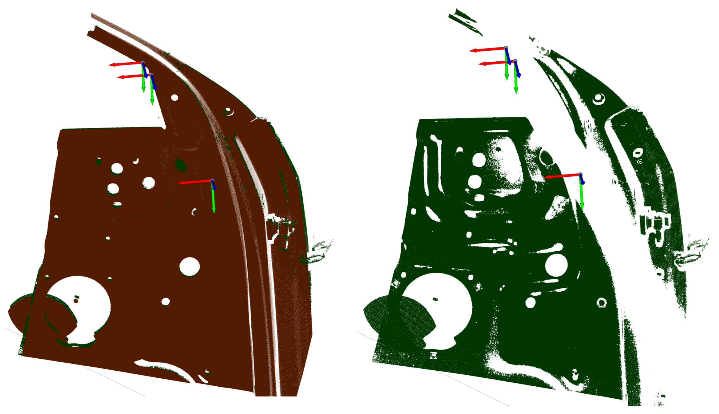
- Occlusion: All failed qualitative evaluations and the decrease in the measurability score if occlusion constraints were regarded can be attributed to the nonexistence of an occlusion-free space for the computed s with the chosen sensor orientation. The strategy proposed in Section 4.2.3 did not explicitly contemplate such cases. However, this problem could be straightforwardly solved by considering an alternative sensor orientation in the 7th step of Algorithm 2 when the intersection of consecutive s yields a non-empty manifold. Formulating such a strategy requires a more comprehensive analysis of the occlusion space, which falls outside the scope of this work.Furthermore, the failed evaluation of most features lying on the inside of the door was occasioned by occlusion with the door itself, which was initially neglected as an occluding object. However, an empirical analysis of some failed viewpoints showed that a positive evaluation could be achieved by recomputing the s of the affected features considering the car door as an occluding object, as seen in Figure 19.
- Missing points and misalignment: The quantitative evaluation of some individual viewpoints showed discrepancies between the simulation and the real measurements. These differences can be easily explained considering the requirements of the quantitative evaluation strategy proposed in Section 5.1.3 based on the acquisition of surface points. Due to the high reflectivity of the car door material and the fact that the optimization of the exposure time was neglected during the experiments, the acquisition of enough surface points in some areas could not be achieved, see Figure 20. On the other hand, a detailed evaluation of some failed viewpoints showed that the measurements could not be aligned correctly in other cases, causing a false-positive evaluation of some features. By manually optimizing the number of exposure times and individual values, more dense and better-aligned measurements could be obtained, mitigating most of the mentioned errors.
- Computational Efficiency
- It can be observed that the feature clustering and optimization of the sensor orientation can be regarded as the most efficient step of the strategy and represent, on average, less than 10% of the whole planning process. The experiments show the efficiency of the k-Means algorithm for such tasks, agreeing with the previous findings from [28].
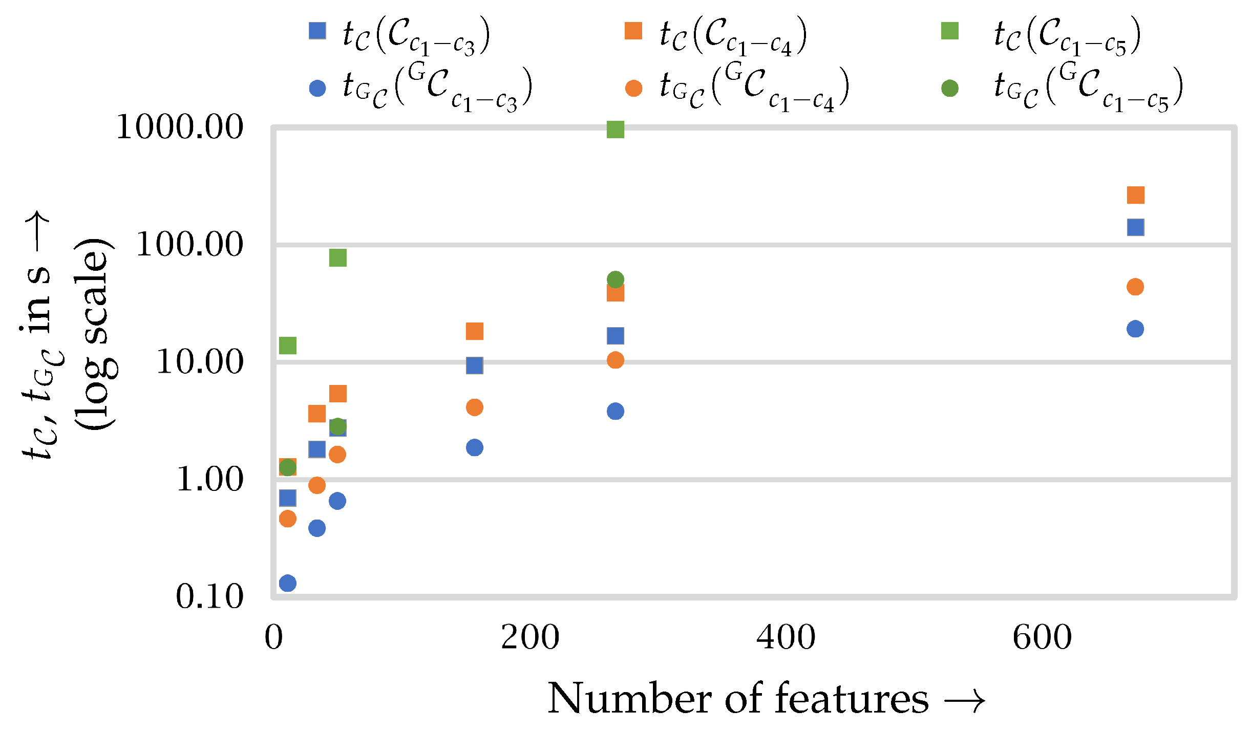
- The vision tasks that only incorporate the fundamental constraints – showed a high computational efficiency. These results were to be expected, taking into account that the characterization of these viewpoint constraints consists mainly of linear operations. This trend can be observed in Figure A2, showing the proportional increase between the computation time for the required s and the total number of features. This behavior can be further observed when the fourth constraint is considered. In this case, each must be spanned for each imaging device (sensor and projector), increasing the computation by a factor of two. On the other hand, taking into account the occlusion constraint considerably increased the computational complexity of the task. This behavior is also comprehensible, recalling that the characterization of occlusion-free s relies on ray-casting, which is well known to be a computationally expensive process.Moreover, neglecting occlusion constraints, the average computation time for the characterization of one was estimated at 60 ms. It needs to be noted that this time estimation includes a non-negligible computational overhead of all required operations, such as frame transformation operations using ROS-Services. In [4] the computation of a single was estimated, on average, at 4 ms.
- The computation of the s using intersecting Boolean operations proved to be highly efficient, requiring 10–15% of the total planning time. The experiments also confirm that the time effort increases with the number of intersecting spaces. However, by applying manifold decimation techniques after each Boolean intersection (cf. Section 4.2.3), the time effort could be considerably reduced. For instance, within the first vision task, the characterization of a with six s required 0.6 s, while the intersection of a with 44 s took 2.4 s. Furthermore, the computation times of the s considering occlusion constraints visualized in Figure A2 confirm that the intersection of more complex manifolds was, on average, more time-consuming.
- Determinism
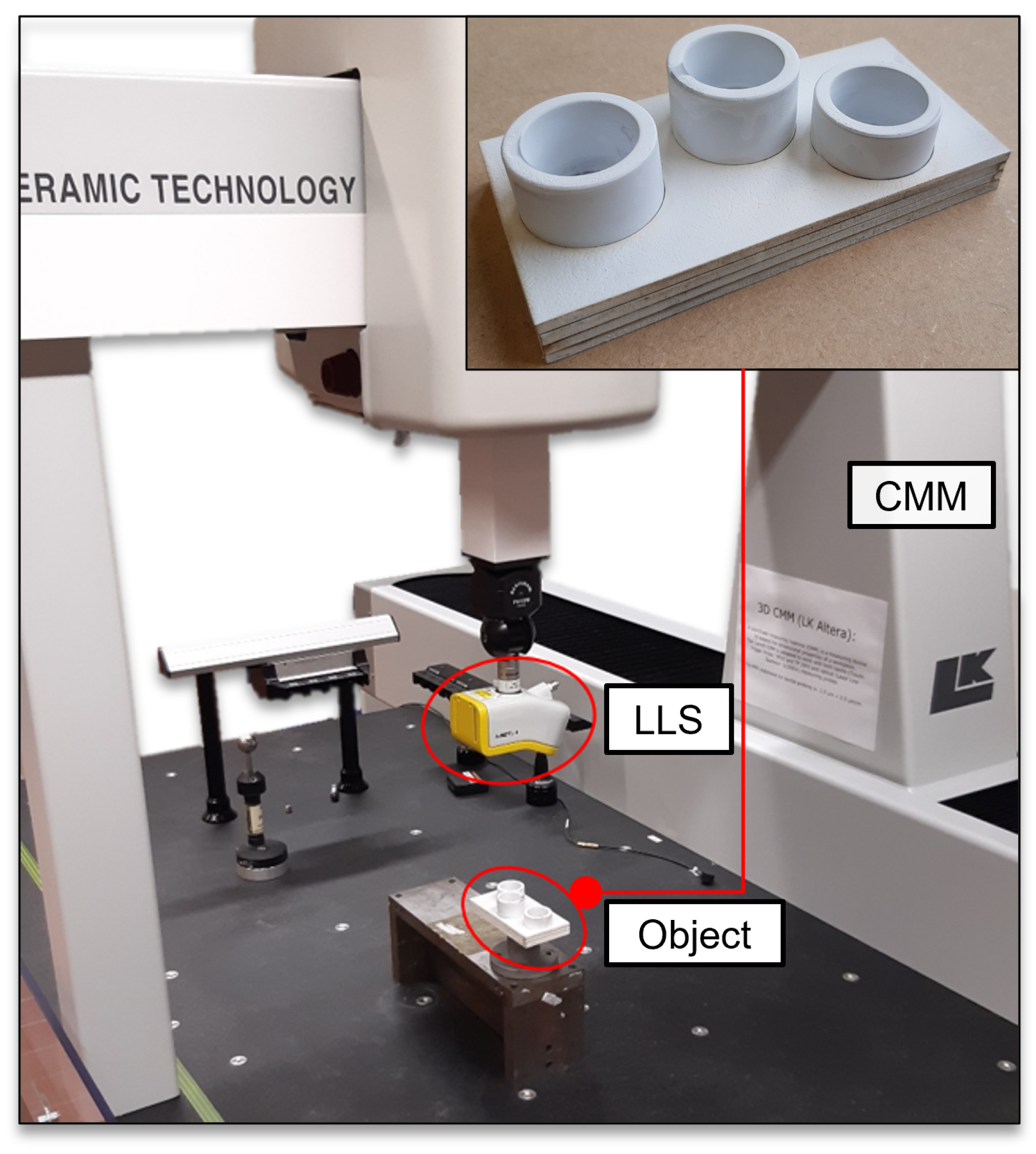
5.2. CMM with Laser Line Scanner
5.2.1. System Description
5.2.2. Vision Task Description
5.2.3. Assumptions and Adaptation of the Domain Models and Viewpoint Planning Strategy
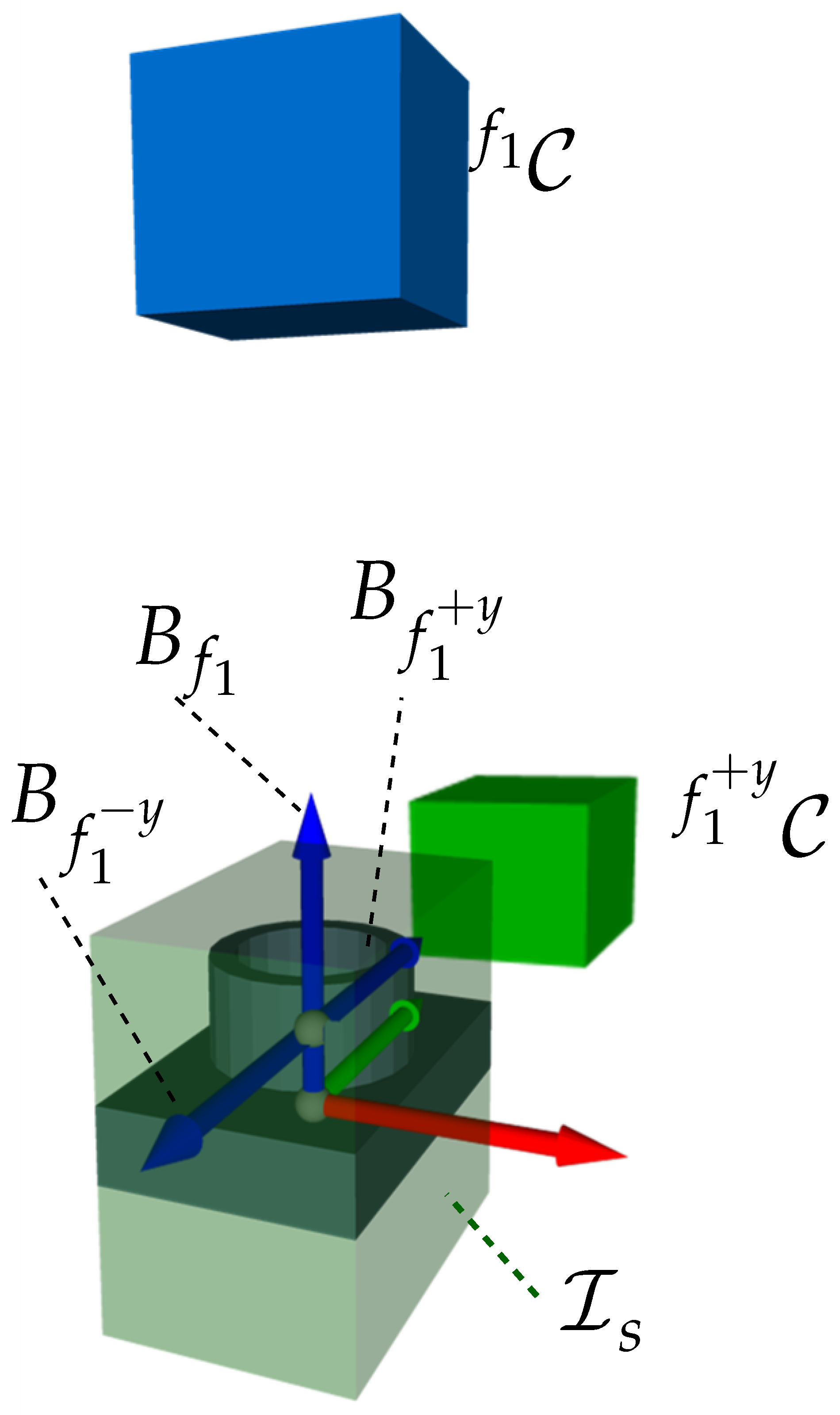
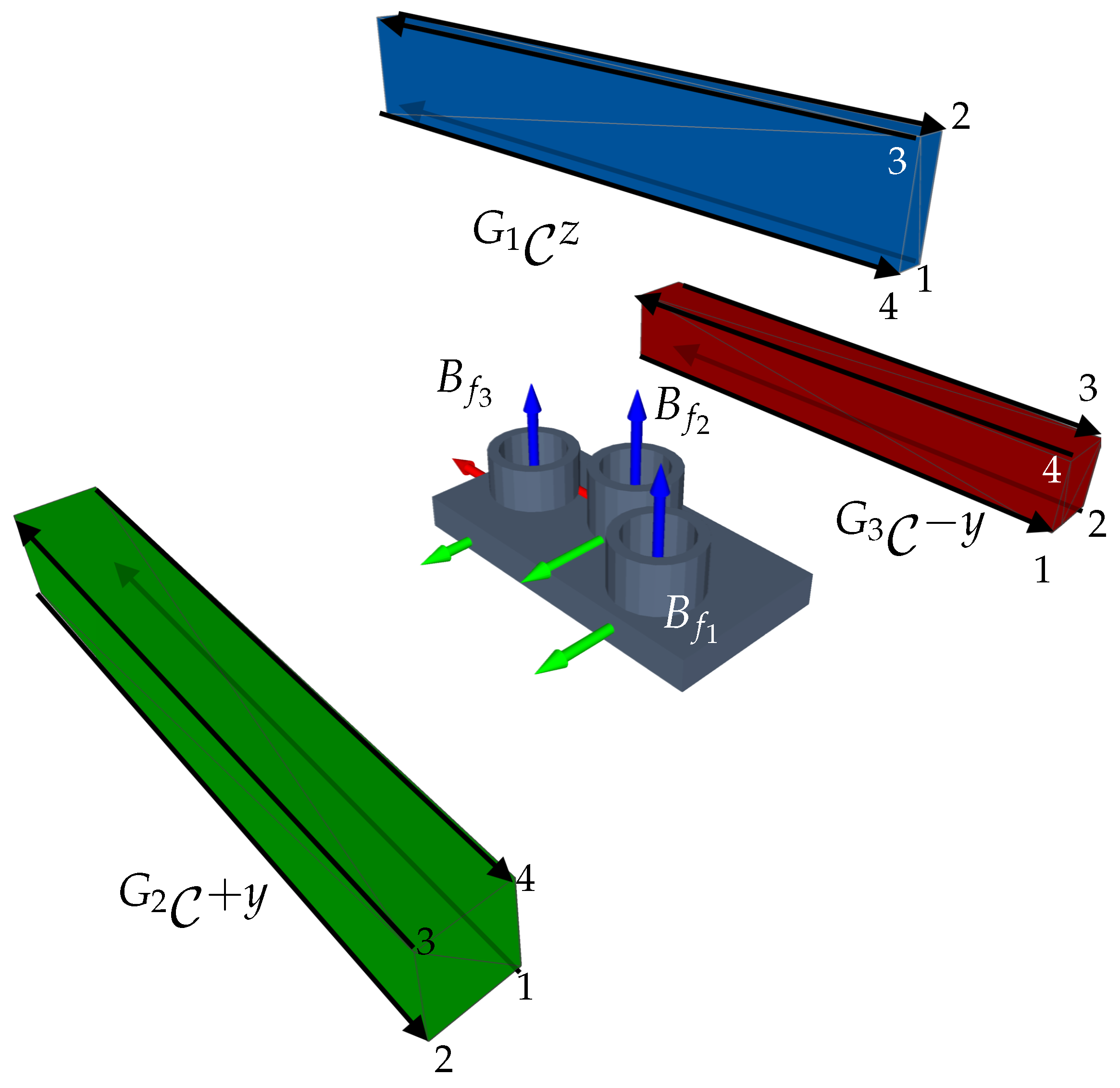
- Features: The measuring object comprises three cylinders with different positions (see Table A6). The feature frame of the cylinders is placed at the bottom. Taking into account the feature model from Section 2.3, which only considers one frame per feature and assumes that the whole cylinder can be acquired with a single measurement, the definition of the feature model must be extended to guarantee the acquisition of the cylinder’s surface area. Thus, two further features for each cylinder (, ) were introduced. The new feature frames are located at the half-height of the cylinder and their normal vectors (z-axis) are perpendicular to the x-axis of the feature’s origin. The geometrical length of these extra features corresponds to the height of the cylinders. An overview of the frames of all features corresponding to one cylinder are shown in Figure 22.
- Sensors and Acquisition of Surface Points: It is assumed that the LLS only moves in a straight line in the CMM’s workspace with a fixed sensor orientation. For this reason, we assume that all feature surface points can be acquired with a single scanning trajectory as long as the incidence angle constraint between the surface points and the sensor holds.
- and : Recalling that s are built based on the 3D sensor’s , we first considered a modification of the LLS’s 2D frustum. Recalling the previous assumption regarding the acquisition of surface points, let the LLS span a 3D composed of the 2D and a width corresponding to the distance of the scanning trajectory. The resulting of one scanning direction and the resulting s for one cylinder and its three features are visualized in Figure 22. Having characterized a 3D frustum, the approach presented in Algorithm 1 can be directly applied to span the required for one feature. The successful acquisition of one feature results from moving the sensor from an arbitrary viewpoint from one end of the to another arbitrary viewpoint at its other end. This study only considers the characterization of one for the sensor’s laser.
- and Multi-features: Within multi-feature scenarios, it is desirable to acquire as many features as possible during one linear motion. Therefore, in the simplest scenario, the length of all scanning trajectories corresponds to the size of the object’s longest dimension. Under this premise, we assume that the width of the , hence, of each single , corresponds to this exact length.
- Viewpoint Constraints: Equally to other vision systems, the successful acquisition of surface points depends on the compliance of some geometric viewpoint constraints, such as the imaging capabilities of the LLS () and the consideration of the features’ geometrical dimensions (). Since the scope of this study prioritizes the transferability of the viewpoint strategy, only these constraints were considered to guarantee the successful acquisition of the regarded features. The adaptation and validation of further viewpoint constraints lie outside the scope of this publication and remain to be further investigated.
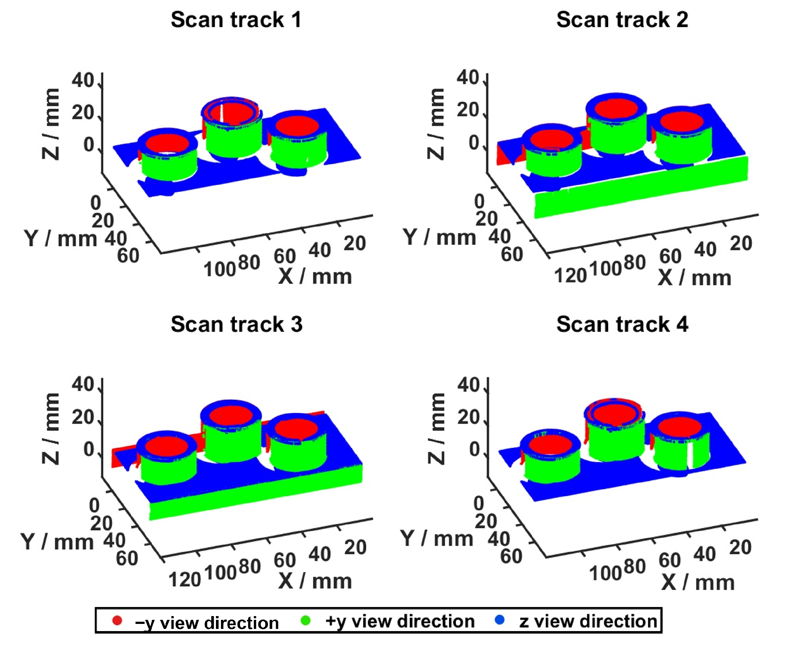
5.2.4. Results
5.3. Discussion
5.3.1. Efficacy
5.3.2. Computational Efficiency
5.3.3. Transferability
6. Conclusions
6.1. Summary
- Mathematical and generic formulation of the VPP to ease the transferability and promote the extensibility of the framework for diverse vision systems and tasks.
- Synthesis of s built upon s, inheriting some of their intrinsic advantages:
- -
- analytical, model-based, and closed-form solutions,
- -
- simple characterization based on constructive solid geometry () Boolean techniques,
- -
- infinite solutions for the seamless compensation of model uncertainties.
- Generic and modular viewpoint planning strategy, which can be adapted to diverse vision tasks, systems, and constraints.
6.2. Limitations and Future Work
Supplementary Materials
Author Contributions
Funding
Institutional Review Board Statement
Informed Consent Statement
Data Availability Statement
Acknowledgments
Conflicts of Interest
Abbreviations
| Feature-based constrained space | |
| Feature cluster constrained space | |
| RVS | Robot vision system |
| SCP | Set cover problem |
| VGP | Viewpoint generation problem |
| VPP | Viewpoint planning problem |
Appendix A. Tables and Figures

| Viewpoint Constraint | Brief Description |
|---|---|
| 1. Frustum Space | The most restrictive and fundamental constraint is given by the imaging capabilities of the sensor. This constraint is fulfilled in its most elementary formulation if at least the feature’s origin lies within the frustum space (cf. Section 2.1.1). |
| 2. Feature Orientation and Incidence Angle | The maximal permitted incidence angle between the optical axis and the feature normal is not allowed to exceed a maximal angle determined by the sensor manufacturer. (2). |
| 3. Feature Geometry | This constraint can be considered an extension of the first viewpoint constraint and is fulfilled if all surface points of a feature can be acquired by a single viewpoint, hence, lying within the image space. |
| 4. Kinematic Error | Within the context of real applications, model uncertainties affecting the nominal sensor pose compromise a viewpoint’s validity. Hence, any factor, e.g., kinematic alignment, robot’s pose accuracy, affecting the overall kinematic chain of the RVS must be considered. |
| 5. Sensor Accuracy | It is assumed that the sensor accuracy may vary within the sensor image space. |
| 6. Feature Occlusion | A viewpoint can be considered valid if a free line of sight exists from the sensor to the feature. |
| 7. Bistatic Sensor and Multisensor | Recalling the bistatic nature of range sensors, all viewpoint constraints must be valid for all lenses or active sources. |
| Notation | Index Description |
|---|---|
| x :=variable, parameter, vector, frame or transformation | |
| d :=RVS domain, i.e., sensor, robot, feature, object, environment or d element of a list or set | |
| n :=related domain, additional notation or depending variable | |
| r :=base frame of the coordinate system or space of feature f | |
| b :=origin frame of the coordinate system | |
| Notes | The indexes r and b only apply for pose vectors, frames, and transformations. |
| Example | |
|
| Feature | ||||||
|---|---|---|---|---|---|---|
| Topology | Circle | Slot | Circle | Slot | Octahedron | Cube |
| Dimensions in mm | radius | length = 150 | radius | length = 50 | edge length | length = |
| Translation vector in object’s frame in mm | ||||||
| Rotation in Euler Angles in object’s frame in |
| Range Sensor | 1 | 2 | |
|---|---|---|---|
| Manufacturer | Carl Zeiss Optotechnik GmbH | Nikon | |
| Model | COMET Pro AE | LC60Dx | |
| 3D Acquisition Method | Digital Fringe Projection | Laser Scanner | |
| Imaging Devices | Monochrome Camera () | Blue Light LED-Fringe Projector () | Laser Diode and Optical Sensor |
| FOV angles | , | , | |
| Working distances and corresponding near, middle, and far planes. | |||
| Vision Tasks Configuration | Results | |||||||||||
|---|---|---|---|---|---|---|---|---|---|---|---|---|
| Vision Task | Door Side | Feature Type | Constraints | Nr. of Features | Nr. of Clusters | Measurability Index in %, | Computation Time in s | |||||
| 1 | All | All | 1–3 | 673 | 75 | 97.77 | 8.35 | 140.94 | 19.11 | 168.41 | ||
| 2 | All | All | 1–4 | 673 | 77 | 97.47 | 9.28 | 265.99 | 43.59 | 318.86 | ||
| 3 | All | Circles | 1–3 | 50 | 12 | 92.00 | 1.53 | 2.76 | 0.66 | 4.94 | ||
| 4 * | All | Circles | 1–4 | 50 | 10, | 92.00 | 0.98, | 6.32, | 1.74, | 9.04, | ||
| 5 | All | Circles | 1–5 | 50 | 10 | 96.00 | 96.00 | 82.00 | 1.26 | 77.27 | 2.83 | 81.36 |
| 6 * | Inside | All | 1–3 | 157 | 14, | 100.00 | 2.73, | 8.75, | 1.78, | 13.26, | ||
| 7 | Inside | All | 1–4 | 157 | 14 | 100.00 | 96.82 | 88.54 | 2.38 | 18.33 | 4.12 | 24.83 |
| 8 | Inside | Circles | 1–3 | 34 | 4 | 100.00 | 1.04 | 1.81 | 0.38 | 3.24 | ||
| 9 | Inside | Circles | 1–4 | 34 | 4 | 100.00 | 1.08 | 3.64 | 0.89 | 5.62 | ||
| 10 | Outside | All | 1–3 | 267 | 26 | 97.75 | 3.71 | 16.72 | 3.80 | 24.23 | ||
| 11 | Outside | All | 1–4 | 267 | 26 | 97.75 | 4.00 | 39.02 | 10.38 | 53.40 | ||
| 12 | Outside | All | 1–5 | 267 | 26 | 94.01 | 88.76 | 3.68 | 961.84 | 50.46 | 1015.98 | |
| 13 | Outside | Circles | 1–3 | 11 | 5 | 63.64 | 1.16 | 0.70 | 0.13 | 1.99 | ||
| 14 | Outside | Circles | 1–4 | 11 | 5 | 63.64 | 1.09 | 1.28 | 0.46 | 2.83 | ||
| 15 * | Outside | Circles | 1–5 | 11 | 5, | 81.82 | 0.68, | 15.12, | 2.50, | 18.78, | ||
| Feature | |||
|---|---|---|---|
| Topology | Cylinder | Cylinder | Cylinder |
| Dimensions in mm | radius , height | ||
| Translation vector in object’s frame in mm | |||
| Rotation in Euler Angles in object’s frame in | |||
| Start Coordinate in mm | Start Coordinate in mm | ||||||
|---|---|---|---|---|---|---|---|
| X | Y | Z | X | Y | Z | ||
view direction | 1 | −35 | 34 | 4 | 164 | 34 | 4 |
| 2 | −35 | 10 | 4 | 164 | 10 | 4 | |
| 3 | −35 | 10 | 33 | 164 | 10 | 33 | |
| 4 | −35 | 34 | 33 | 164 | 34 | 33 | |
view direction | 1 | −35 | 26 | 4 | 164 | 26 | 4 |
| 2 | −35 | 50 | 4 | 164 | 50 | 4 | |
| 3 | −35 | 50 | 33 | 164 | 50 | 33 | |
| 4 | −35 | 26 | 33 | 164 | 26 | 33 | |
| z view direction | 1 | −35 | 26 | 4 | 164 | 26 | 4 |
| 2 | −35 | 26 | 33 | 164 | 26 | 33 | |
| 3 | −35 | 34 | 33 | 164 | 34 | 33 | |
| 4 | −35 | 34 | 4 | 164 | 34 | 4 | |
References
- Müller, C.; Kutzbach, N. World Robotics 2019—Industrial Robots; IFR Statistical Department, VDMA Services GmbH: Frankfurt am Main, Germany, 2019. [Google Scholar]
- Peuzin-Jubert, M.; Polette, A.; Nozais, D.; Mari, J.L.; Pernot, J.P. Survey on the View Planning Problem for Reverse Engineering and Automated Control Applications. Comput.-Aided Des. 2021, 141, 103094. [Google Scholar] [CrossRef]
- Gospodnetić, P.; Mosbach, D.; Rauhut, M.; Hagen, H. Viewpoint placement for inspection planning. Mach. Vis. Appl. 2022, 33. [Google Scholar] [CrossRef]
- Magaña, A.; Dirr, J.; Bauer, P.; Reinhart, G. Viewpoint Generation Using Feature-Based Constrained Spaces for Robot Vision Systems. Robotics 2023, 12, 108. [Google Scholar] [CrossRef]
- Tarabanis, K.A.; Tsai, R.Y.; Allen, P.K. The MVP sensor planning system for robotic vision tasks. IEEE Trans. Robot. Autom. 1995, 11, 72–85. [Google Scholar] [CrossRef]
- Scott, W.R.; Roth, G.; Rivest, J.F. View planning for automated three-dimensional object reconstruction and inspection. ACM Comput. Surv. (CSUR) 2003, 35, 64–96. [Google Scholar] [CrossRef]
- Chen, S.; Li, Y.; Kwok, N.M. Active vision in robotic systems: A survey of recent developments. Int. J. Robot. Res. 2011, 30, 1343–1377. [Google Scholar] [CrossRef]
- Mavrinac, A.; Chen, X. Modeling Coverage in Camera Networks: A Survey. Int. J. Comput. Vis. 2013, 101, 205–226. [Google Scholar] [CrossRef]
- Kritter, J.; Brévilliers, M.; Lepagnot, J.; Idoumghar, L. On the optimal placement of cameras for surveillance and the underlying set cover problem. Appl. Soft Comput. 2019, 74, 133–153. [Google Scholar] [CrossRef]
- Cowan, C.K.; Kovesi, P.D. Automatic sensor placement from vision task requirements. IEEE Trans. Pattern Anal. Mach. Intell. 1988, 10, 407–416. [Google Scholar] [CrossRef]
- Cowan, C.K.; Bergman, A. Determining the camera and light source location for a visual task. In Proceedings of the 1989 International Conference on Robotics and Automation, Scottsdale, AR, USA, 14–19 May 1989; IEEE Computer Society Press: New York, NY, USA, 1989; pp. 509–514. [Google Scholar] [CrossRef]
- Tarabanis, K.; Tsai, R.Y.; Kaul, A. Computing occlusion-free viewpoints. IEEE Trans. Pattern Anal. Mach. Intell. 1996, 18, 279–292. [Google Scholar] [CrossRef]
- Abrams, S.; Allen, P.K.; Tarabanis, K. Computing Camera Viewpoints in an Active Robot Work Cell. Int. J. Robot. Res. 1999, 18, 267–285. [Google Scholar] [CrossRef]
- Reed, M. Solid Model Acquisition from Range Imagery. Ph.D. Thesis, Columbia University, New York, NY, USA, 1998. [Google Scholar]
- Reed, M.K.; Allen, P.K. Constraint-based sensor planning for scene modeling. IEEE Trans. Pattern Anal. Mach. Intell. 2000, 22, 1460–1467. [Google Scholar] [CrossRef]
- Tarbox, G.H.; Gottschlich, S.N. Planning for complete sensor coverage in inspection. Comput. Vis. Image Underst. 1995, 61, 84–111. [Google Scholar] [CrossRef]
- Scott, W.R. Performance-Oriented View Planning for Automated Object Reconstruction. Ph.D. Thesis, University of Ottawa, Ottawa, ON, Canada, 2002. [Google Scholar]
- Scott, W.R. Model-based view planning. Mach. Vis. Appl. 2009, 20, 47–69. [Google Scholar] [CrossRef]
- Tarbox, G.H.; Gottschlich, S.N. IVIS: An integrated volumetric inspection system. Comput. Vis. Image Underst. 1994, 61, 430–444. [Google Scholar] [CrossRef]
- Gronle, M.; Osten, W. View and sensor planning for multi-sensor surface inspection. Surf. Topogr. Metrol. Prop. 2016, 4, 024009. [Google Scholar] [CrossRef]
- Jing, W.; Polden, J.; Goh, C.F.; Rajaraman, M.; Lin, W.; Shimada, K. Sampling-based coverage motion planning for industrial inspection application with redundant robotic system. In Proceedings of the 2017 IEEE/RSJ International Conference on Intelligent Robots and Systems (IROS), IEEE, Vancouver, BC, Canada, 24–28 September 2017; pp. 5211–5218. [Google Scholar] [CrossRef]
- Mosbach, D.; Gospodnetić, P.; Rauhut, M.; Hamann, B.; Hagen, H. Feature-Driven Viewpoint Placement for Model-Based Surface Inspection. Mach. Vis. Appl. 2021, 32, 1–21. [Google Scholar] [CrossRef]
- Lee, K.H.; Park, H.P. Automated inspection planning of free-form shape parts by laser scanning. Robot. Comput.-Integr. Manuf. 2000, 16, 201–210. [Google Scholar] [CrossRef]
- Son, S.; Kim, S.; Lee, K.H. Path planning of multi-patched freeform surfaces for laser scanning. Int. J. Adv. Manuf. Technol. 2003, 22, 424–435. [Google Scholar] [CrossRef]
- Derigent, W.; Chapotot, E.; Ris, G.; Remy, S.; Bernard, A. 3D Digitizing Strategy Planning Approach Based on a CAD Model. J. Comput. Inf. Sci. Eng. 2006, 7, 10–19. [Google Scholar] [CrossRef]
- Tekouo Moutchiho, W.B. A New Programming Approach for Robot-Based Flexible Inspection Systems. Ph.D. Thesis, Technical University of Munich, Munich, Germany, 2012. [Google Scholar]
- Fernández, P.; Rico, J.C.; Álvarez, B.J.; Valiño, G.; Mateos, S. Laser scan planning based on visibility analysis and space partitioning techniques. Int. J. Adv. Manuf. Technol. 2008, 39, 699–715. [Google Scholar] [CrossRef]
- Raffaeli, R.; Mengoni, M.; Germani, M.; Mandorli, F. Off-line view planning for the inspection of mechanical parts. Int. J. Interact. Des. Manuf. (IJIDeM) 2013, 7, 1–12. [Google Scholar] [CrossRef]
- Koutecký, T.; Paloušek, D.; Brandejs, J. Sensor planning system for fringe projection scanning of sheet metal parts. Measurement 2016, 94, 60–70. [Google Scholar] [CrossRef]
- González-Banos, H. A randomized art-gallery algorithm for sensor placement. In Proceedings of the Seventeenth Annual Symposium on Computational Geometry—SCG ’01, Medford, MA, USA, 3–5 June 2001; Souvaine, D.L., Ed.; ACM Press: New York, NY, USA, 2001; pp. 232–240. [Google Scholar] [CrossRef]
- Chen, S.Y.; Li, Y.F. Automatic sensor placement for model-based robot vision. IEEE Trans. Syst. Man Cybern. Part B Cybern. Publ. IEEE Syst. Man Cybern. Soc. 2004, 34, 393–408. [Google Scholar] [CrossRef]
- Erdem, U.M.; Sclaroff, S. Automated camera layout to satisfy task-specific and floor plan-specific coverage requirements. Comput. Vis. Image Underst. 2006, 103, 156–169. [Google Scholar] [CrossRef]
- Mavrinac, A.; Chen, X.; Alarcon-Herrera, J.L. Semiautomatic Model-Based View Planning for Active Triangulation 3-D Inspection Systems. IEEE/ASME Trans. Mechatronics 2015, 20, 799–811. [Google Scholar] [CrossRef]
- Glorieux, E.; Franciosa, P.; Ceglarek, D. Coverage path planning with targetted viewpoint sampling for robotic free-form surface inspection. Robot. Comput.-Integr. Manuf. 2020, 61, 101843. [Google Scholar] [CrossRef]
- Waldron, K.J.; Schmiedeler, J. Kinematics. In Springer Handbook of Robotics; Siciliano, B., Khatib, O., Eds.; Springer International Publishing: Cham, Switzerland, 2016; pp. 11–36. [Google Scholar] [CrossRef]
- O’Rourke, J. Finding minimal enclosing boxes. Int. J. Comput. Inf. Sci. 1985, 14, 183–199. [Google Scholar] [CrossRef]
- Trimesh. Trimesh. 2023. Available online: https://github.com/mikedh/trimesh (accessed on 3 September 2023).
- Zhou, Q.Y.; Park, J.; Koltun, V. Open3D: A Modern Library for 3D Data Processing. arXiv 2018, arXiv:1801.09847. [Google Scholar] [CrossRef]
- Quigley, M.; Gerkey, B.; Conley, K.; Faust, J.; Foote, T.; Leibs, J.; Berger, E.; Wheeler, R.; Ng, A. ROS: An open-source Robot Operating System. In Proceedings of the ICRA Workshop on Open Source Software, Kobe, Japan, 12–17 May 2009; Volume 3, p. 5. [Google Scholar]
- Magaña, A.; Bauer, P.; Reinhart, G. Concept of a learning knowledge-based system for programming industrial robots. Procedia CIRP 2019, 79, 626–631. [Google Scholar] [CrossRef]
- Magaña, A.; Gebel, S.; Bauer, P.; Reinhart, G. Knowledge-Based Service-Oriented System for the Automated Programming of Robot-Based Inspection Systems. In Proceedings of the 2020 25th IEEE International Conference on Emerging Technologies and Factory Automation (ETFA), Vienna, Austria, 8–11 September 2020; pp. 1511–1518. [Google Scholar] [CrossRef]
- Pedregosa, F.; Varoquaux, G.; Gramfort, A.; Michel, V.; Thirion, B.; Grisel, O.; Blondel, M.; Prettenhofer, P.; Weiss, R.; Dubourg, V.; et al. Scikit-learn: Machine Learning in Python. J. Mach. Learn. Res. 2011, 12, 2825–2830. [Google Scholar] [CrossRef]
- Zhou, Q.; Grinspun, E.; Zorin, D.; Jacobson, A. Mesh arrangements for solid geometry. ACM Trans. Graph. 2016, 35, 1–15. [Google Scholar] [CrossRef]
- Vlaeyen, M.; Haitjema, H.; Dewulf, W. Digital Twin of an Optical Measurement System. Sensors 2021, 21, 6638. [Google Scholar] [CrossRef] [PubMed]
- Vlaeyen, M.; Haitjema, H.; Dewulf, W. Error compensation for laser line scanners. Measurement 2021, 175, 109085. [Google Scholar] [CrossRef]
- Bauer, P.; Heckler, L.; Worack, M.; Magaña, A.; Reinhart, G. Registration strategy of point clouds based on region-specific projections and virtual structures for robot-based inspection systems. Measurement 2021, 185, 109963. [Google Scholar] [CrossRef]


| Viewpoint Constraints | Description |
|---|---|
| The imaging parameters of the structured light sensor comprising the camera and projector must be considered (see Table A4). | |
| The feature dimensions must be regarded so the whole feature geometry is acquired within the same measurement. | |
| Due to modeling uncertainties, a kinematic error of in all Cartesian directions is assumed. | |
| The imaging parameters of the structured-light projector must be considered. | |
| The door fixture may occlude some features. However, a self-occlusion with the car door is neglected. |
Disclaimer/Publisher’s Note: The statements, opinions and data contained in all publications are solely those of the individual author(s) and contributor(s) and not of MDPI and/or the editor(s). MDPI and/or the editor(s) disclaim responsibility for any injury to people or property resulting from any ideas, methods, instructions or products referred to in the content. |
© 2023 by the authors. Licensee MDPI, Basel, Switzerland. This article is an open access article distributed under the terms and conditions of the Creative Commons Attribution (CC BY) license (https://creativecommons.org/licenses/by/4.0/).
Share and Cite
Magaña, A.; Vlaeyen, M.; Haitjema, H.; Bauer, P.; Schmucker, B.; Reinhart, G. Viewpoint Planning for Range Sensors Using Feature Cluster Constrained Spaces for Robot Vision Systems. Sensors 2023, 23, 7964. https://doi.org/10.3390/s23187964
Magaña A, Vlaeyen M, Haitjema H, Bauer P, Schmucker B, Reinhart G. Viewpoint Planning for Range Sensors Using Feature Cluster Constrained Spaces for Robot Vision Systems. Sensors. 2023; 23(18):7964. https://doi.org/10.3390/s23187964
Chicago/Turabian StyleMagaña, Alejandro, Michiel Vlaeyen, Han Haitjema, Philipp Bauer, Benedikt Schmucker, and Gunther Reinhart. 2023. "Viewpoint Planning for Range Sensors Using Feature Cluster Constrained Spaces for Robot Vision Systems" Sensors 23, no. 18: 7964. https://doi.org/10.3390/s23187964
APA StyleMagaña, A., Vlaeyen, M., Haitjema, H., Bauer, P., Schmucker, B., & Reinhart, G. (2023). Viewpoint Planning for Range Sensors Using Feature Cluster Constrained Spaces for Robot Vision Systems. Sensors, 23(18), 7964. https://doi.org/10.3390/s23187964