2.1. Active Disturbance Rejection Control
Many industrial plants in the real world are not just time varying and nonlinear but also highly uncertain. The design of control systems for such plants has been the focus of much of the current improvements and developments under the umbrella of adaptive, robust and nonlinear control. However, most of the proposed control methods are based on the assumption that a fairly accurate mathematical model of the plant is available and due to their dependence and complexity on advanced analytical methodologies and mathematical model, these methods have certain limitations in engineering applications. According to the well-known control theorist Roger Brockett that if there is no uncertainty in the system, then feedback control is largely unnecessary [
5].
Recognizing the vulnerability and sensibility of the reliance on accurate mathematical models of many modern control algorithms, there has been a gradual avowal over the years that active disturbance estimation is a practical alternative to accurate plant models. Moreover, if a disturbance exists in the plant and is represented by the discrepancy between the industrial plant and its model, then this disturbance can be estimated in real time. Then, the plant-model mismatch can be successfully and efficiently compensated for, making the model-based design tolerant of a considerable number of uncertainties. The main focal point in the close control of such plants is how unknown dynamics and external disturbance can be predicted or estimated.
ADRC was introduced in 1995 by Prof. Jinqing Han at the Chinese Academy of Science [
6,
7,
8,
9]. However, most of the earlier papers are in Chinese and the concept of ADRC was first introduced into English literature in 2001 by Gao [
10,
11,
12]. The methodology of ADRC has been in development for over two decades and has been utilized in various engineering applications. It has been considered as an alternative paradigm in control engineering to address and investigate non-linear and time variant systems [
12]. ADRC is considered as an advanced form of principle of active control (PAC) and inherits its concept from the limitations of proportional–integral–derivative (PID) which are error computation, oversimplification of control law as the form of linear weighted sum (LWS), noise degradation associated with the derivative term and complications associated to the integral control term. The main advantages of ADRC are model independency and disturbance rejection [
11,
12].
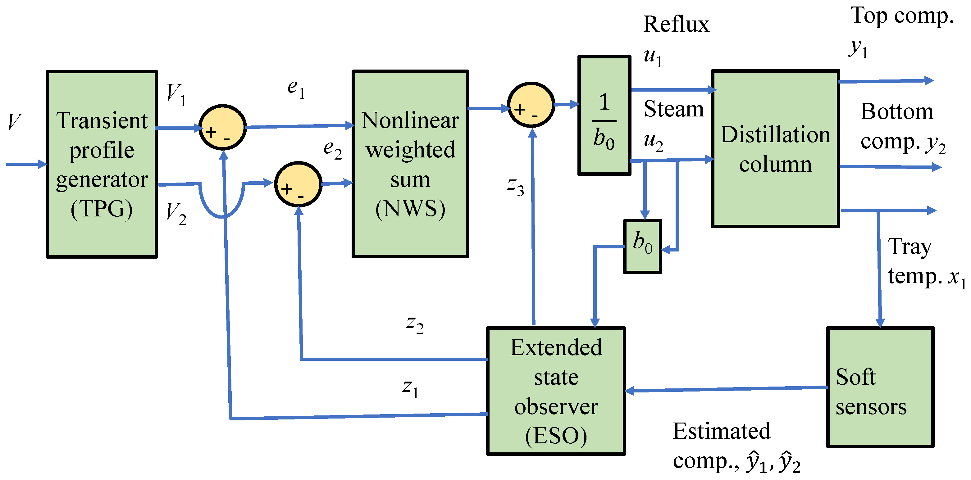
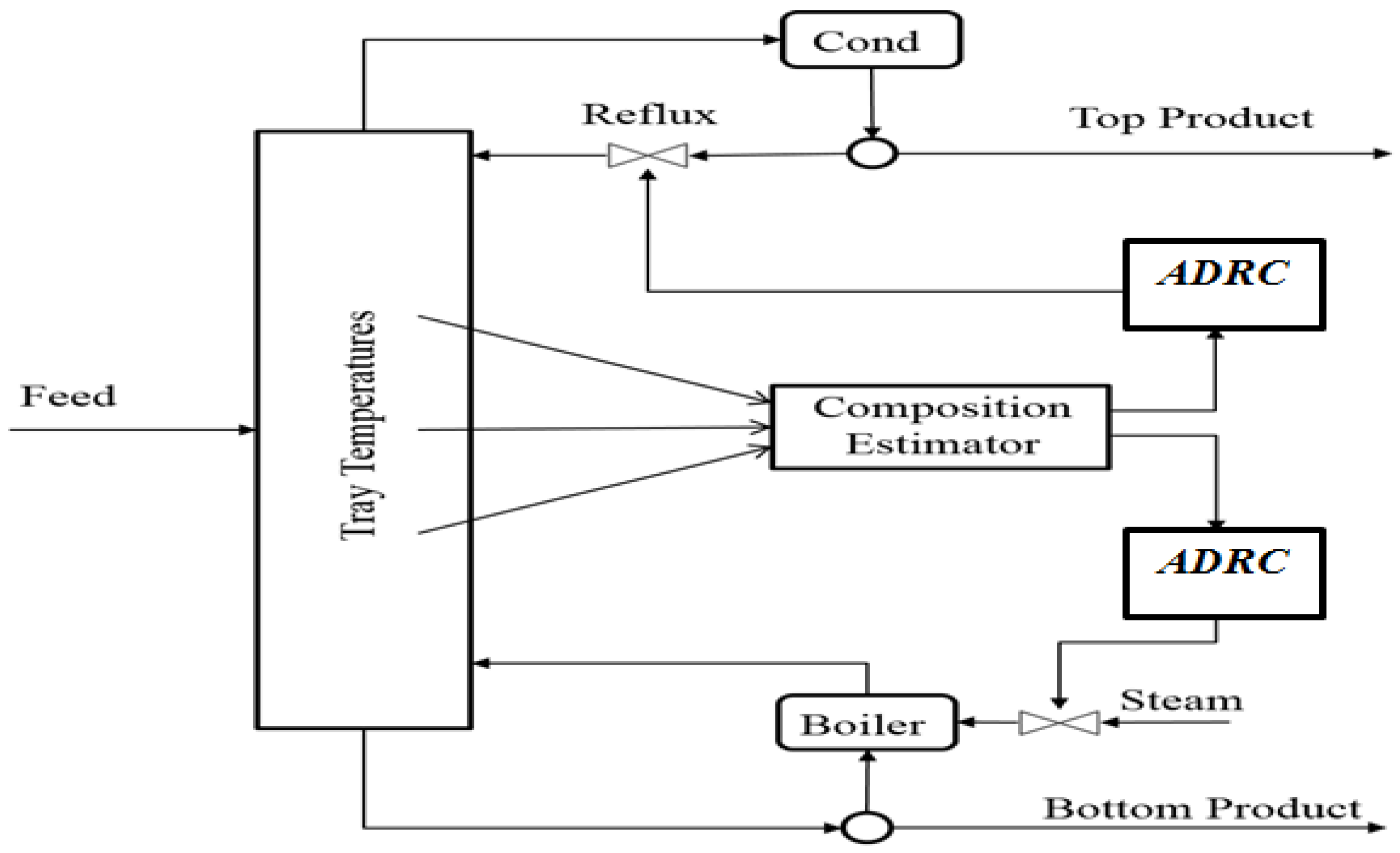
Figure 1 shows the ADRC structure which consists of three main parts: transient profile generator (TPG), non-linear weighted sum (NWS), and extended state observer (ESO).
TPG proposed in [
9] is a second order system that may produce smooth transition output process tracking the input set-point signal. Moreover, it is an effective technique to solve the conflict between avoiding overshoot and quickness in response of the controlled variable. Han [
9] proposed that TPG could be constructed by using the following equation.
In the above equation,
is the setpoint for the controlled variable,
is the desired trajectory,
is the derivative of the desired trajectory,
r is sometimes called tracking speed,
is the filtering factor, and
is the Han function [
9]. It can be noticed that the value of the parameter
r can be selected depending on the physical limitation of the plant. The speed of the transient profile can be slowed down or speeded up by selecting a suitable value of
r.
Usually, the conventional PID control employs a linear combination of proportional (present), integral (accumulative) and derivative (predictive) of the tracking errors. Moreover, other possibilities of combinations that might be much more effective are ignored. In addition, it usually needs the strategy on trade-off between fastness and overshoot of the control response. In order to avoid this contradiction, Han [
9] gives an alternative nonlinear function which depends on the magnitude of error signal to produce the control signal.
Systems are operating under different types of disturbances, among which the ones that have some impacts on the output signal are the most significant. As a result, the disturbances can be separated from the output signal by creating or defining new state which can be done by ESO. ESO generates the estimates of the unknown disturbances and unmeasured system states and then compensates them. Furthermore, ESO can enhance the system performance adaptability.
Consider the following 2nd order system [
9]:
where
y is the system output,
u is the manipulated variable for controlling
y, and
f(
x1,
x2,
de,
t) is a multivariable function of the states
x1 and
x2, the undesired external disturbance
de, and time
t. This function reflects the effect of the total disturbance
dt(
t). Using the total disturbance
dt(
t) as an additional state variable, Equation (2) can be organized as follows:
The states
x1(
t) to
x3(
t) can then be estimated by an ESO and the estimated states are denoted as
z1(
t) to
z3(
t) respectively. By inspecting
Figure 1 and in order to remove the impact of the total undesired disturbance on the controlled variable, the control law of the ADRC scheme can be written as:
where
g is the desired closed loop dynamics,
z3(
t) is the estimate of the total disturbance
dt(
t), and
b0 is an approximation of the parameter
b in Equation (2).
2.2. Overview of Inferential Control
The increasing availability of a wide range of sensors and data acquisition systems has led to a corresponding rise in the amount of data that can be logged through the computer control and monitoring systems of industrial processes. Hardware sensors give information on the process operation in terms of process variables, such as pressures, temperatures and flow rates, and product quality variables, such as composition and polymer molecular weight. Such sensors for product quality variables can be utilized to provide information on the quality of the final product in order to certify that it satisfies the customer requirements. However, many product quality variables cannot be easily and economically measured. Such sensors like composition analyzers usually possess large measurement delay and they are usually expensive. In many cases, the main product quality indicators are generally obtained by off-line sample analysis in a scientific laboratory. On-line quality analyzers such as gas chromatography and Near-InfraRed (NIR) are typically expensive and usually incur high maintenance cost [
13,
14]. Furthermore, significant delays and discontinuity associated with slowly processed quality measurements and laboratory analysis of on-line analyzers may reduce the efficiency and effectiveness of control policies. Instead of product composition control using composition analyzer and NIR, tray temperature control is broadly used to indirectly control product compositions. Moreover, tray temperature measurements are economic, reliable and virtually without any measurement time delays. However, utilizing single tray temperature to characterize the product composition has some drawbacks such as column pressure variation and feed rate or composition variation can significantly affect the correlation between tray temperatures and product compositions. In industrial processing plants, such restriction and limitations can have a severe impact on product quality.
In an effort to overcome the problems encountered in product composition measurement, soft sensing or inferential estimation techniques have acquired momentum recently as viable alternatives to hardware sensors in on-line process monitoring and control [
15]. In the last two decades, there has been rising interest and research in the development of soft sensors to provide regular on-line predictions of quality variables based on easy-to-measure process variables. Such soft sensors provide real time estimates of product quality variables and help to improve closed loop control performance and develop tight control policies [
16]. A soft sensor can be considered as a mathematical model that generates reliable real time estimates of unmeasured variables from easy-to-measure process variables [
16].
There are various advantages of soft sensors in the monitoring and control of industrial processes:
They provide more insight into the process through catching the information hidden in data;
They provide enhanced monitoring and control of industrial processes with the consequences of reducing environmental impact, enhancing productivity and energy efficiency, and improving business profitability through decreasing the production cost related to off-specification products;
They can be simply implemented on existing hardware. Moreover, on-line model identification algorithms can be utilized to adapt the model when plant characteristics change; and
They entail little or no capital costs such as installation cost, commissioning and management of the required infrastructure.
The design of soft sensors can be either by utilizing grey or black box identification approaches or on the basis of an analytical model. In the development of data-driven empirical model, least squares regression has been widely used. Nevertheless, when numerous input variables are used, this technique can become ineffective due to the strongly correlated nature of process variables. For instance, distillation column tray temperatures are closely correlated to each other and change together in the same pattern. Using linear regression techniques on such highly correlated process data leads to numerical errors due to close to singularity in the data covariance matrix. The common approach for tackling correlation problems is to select a few appropriate variables which are less correlated from each other [
17,
18,
19]. However, this simple technique is not optimal because the information in the discarded measurements might enhance the model performance.
Brosilow and co-workers [
17,
18] introduced a composition estimator called the Brosilow Estimator in which flow rates and temperatures were used for predicting unmeasured disturbance and then the estimated disturbances were utilized to predict product compositions. However, in recent years, product composition estimators have been designed using partial least squares regression (PLS) [
20,
21]. Mejdell and Skogested [
22] compared three linear model-based composition estimators of a binary distillation column. They briefed that good control performance might be reached with the steady state PCR (principal component regression) estimator. They found that the performance of the steady state PCR estimator is nearly good as the dynamic Kalman filter. Zhang [
23,
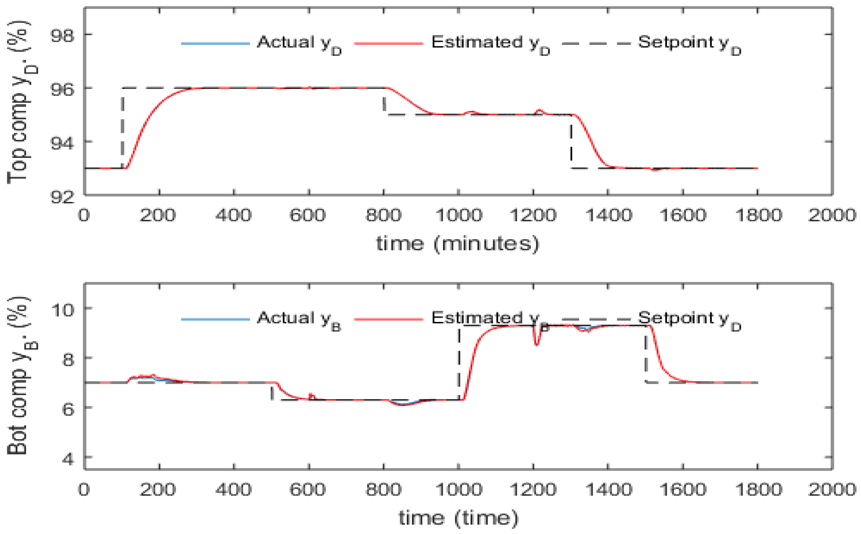
24] developed an inferential feedback control strategy for binary distillation composition control using PCR and PLS models. In these works, both top and bottom compositions are estimated via multiple tray temperature measurements and the estimated top and bottom product compositions are then used as feedback control signals.


