Abstract
Attention refers to the human psychological ability to focus on doing an activity. The attention assessment plays an important role in diagnosing attention deficit hyperactivity disorder (ADHD). In this paper, the attention assessment is performed via a classification approach. First, the single-channel electroencephalograms (EEGs) are acquired from various participants when they perform various activities. Then, fast Fourier transform (FFT) is applied to the acquired EEGs, and the high-frequency components are discarded for performing denoising. Next, empirical mode decomposition (EMD) is applied to remove the underlying trend of the signals. In order to extract more features, singular spectrum analysis (SSA) is employed to increase the total number of the components. Finally, some typical models such as the random forest-based classifier, the support vector machine (SVM)-based classifier, and the back-propagation (BP) neural network-based classifier are used for performing the classifications. Here, the percentages of the classification accuracies are employed as the attention scores. The computer numerical simulation results show that our proposed method yields a higher classification performance compared to the traditional methods without performing the EMD and SSA.
1. Introduction
Our brain receives a lot of sensory data generated from the environment every day. It is essential to pay attention when these data are being received in order not to miss them for further processing [1]. In fact, attention can be understood as an attribute or a feature of perceptual mechanisms and it is used to perform multiple cognitive control. Moreover, it is one of the five basic factors affecting intelligence [2], and it is used to evaluate the intellectual ability of a human.
Nowadays, both parents in major cities work outside during the daytime and leave their children at home after school. According to the survey, China has 23 million children being left at home, and the total number of children separated from their parents is increasing year by year. With the development of Internet technology, parents learn more about their children via electronic means. An attention assessment helps parents to find out the interests of their children, and plan the development of their children. Therefore, an attention assessment plays an important role in education development. On the other hand, according to the latest report conducted by the CDC in the United States, there is a child with the autism in every 44 children. In addition, the total number of autistic patients in China is more than 10 million, in which more than 3 million of the autistic patients are children. Moreover, the prevalence of ADHD in the world is as high as 6–14%. Nevertheless, severe cases of ADHD have a shorter life expectancy by 25 years. Furthermore, ADHD usually affects men more than women. More precisely, 12.9% of men and 4.9% of women are diagnosed with ADHD. In fact, the attention assessment also plays an important role in the diagnosis of ADHD and autism. This is because participants with autism highly concentrate on their work if they are interested in. On the other hand, they are highly immersed in their work if they are not interested in.
It is worth noting that different medical officers sometimes give very different attention scores to the same participant doing the same task at the same time. Hence, it is very difficult to have a subjective and reliable attention assessment. As EEGs reflect the electrophysiological activity of the neurons [3], they contain the physiological and pathological information of the human brain. In particular, the α waves are related to the attention levels when the participants work on a particular task, the β waves are related to the emotional and cognitive status of the participants [4], the θ waves are related to the moral status of the participants [5], and the δ waves are related to the attention levels when the participants perform mental tasks [6]. Hence, EEGs are widely used for the understanding of brain activities [7] and the analysis of human emotions due to personality inference. As a result, EEGs are widely used for performing sleep-stage classification, monitoring physiological state, applying intelligent rehabilitation therapy, identifying personality characteristics [8], as well as performing the diagnosis and treatment of sleep-related diseases [9] via brain-computer interface (BCI) systems [10,11]. Recently, EEGs are employed for performing automatic attention assessment [12]. In particular, the participants wear a wearable and portable device for acquiring the EEGs when they are playing an electronic game. Then, an analysis is performed based on the EEGs. An indication of the attention level is reflected in the electronic game. However, this attention assessment is designed only for participants who play electronic games [13]. Nevertheless, children are not only playing electronic games, but they also do other activities at home. Therefore, it would be useful if the attention assessment can be performed for participants doing other activities. To address this issue, this paper proposes an attention assessment method for participants doing other activities.
At present, single-channel EEGs are used for the consumer-level applications. This is because single-channel EEGs are portable and easily acquired. In addition, the costs of single-channel EEG devices are affordable to consumers. More importantly, single-channel EEGs can operate at higher sampling rates under the same data transmission rate. This will yield a better classification performance. Hence, this paper employs single-channel EEGs for performing the classification.
It is worth noting that the traditional method uses infinite impulse response filters such as the Butterworth filter to suppress noise. However, these filters introduce nonlinear phase distortion to the extracted waves. Therefore, the classification performance based on the extracted waves is degraded. To address this issue, this paper performs the FFT on the EEGs. Then, only the corresponding FFT coefficients are retained. This operation behaves similarly to idea filtering. As the retained FFT coefficients are conjugate pairs, no phase distortion is introduced. Finally, the inverse FFT is computed to obtain the denoised EEGs.
EMD is a nonlinear and adaptive signal representation method that decomposes a signal into the sum of a small number of interpretable components. It has been used for performing the underlying trend extraction. In particular, as the last several components of the EMD exhibit slowly varying oscillations, discarding these components can remove the underlying trend of the EEGs due to the motion artifacts. Hence, this paper employs the EMD for removing the underlying trend of the EEGs.
To perform the four sleep-stage classifications [14,15], the traditional methods are based on decomposing the EEGs into the β waves, α waves, θ waves, γ waves, and δ waves. Then, the features are extracted from these brain waves. However, the total number of the extracted features is very limited. As a result, the classification accuracy is low. To address this issue, it is worth noting that the SSA is also a nonlinear and adaptive signal representation method that decomposes a signal into the sum of a small number of interpretable components. Hence, this paper employs the SSA to decompose each EMD component into further components. As the total number of components is increased, more features can be extracted. In particular, this paper also extracts 11 different features from each group of SSA components. The computer numerical simulation results show that our proposed method greatly improves the classification performance. In fact, SSA has been used for processing single-channel EEGs [16] and EOGs [17], as well as for performing high-precision seizure detection and EEG classification [18].
It is worth noting that the automatic attention assessment is in fact a regression problem. The common regression methods include the logistic regression method, polynomial regression method, and ridge regression method. Nevertheless, these regression methods require subjective and reliable reference values for the attention levels. Hence, the results obtained via these regression methods are not reliable. To address this issue, this paper proposes a classification approach to perform the attention assessment. In this case, the reference attention levels are not required.
The objective of this paper is to propose a method for performing a subjective and effective attention assessment with participants conducting various activities. The novelty and contribution of this paper are to propose a classification method to perform the regression task. In this case, reference values from medical officers are not required. In addition, this paper proposes to employ SSA to increase the total number of features to improve the classification accuracy. The outline of this paper is as follows: Section 2 reviews the existing nonlinear time–frequency analysis techniques. Section 3 presents our proposed method. Section 4 shows the computer numerical simulation results. Finally, a conclusion is summarized in Section 5.
2. Review on the Existing Nonlinear Time–Frequency Analysis Techniques
2.1. SSA
SSA is a recently proposed method for performing nonlinear and adaptive signal decomposition. Since no pre-defined kernel is required [9], it is found to be very useful for analyzing signals. As a result, it is widely used in the mathematics, physics, finance, meteorology, social science, and biomedical signal processing communities.
The procedures for performing the SSA are summarized as follows: First, it constructs a trajectory matrix using the given signal. Second, singular value decomposition (SVD) is applied to the trajectory matrix, and various components, such as the underlying trend, periodic, and noise components, are obtained. Then, the useful components are retained, while the rest of the components are discarded. Finally, diagonal averaging is performed. In particular, let be the length of a signal. Let be the vector of this signal. Let be the window length. Here, . Define . Let for be the th segment of the signal. Let [,,…,] be the trajectory matrix such that the th column of is . That is,
It is worth noting that is a Hankel matrix. The second step for performing the SSA is to apply SVD to to obtain the various components. Let and be the left unitary matrix and the right unitary matrix obtained by applying SVD to , respectively. However, the computational complexity is very large if SVD is applied to directly. To address this issue, SVD is applied to the covariance matrix to obtain . Then, is derived based on both and . Let be the diagonal matrix obtained by performing SVD on . It is worth noting that the singular values and the singular vectors of are the squares of the singular values and the left singular vectors of X, respectively. That is,
Let be the diagonal elements in . That is, . Here, are sorted in descending order. That is, . Let and . Let
It can be shown that can be represented as the sum of . That is,
It can be shown that
Next, are grouped based on a certain criterion. Assume that the index set {} is partitioned into a finite number of disjoint subsets. Let M be the total number of these disjoint subsets. Let be these disjointed subsets. Let . It can be shown that can be represented as
However, only some terms are summed together to construct a useful signal. The third step for performing the SSA is to perform diagonal averaging on This process involves representing as a one-dimensional vector. It can be seen from (6) that the sum of the elements in the same positions of all is equal to the corresponding element in the trajectory matrix. Hence, applying diagonal averaging on each to obtain the corresponding one-dimensional SSA component and then summing up all these one-dimensional SSA components together is equivalent to applying diagonal averaging to the trajectory matrix. Therefore, diagonal averaging is an inverse operation with respect to the Hankelization. Let be an element in the ath row and the bth column of . Let be the th element in the th one-dimensional SSA component. Performing diagonal averaging involves computing the average of all the elements along the th off-diagonal of as shown in Figure 1. Here, .
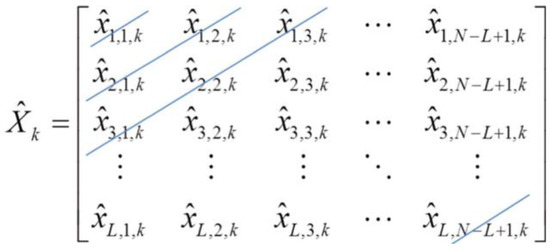
Figure 1.
The diagonal averaging operation.
From Figure 1, we have:
Mathematically, diagonal averaging is equivalent to performing the following operations [19,20]:
Let be the obtained one-dimensional SSA component.
2.2. EMD
Suppose that a signal is composed of a finite number of components. EMD is an algorithm for finding these components. More precisely, EMD is used to represent a signal as the sum of various components. These components are called intrinsic mode functions (IMFs). If the IMFs are different from the actual components, then mode mixing occurs. Here, the EMD does not require any pre-defined kernel for performing the decomposition. As the IMFs are only dependent on the signal itself, EMD is an adaptive signal decomposition method. On the other hand, it is worth noting that the decomposition is based on the time-scale characteristics of the given signal. As a signal with more extrema contains more high-frequency components than a signal with less extrema, EMD exploits the time–frequency characteristics of the signal. These excellent properties of EMD facilitate many science and engineering applications [21,22,23].
A function is said to be an IMF if it satisfies the following two conditions:
- (1)
- The absolute difference between the total number of extrema and the total number of zero-crossing points is no more than 1.
- (2)
- The area under the curve between two consecutive extrema is zero.
The procedures for performing the EMD are as follows:
- Step 1
- Initialization: Let and .
- Step 2
- Compute the IMFs: Let (t) be the nth IMF. It is found using the following procedures:
- (a)
- Let and .
- (b)
- Find the maxima and minima of .
- (c)
- The cubic spline function is used to interpolate among the maxima and minima to obtain the upper and lower envelope of , respectively. Let and be the upper and lower envelope of , respectively.
- (d)
- Calculate the mean of and . Let be this mean. That is, .
- (e)
- Performing the sifting process via subtracting from . That is, .
- (f)
- A criterion is imposed to terminate the algorithm. Let . If , then let and go to Step 3. Otherwise, increment the value of and go back to Step 2b.
- Step 3
- Let .
- Step 4
- If is an IMF or a monotonic function, then the decomposition is completed. Otherwise, increment the value of and go back to Step 2a.
Let be the total number of the obtained IMFs and be the residue. Then, can be represented as the sum of these IMFs and the monotonic residue as follow:
For simplicity reasons, let .
3. Our Proposed Method
Figure 2 shows the block diagram of our proposed method. The main idea of our proposed method is as follows: First, in order to perform the attention assessment, two sets of EEGs are acquired. They are the sets of EEGs where the participants perform different activities under the concentration state and the immersion state. Second, since the useful information of the EEGs is localized between 0 Hz and 50 Hz and the components outside 50 Hz can be understood as noise, FFT is used to perform the denoising. In particular, the FFT coefficients between 0 Hz and 50 Hz are retained and those outside 50 Hz are discarded. Third, EMD is used to perform the detrending. Fourth, FFT is applied again to obtain the various types of the brain waves. In particular, nine brain waves are obtained. Fifth, SSA is applied to decompose each brain wave and the detrended EEG into the various SSA components. Then, the grouping is performed. Overall, there are 22 grouped SSA components for each detrended EEG. Sixth, the features are extracted from each SSA grouped component. Seventh, the BP neural network-based classifier, random forest based-classifier, and SVM-based classifier are used to perform the training. Finally, the class of each test EEG is estimated. Due to randomness, the above operations are performed three times. The accuracy based on the average of these three classification results is taken as the final result.
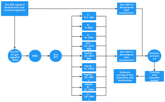
Figure 2.
The block diagram of our proposed method.
3.1. Data Acquisition
It is worth noting that no database for performing the activity recognition using single-channel EEGs operated at 512 Hz can be found on the Internet. Hence, it is difficult to perform a fair comparison using the data in the public domain. Therefore, this paper builds a new database and the data is available on the Internet at this link: https://www.aliyundrive.com/s/Qhuc1ZFRkLr, accessed on 18 December 2022. In particular, the EEGs are acquired from 12 participants, including 9 boys and 3 girls. There were 9 participants from Guangzhou and 3 participants from Hong Kong. All of them have conducted the body test and they are certificated with a good health status. Each participant conducts seven activities. These seven activities are drawing, eating, doing computer exercises, playing electronic games, reading, playing toys, and watching television. Each activity is conducted twice with each time lasting for around 10 to 15 min. Here, each activity conducted at the first time and the second time are under the concentration state and the immersion state, respectively. For conducting the activities under the concentration state, there is no interruption to the participants. In addition, the surrounding environment is particularly quiet without any noise so that the participants can easily focus on the activities they performed. Moreover, since it is difficult for the participants to focus on the activities for a long period of time, different activities conducted by the individual participants are carried out on different days. Here, it is assumed that the attentions of the participants are independent of the day when they perform the activities. For conducting the activities under the immersion state, the participants are disturbed when they conduct these activities. For example, the ears of the participants are disrupted by feathers or they are talking to one another all the time.
Moreover, the NeuroSky TGAM1 chip is used as the sensor to acquire the single-channel EEGs with the sampling frequency operating at 512 Hz. Figure 3 shows the acquisition device. This EEG device has three contact points. The sensor is placed at the TP10 location near the right ear lobe because there is no bone there. Hence, the EEGs can be sensed by the electrode more easily. On the other hand, the other two contact points are the reference point (REF) and the ground point (GND). They are located at the forehead because the contact surface is large there. Hence, it can avoid poor contact. WiFi is used to transmit the EEGs acquired from this device to the xampp server built in the computer. The EEGs are segmented into pieces using an ideal rectangular window. Each piece of the EEGs lasted for one second. Hence, each piece of the EEGs consists of 512 points. Here, each piece of the EEGs is regarded as an individual sample. Within one second, it is assumed that the attention level of the participants remains unchanged. In this paper, the pieces of the EEGs acquired under the poor contact condition are removed. Table 1 and Table 2 show the total numbers of the retained samples when different participants are conducting different activities under the concentration state and the immersion state, respectively. It is found that about 13 to 806 pieces of the EEGs are retained.
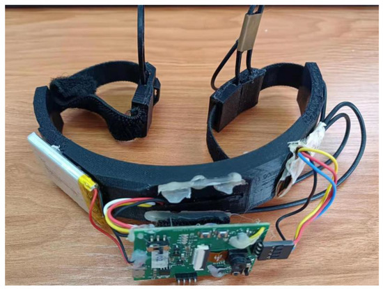
Figure 3.
The acquisition device.

Table 1.
The total numbers of the retained samples when different participants are conducting different activities under the concentration state.
Table 2.
The total numbers of the retained samples when different participants are conducting different activities under the immersion state.
3.2. FFT-Based Denoising
Figure 4 shows an example of a sample of the EEG when Danny is conducting the drawing activity under the concentration state. It is well known in the EEG community that the useful information of the EEG is localized in the frequency band between 0.5 Hz and 49 Hz. However, it can be seen from Figure 4 that there is a high-frequency noise above 50 Hz contaminating the EEG. Hence, it is required to remove this high-frequency noise. Although different IMFs are localized in different frequency bands, the IMFs have leakages in the frequency domain because these IMFs are not bandlimited. Moreover, as the mode-mixing phenomenon occurs [21,23], the obtained IMFs are not the corresponding brain waves. To address this issue, the FFT approach is applied. That is, the FFT is applied to the EEG and those coefficients higher than 50 Hz are set to zero. As the remained coefficients are bandlimited, this is equivalent to applying the ideal lowpass filtering to the EEG. In this case, the high-frequency artifacts are eliminated. Moreover, the corresponding brain waves can be extracted directly via the FFT approach.
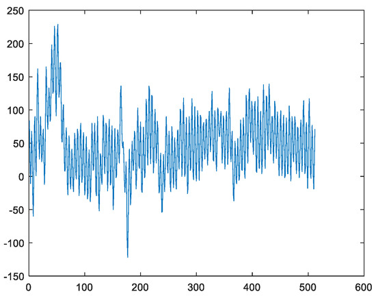
Figure 4.
An example of a sample of the EEG when Danny is conducting the drawing activity under the concentration state.
3.3. Removing the Underlying Trend via the EMD
It is worth noting that the eye and muscular activities would introduce drift to the acquired EEGs. In fact, this drift can be characterized by the underlying trend of the EEGs. On the other hand, the EMD represents a signal as the sum of its IMFs with different IMFs localized in different frequency bands. It is well known that the underlying trend of a signal can be characterized by the sum of its last several IMFs. This is because the last several IMFs usually have large time scales and they are also low-frequency components. These properties are the same as those of the underlying trend [24]. To address this issue, this paper applies EMD to the denoised EEGs obtained in Section 3.2, and the last several IMFs corresponding to the underlying trend components and the low-frequency components of the EEGs are discarded. As a result, the effects of the eye and muscular activities are eliminated. More precisely, this paper removes the last two IMFs. Figure 5 shows the denoised EEG and the corresponding detrended EEG. It can be seen from Figure 5 that the average value of the denoised signal is not equal to zero. This implies that there is an underlying trend in the denoised signal. On the other hand, this is not the case for the detrended signal. This implies that the underlying trend of the denoised signal is effectively removed via the EMD approach.
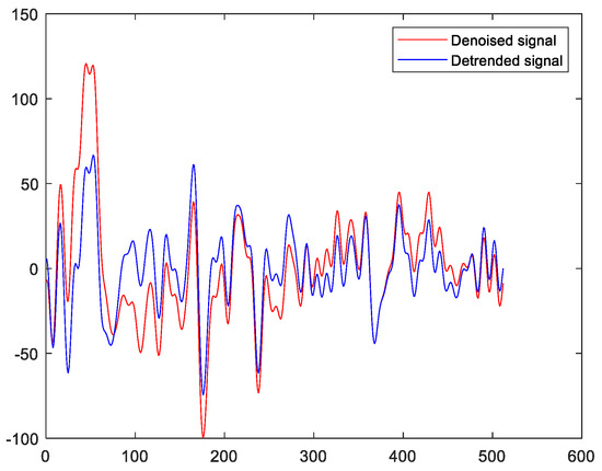
Figure 5.
The denoised signal and the detrended signal.
3.4. Feature Extraction Based on the SSA
The EEGs consist of the various brain waves localized in different frequency bands. The frequency band of the δ wave is between 0.5 Hz and 4 Hz, that of the θ wave is between 4 Hz and 8 Hz, that of the α wave is between 8 Hz and 12 Hz, that of the sensory motor rhythm (SMR) wave is between 12 Hz and 14.99 Hz, that of the mid β wave is between 15 Hz and 19.99 Hz, that of the high β wave is between 20 Hz and 30 Hz, that of the low β wave is between 12 Hz and 19 Hz, that of the whole β wave is between 12 Hz and 30 Hz, and that of the γ wave is between 30 Hz and 49 Hz. To extract these waves from the EEG, an FFT approach is applied to the detrended EEGs obtained in Section 3.3. That is, the FFT is applied to the EEGs and the coefficients outside the corresponding frequency bands are set to zero. Then, the inverse FFT (IFFT) is applied to the processed signals to obtain the corresponding waves. Figure 6 shows the obtained brain waves when Danny is conducting the drawing activity under the concentration state.
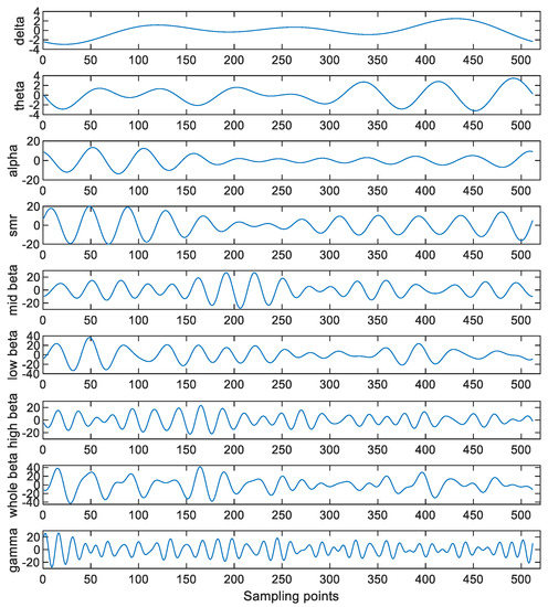
Figure 6.
The obtained brain waves when Danny is conducting the drawing activity under the concentration state.
It is worth noting that the FFT has been applied twice as discussed in Section 3.2 and Section 3.4, the first time to perform the denoising, the second time to extract the various waves from the denoised and the detrended EEGs. In fact, these two FFT operations cannot be combined. This is because the duration of the samples is one second. Hence, the frequency resolution of the FFT coefficients is 1 Hz. Even when the DC frequency of the samples is set to zero, the detrended performance is not good. Therefore, EMD is required to be employed to remove the underlying trend of the EEGs, where the detrended operation is performed between these two FFT operations.
Table 3 shows some common human behaviors and the brain waves responsible for these human behaviors. As the brain waves are related to the human behaviors, this paper extracts the features from these brain waves for performing the attention assessment. On the other hand, it is worth noting that more than one component can be obtained via performing the SSA. Hence, more features can be extracted by applying the SSA to these brain waves. In particular, the SSA is applied to both the detrended EEGs and the decomposed brain waves. Here, L is set at 6 for the detrended EEGs, so there are six SSA components for each detrended EEG. Then, these six SSA components are categorized into four groups. More precisely, the first component is put into the first group. The second and third components are put into the second group. The fourth and fifth components are put into the third group. Finally, the sixth component is put into the fourth group. Figure 7 shows these four groups of the SSA components. Moreover, L is set at 2 for these decomposed brain waves. Figure 8 shows these two sets of the SSA components decomposed from the brain waves. Since there are four groups of the SSA components decomposed from each detrended EEG as well as two sets of the SSA components decomposed from each brain wave and there are nine brain waves for each detrended EEG, there are 22 components in total for each detrended EEG.
Table 3.
The common human behaviors and the brain waves responsible for these human behaviors.
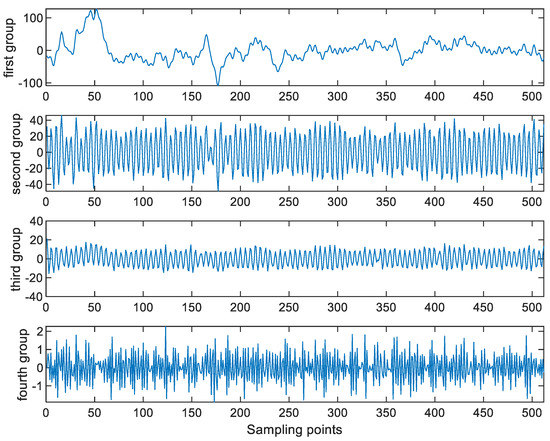
Figure 7.
The four groups of the SSA components.
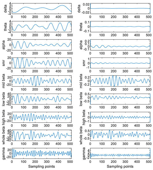
Figure 8.
These two sets of the SSA components decomposed from the brain waves of a detrended EEG.
Since the amplitudes of different brain waves are different, the amplitudes and energies of the SSA components are not used as features for performing the attention assessment. Instead, this paper employs other physical quantities such as the approximate entropy, the mean, the variance, the interquartile range, the mean absolute deviation, the range, the skewness, the kurtosis, the norm, the norm, and the norm of the SSA components of each detrended EEG as the features. The details of these physical quantities are presented below.
3.4.1. Approximate Entropy
The approximate entropy is a physical quantity that is robust to the noise and the interference. Hence, it has been used to estimate the characteristics of the distribution of both a short random signal and a short deterministic signal acquired at both the noise environment and the interference environment [25]. On the other hand, as the EEGs behave like a random signal, the approximate entropy should be effective for analyzing the EEGs. However, it has not been used for performing the attention assessment yet. Therefore, this paper explores the feasibility and effectiveness of using the approximate entropy for performing the attention assessment. Let be an SSA component. Let be the length of the marginal window of the SSA. Then, the SSA component is divided into a finite number of sub-sequences. Let be the th sub-sequence. That is, . Let be the length of this SSA component. Let be the total number of sub-sequences. Obviously, . Let be the distance between X(i) and X(j). Here, is defined as the maximum absolute difference between X(i) and X(j). Let be a value between 0.25 and 0.75. In this paper, is chosen as 0.5. Let be the standard deviation of the SSA component. Let be a threshold. Then, is selected as . For each , there are distances. Let be the percentage of the total number of distances having values greater than P. Let be the logarithmic average of . Finally, increment the value of m and repeat the above procedures. Then, we have . Define as the approximate entropy.
3.4.2. Mean and Variance
Let be the mean of x(t).
Let be the variance of x(t).
3.4.3. Interquartile Range
Let be the ordered EEG sorted in ascending order. Let Q1, Q2, and Q3 be the lower quartile, the median, and the upper quartile of , respectively. That is, they are the 25th percentile, the 50th percentile, and the 75th percentile of , respectively. Let IQR = Q3 − Q1.
3.4.4. Mean Absolute Deviation
Let be the mean absolute deviation of .
3.4.5. Range
Let be the range of .
3.4.6. Skewness and Kurtosis
Let be the skewness of .
Let be the kurtosis of .
3.4.7. L1 Norm, Norm, and Norm
Let be the norm of .
Let be the norm of .
Let be the norm of .
It is worth noting that there are 11 features for each SSA component. As there are 22 components for each detrended EEG, the length of the feature vector is 242.
In order to verify whether these features are effective for performing the attention assessment, the ANOVA is performed on these features. The implementation was conducted using the Matlab statistical toolbox with the confidence level set at 95%. Let P be the probability of producing a statistical significance. Then, the power of the hypothesis testing refers to the percentage of the cases where P is smaller than one minus the confidence level. In this case, if P is less than 0.05, then these features are statistically significant. The hypothesis test results are shown in Table 4. It can be seen from Table 4 that many values of P are less than 0.05. In particular, it can be seen from the Table 4 that 195 values of P were less than 0.05. Hence, the power of the hypothesis testing was 80.58%. It can be concluded that these features are effective.
Table 4.
The values of P corresponding to different features extracted from the SSA components of a detrended EEG.
3.5. Classification
It is challenging to assess human attention via EEGs. This is because there is no standard method to score the degree of attention of the participants when they conduct the various activities. To address this issue, this paper employs the features extracted from the EEGs acquired from the various participants conducting the various activities under both the concentration state and the immersion state to train the classifiers. Here, three common classifiers, namely the random forest-based classifier, the SVM-based classifier, and the BP neural network-based classifier are employed for performing the classification. However, the total number of EEGs for a particular activity corresponding to the concentration state is different from that corresponding to the immersion state. Hence, there is a data imbalance issue. To address this issue, this paper employs 30% of all the EEGs for each activity for performing the testing. For the remaining 70% of all the EEGs for each activity, it first forms a preliminary training set. Then, only a part of the EEGs in this preliminary training set is taken out to construct the model for performing the classification. In particular, the total number of EEGs for each activity corresponding to the concentration state used for performing the training is taken to be the same as that corresponding to the immersion state. After performing the classification, the percentage of the total number of the EEGs that are classified correctly is computed. Here, it is assumed that the classification error is only due to the change of the state when the participant conducts the corresponding activity. Therefore, this percentage can be used to score human attention.
3.5.1. Random Forest-Based Classifier
The random forest is a bagging and a decision tree-based machine learning method [26]. Assume that there are N samples in the training set. The bootstrap method is used to select a sample at each iteration from these N samples randomly. To determine the splitting nodes in the decision tree, some features are selected randomly. The Gini index is computed to determine the optimal splitting node. These procedures are repeated until it cannot be further split. Finally, the above procedures are repeated and these decision trees form a random forest. Figure 9 shows the process for the formation of the random forest.
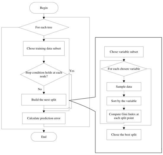
Figure 9.
The procedures for the formation of the random forest.
A decision tree in the random forest is a weak learner. It makes an individual decision. The overall decision is made by voting the majority decision among all the individual decisions. Since the samples are selected randomly and the features in each sample are also selected randomly, this approach can raise the generalization ability of the model.
3.5.2. BP Neural Network-Based Classifier
A multi-layer feedforward neural network consists of one input layer, one or more than one implicit layer, and one output layer. The implicit layer is also called the hidden layer. Training the neural network is finding the parameters in the neural network. The BP neural network is a neural network with its parameter trained by the error reverse propagation algorithm. In particular, the training composes of two major steps. The first step is the forward propagation of the signal and the second step is the BP of the error. For the first step, the input at the input layer is processed layer by layer and yields the output at the output layer. For the second step, if the output at the output layer does not match the desired output, then the error is back-propagated to the input. That is, the output is transmitted from the output layer back to the input layer through the hidden layer based on the error between the desirable output and the actual output. Here, the error is shared to all the nodes in all the layers. The weights and the thresholds of the nodes are updated via the fastest descent-based learning rule so that the total error in all the nodes is minimized. Figure 10 shows the diagram of the BP neural network [27].
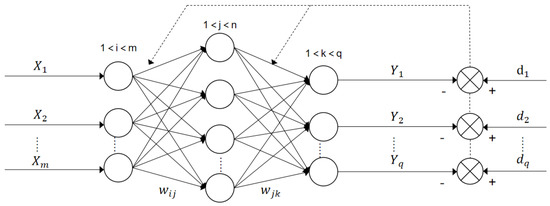
Figure 10.
The BP neural network.
3.5.3. SVM-Based Classifier
As the SVM is a powerful classification method, it has been widely used in many real-world pattern recognition and the machine learning applications [28]. The SVM maps the input feature vectors in a high dimensional space to the feature vectors in a low dimensional space via a nonlinear kernel function. As the dimension of the output of the kernel function is reduced, the required computational power for computing the product of the outputs of two kernel functions () is lower than that for the inner product between the weight matrix and the feaure vector. Hence, the SVM can significantly reduce the required computational power. After performing the nonlinear mapping, the linear classification method is applied in the low dimensional space. In general, the linearly separable recognition problem can be classified correctly using a linear hyperplane. To find this optimal linear hyperplane, the optimization approach is employed. That is, the maximum distance between the feature vectors and the linear hyperplane is minimized. However, the feasible set of the optimization problem is empty if the recognition problem is nonlinearly separable. To address this issue, the penalty factor is introduced to modify the the loss function and the classification interval. Nevertheless, the classification performance of the SVM is highly dependent on the choice of the kernel function and the error penalty factor.
4. Computer Numerical Simulation Results
Table 5 and Table 6 show the percentages of the classification accuracies for 12 participants performing the various activities under the concentration state and the immersion state via the traditional methods, respectively. Here, the traditional methods refer to the methods of performing both the FFT-based denoising and the classifications via the above three classifiers but without applying the SSA and the EMD to the denoised EEGs. On the other hand, Table 7 and Table 8 show the percentages of the classification accuracies for these 12 participants performing the various activities under the concentration state and the immersion state via our proposed method, respectively. Here, our proposed method refers to the method of performing the FFT-based denoising, applying both the SSA and the EMD to the denoised EEGs, as well as performing the classifications via these three classifiers. Moreover, the average percentages of the classification accuracies over both these 12 participants and over these three classifiers for each activity under the concentration state and the immersion state yielded by the traditional methods and our proposed method are shown in Table 5, Table 6, Table 7 and Table 8. It can be seen from these tables that the average percentages of the classification accuracies over both these 12 participants and over these three classifiers yielded by our proposed method are higher than those yielded by the traditional methods for all the activities as well as for both the concentration state and the immersion state. Furthermore, it is found that the highest score recorded in the concentration state yielded by our method is 100. This demonstrates that our proposed method yields a better classification performance.
Table 5.
The percentages of the classification accuracies for 12 participants performing the various activities under the concentration state yielded by the traditional methods.
Table 6.
The percentages of the classification accuracies for 12 participants performing the various activities under the immersion state via yielded by the traditional methods.
Table 7.
The percentages of the classification accuracies for 12 participants performing the various activities under the concentration state yielded by our method.
Table 8.
The percentages of the classification accuracies for 12 participants performing the various activities under the immersion state via yielded by our method.
Moreover, for the activities conducted in the concentration states by our proposed method, the eating activity has the lowest average score which is 68.63, the playing toy activity has the second lowest average score which is 74.24, the drawing activity has the third lowest average score which is 83.66, the playing electronic game activity has the intermediate average score which is 86.26, the watching television activity has the third highest average score which is 86.61, the doing computer exercise activity has the second highest average score which is 88.60, and the reading activity has the highest average score which is 88.75. For the activities conducted in the concentration states by the traditional method, the eating activity has the lowest average score which is 68.07, the playing toy activity has the second lowest average score which is 69.53, the drawing activity has the third lowest average score which is 74.30, the playing electronic game activity has the intermediate average score which is 80.35, the watching television activity has the third highest average score which is 80.67, the doing computer exercise activity has the second highest average score which is 82.26, and the reading activity has the highest average score which is 82.37. For the activities conducted in the immersion states by our proposed method, the eating activity has the lowest average score which is 72.33, the playing toy activity has the second lowest average score which is 76.97, the watching television activity has the third lowest average score which is 86.80, the drawing activity has the intermediate average score which is 86.96, the playing electronic game activity has the third highest average score which is 88.04, the doing computer exercise activity has the second highest average score which is 88.05, and the reading activity has the highest average score which is 91.34. Here, it can be seen that there are the similar sorting orders for the activities yielded by both our proposed method and the traditional methods for both the concentration state and the immersion state. This demonstrates that our proposed method is reliable. Moreover, as it is required to pay more attention when performing the reading activity and the doing computer exercise activity compared to performing the eating activity and the playing toy activity, the obtained results are reasonable.
Furthermore, it is worth noting that it is not necessarily true for the average percentages of the classification accuracies over both these 12 participants and over these three classifiers for performing the various activities yielded by both our proposed method and the traditional methods under the concentration state to be higher than those under the immersion state.
Figure 11 shows the average percentages of the classification accuracies over both these 12 participants performing the various activities yielded by both our proposed method and the traditional methods with different classifiers under the concentration state. Likewise, Figure 12 shows the average percentages of the classification accuracies over both these 12 participants performing the various activities yielded by both our proposed method and the traditional methods with different classifiers under the immersion state. For the concentration state, the average percentages of the classification accuracies over both these 12 participants performing the various activities yielded by our proposed method based on the the BP neural network-based classifier, the random forest-based classifier, and the SVM-based classifier models are 82.04, 84.99, and 80.11, respectively. The average percentages of the classification accuracies over both these 12 participants performing the various activities yielded by the traditional method based on the the BP neural network-based classifier, the random forest-based classifier, and the SVM-based classifier models are 74.85, 79.80, and 78.46, respectively. For the immersion state, the average percentages of the classification accuracies over both these 12 participants performing the various activities yielded by our proposed method based on the the BP neural network-based classifier, the random forest-based classifier, and the SVM-based classifier models are 81.82, 87.86, and 85.65, respectively. The average percentages of the classification accuracies over both these 12 participants performing the various activities yielded by the traditional method based on the BP neural network-based classifier, the random forest-based classifier, and the SVM-based classifier models are 74.67, 79.87, and 79.53, respectively. It can be seen from these two figures that the random forest-based classifier yields the highest average percentages of the classification accuracies compared to the SVM-based classifier and the BP neural network-based classifier for both the concentration state and the immersion state as well as for both our proposed method and the traditional method. This is because the random forest introduces randomness in the selection of both the feature vectors and the features in the generation of the forest. Thus, the effect of the overfitting is small.
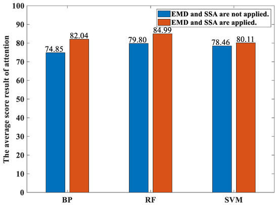
Figure 11.
The average percentages of the classification accuracies over both these 12 participants performing the various activities yielded by both our proposed method and the traditional methods with different classifiers under the concentration state.
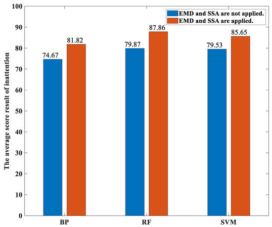
Figure 12.
The average percentages of the classification accuracies over both these 12 participants performing the various activities yielded by both our proposed method and the traditional methods with different classifiers under the immersion state.
It is worth noting that the duration of each sample shown in the above computer numerical simulations is one second. It is interesting to see if the percentages of the classification accuracies would depend on the duration of the samples. Now, the duration of each sample is changed to three seconds, five seconds, and ten seconds. The percentages of the classification accuracies yielded by our proposed method via the various classifiers based on the EEGs at different durations of the samples acquired from Hejian performing the reading activity under the concentration state are shown in Table 9. It can be seen from Table 9 that the percentages of the classification accuracies are almost the same. In addition, the percentages of the classification accuracies based on the duration of the samples lasting for one second are the highest compared to the other durations of the samples for both the random forest-based classifier and the SVM-based classifier. Moreover, as some of the existing works are also based on the EEGs with the duration of the samples being equal to one second [29,30], this paper chooses the duration of the samples as one second.
Table 9.
The percentages of the classification accuracies yielded by our proposed method via the various classifiers based on the EEGs at different durations of the samples acquired from Hejian performing the reading activity under the concentration state.
Moreover, the total time taken required for performing the attention assessments for each individual for performing each activity under both the concentration state and the immersion state via the traditional methods with all three classifiers is shown in Table 10. Likewise, the total time taken required for performing the attention assessments for each individual for performing each activity under both the concentration state and the immersion state via our proposed method with all three classifiers is shown Table 11. Although our proposed method takes a longer time for performing the attention assessments compared to the traditional methods due to the time required for performing the extra operations on the SSA and the EMD, the extra time is affordable for medical applications.
Table 10.
The total times required for performing the attention assessments for each individual for performing each activity under both the concentration state and the immersion state via the traditional methods with all three classifiers.
Table 11.
The total times required for performing the attention assessments for each individual for performing each activity under both the concentration state and the immersion state via our proposed method with all three classifiers.
Figure 13 and Figure 14 show the relationships between the percentage of the classification accuracy and the total number of neurons in the hidden layer of the BP neural network in our proposed method trained using the EEGs acquired from Hejian performing the reading activity under the concentration state on the first day and on the second day, respectively. It can be seen that the highest percentage of the classification accuracy is yielded when 10 neurons are used in the hidden layer of the BP neural network regardless of whether the EEGs are acquired on the first day or on the second day. Hence, this paper employs 10 neurons in the hidden layer of the BP neural network.
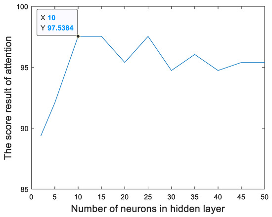
Figure 13.
The relationship between the percentage of the classification accuracy and the total number of neurons in the hidden layer of the BP neural network in our proposed method trained using the EEGs acquired from Hejian performing the reading activity under the concentration state on the first day.
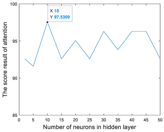
Figure 14.
The relationship between the percentage of the classification accuracy and the total number of neurons in the hidden layer of the BP neural network in our proposed method trained using the EEGs acquired from Hejian performing the reading activity under the concentration state on the second day.
Figure 15 and Figure 16 show the relationships between the mean squares errors and the total number of trees at different total numbers of leaf nodes in the random forest in our proposed method trained using the EEGs acquired from Hejian performing the reading activity under the concentration state on the first day and on the second day, respectively. It can be seen that the lowest mean squares errors are achieved by using 10 leaf nodes and 29 trees for the EEGs acquired on the first day as well as by using 5 leaf nodes and 25 trees for the EEGs acquired on the second day. However, the mean squares errors are insensitive to both the total number of leaf nodes and the total number of trees used in the random forest if the total number of leaf nodes is less than 100 and the total number of trees is more than 10. This is true for the EEGs acquired on both the first day and the second day. Hence, this paper selects 5 leaf nodes and 30 trees in the random forest for performing the classification.
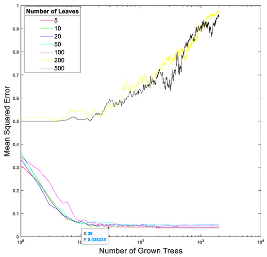
Figure 15.
The relationship between the mean squares error and the total number of trees at different total numbers of leaf nodes in the random forest in our proposed method trained using the EEGs acquired from Hejian performing the reading activity under the concentration state on the first day.
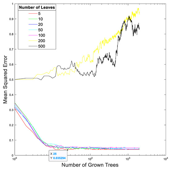
Figure 16.
The relationship between the mean squares error and the total number of trees at different total numbers of leaf nodes in the random forest in our proposed method trained using the EEGs acquired from Hejian performing the reading activity under the concentration state on the second day.
Table 12 shows the optimal parameters in the SVM in our proposed method trained using the EEGs acquired from Hejian performing the reading activity under the concentration state on both the first day and the second day. Here, the parameters to be investigated are the value of the box constraint, the type of the kernel functions, and the parameter in the kernel function. It can be seen from Table 11 that the optimal parameters in the SVM in our proposed method trained using the EEGs acquired on the first day are very different from those acquired on the second day.
Table 12.
The optimal parameters in the SVM in our proposed method trained using the EEGs acquired from Hejian performing the reading activity under the concentration state on both the first day and the second day.
Figure 17 shows the percentages of the classification accuracies yielded by our proposed method with three different classifiers trained using the EEGs acquired from Hejian performing the reading activity under the concentration state on both the first day and the second day. It can be seen that the percentages of the classification accuracies trained using the EEGs acquired on the first day are similar to those trained on the second day for all three classifiers. Hence, the dates of the measurements can be ignored for performing the classification.
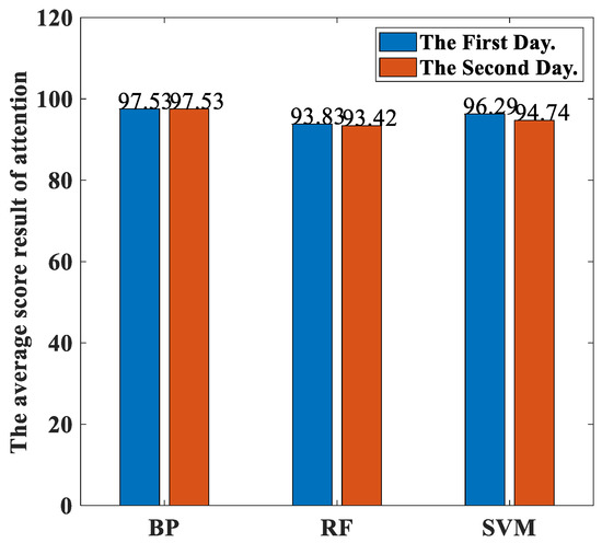
Figure 17.
The percentages of the classification accuracies yielded by our proposed method with three different classifiers trained using the EEGs acquired from Hejian performing the reading activity under the concentration state on both the first day and the second day.
5. Conclusions
The advantage of our proposed method is the ability to perform a subjective and effective attention assessment of the participants when conducting various activities. In particular, this paper proposes a classification method for performing the regression task so that it is not required to have reference values from medical officers. First, FFT is employed for performing denoising. Then, EMD is applied to remove the underlying trend. Next, SSA is employed to increase the total number of components for performing feature extraction. After that, three different types of classifiers, namely the random forest-based classifier, the SVM-based classifier, and the BP neural network-based classifier, are employed for performing the classification. Finally, the percentages of the classification accuracies are employed as the score for concentration or for immersion. The computer numerical simulation results show that the average percentages of the classification accuracies over both 12 participants and over three classifiers yielded by our proposed method are higher than those yielded by the traditional methods for all the activities as well as for both the concentration state and the immersion state. Moreover, it is found that the highest score recorded in the concentration state yielded by our method is 100. This demonstrates that our proposed method yields a better classification performance. In addition, there are similar sorting orders of the activities yielded by both our proposed method and the traditional methods for both the concentration state and the immersion state. This demonstrates that our proposed method is reliable. Furthermore, as it is required to pay more attention when performing the reading activity and the doing computer exercise activity compared to performing the eating activity and the playing toy activity, our obtained results are consistent with this result. Hence, our obtained results are reasonable. Moreover, it is found that it is not necessarily true for the average percentages of the classification accuracies over both these 12 participants and over these three classifiers for performing the various activities yielded by both our proposed method and the traditional methods under the concentration state to be higher than those under the immersion state. Finally, it is found that the random forest-based classifier yields the highest average percentages of the classification accuracies compared to the SVM-based classifier and the BP neural network-based classifier for both the concentration state and the immersion state as well as for both our proposed method and the traditional method.
The limitation of our proposed method is the hardware constraint. Here, only a single-channel EEG device is employed for performing the data acquisition. Hence, the information that can be extracted from the EEGs is limited. To address this issue, more types of signals such as image sequences and motion signals will be used in the future for performing the attention assessment. In particular, a camera and a motion sensor will be employed for acquiring the data. Then, the new set of features extracted from the image sequences and the motion signals will be added to the existing features extracted from the single-channel EEGs. At present, only a small amount of EEGs is acquired. That is why the percentages of the classification accuracies of some cases are 100. In the future, more measurements will be obtained. Hence, the percentages of the classification accuracies will be more reliable.
Author Contributions
Conceptualization, W.W. and B.W.-K.L.; methodology, W.W. and B.W.-K.L.; software, W.W.; validation, R.L., Z.L., Q.L. and J.S.; formal analysis, W.W. and B.W.-K.L.; investigation, W.W. and B.W.-K.L.; resources, C.Y.-F.H.; data curation, C.Y.-F.H.; writing—original draft preparation, W.W.; writing—review and editing, W.W. and B.W.-K.L.; visualization, W.W.; supervision, B.W.-K.L.; project administration, B.W.-K.L.; funding acquisition, B.W.-K.L. All authors have read and agreed to the published version of the manuscript.
Funding
This paper was supported partly by the National Nature Science Foundation of China (no. U1701266, no. 61671163, no. 62071128 and no. 61901123), the Team Project of the Education Ministry of the Guangdong Province (no. 2017KCXTD011), the Guangdong Higher Education Engineering Technology Research Center for Big Data on Manufacturing Knowledge Patent (no. 501130144), and the Hong Kong Innovation and Technology Commission, Enterprise Support Scheme (no. S/E/070/17).
Institutional Review Board Statement
Not applicable.
Informed Consent Statement
Informed consent was obtained from all subjects involved in the study.
Data Availability Statement
The data will be provided based on the request manner.
Conflicts of Interest
The authors declare that there is no conflict of interest.
References
- Mohammadpour, M.; Mozaffari, S. Classification of EEG-Based Attention for Brain Computer Interface. In Proceedings of the 2017 3rd lranian Conference on Intelligent Systems and Signal Processing, Shahrood, Iran, 20–21 December 2017; pp. 34–37. [Google Scholar]
- Pai, W.; Mei, W.; Fan, W.; Xue-Bin, Q. Research on Attention Classification Based on Long Short-term Memory Network. In Proceedings of the 2020 5th International Conference on Mechanical, Control and Computer Engineering, Harbin, China, 25–27 December 2020; pp. 1152–1155. [Google Scholar]
- Teplan, M. Fundamentals of EEG measurement. Meas. Sci. Rev. 2002, 2, 1–11. [Google Scholar]
- Ray, W.J.; Cole, H.W. EEG alpha activity reflects attentional demands and beta activity reflects emotional and cognitive processes. Science 1985, 228, 750–752. [Google Scholar] [CrossRef] [PubMed]
- Schacter, D.L. EEG theta waves and psychological phenomena: A review and analysis. Biol. Psychol. 1977, 5, 47–82. [Google Scholar] [CrossRef] [PubMed]
- Harmony, T.; Fernández, T.; Silva, J.; Bernal, J.; Díaz-Comas, L.; Reyes, A.; Marosi, E.; Rodriguez, M.; Rodriguez, M. EEG delta activity: An indicator of attention to internal processing during performance of mental tasks. Int. J. Psychophysiol. 1996, 24, 161–171. [Google Scholar] [CrossRef]
- Wolpaw, J.R.; Birbaumer, N.; McFarland, D.J.; Pfurtscheller, G.; Vaughan, T.M. Brain–computer interfaces for communication and control. Clin. Neurophysiol. 2002, 113, 767–791. [Google Scholar] [CrossRef]
- Zhao, G.; Ge, Y.; Shen, B.; Wei, X.; Wang, H. Emotion Analysis for Personality Inference from EEG Signals. IEEE Trans. Affect. Comput. 2018, 9, 362–371. [Google Scholar] [CrossRef]
- Huang, Z.; Ling, B.W.-K. Sleeping stage classification based on joint quaternion valued singular spectrum analysis and ensemble empirical mode decomposition. Biomed. Signal Process. Control 2002, 71, 103086. [Google Scholar] [CrossRef]
- Delisle-Rodriguez, D.; Villa-Parra, A.C.; Bastos-Filho, T.; López-Delis, A.; Frizera-Neto, A.; Krishnan, S.; Rocon, E. Adaptive Spatial Filter Based on Similarity Indices to Preserve the Neural Information on EEG Signals during On-Line Processing. Sensors 2017, 17, 2725. [Google Scholar] [CrossRef]
- Liu, Y.; Li, M.; Zhang, H.; Wang, H.; Li, J.; Jia, J.; Wu, Y.; Zhang, L. A tensor-based scheme for stroke patients’ motor imagery EEG analysis in BCI-FES rehabilitation training. J. Neurosci. Methods 2014, 222, 238–249. [Google Scholar] [CrossRef]
- Shenjie, S.; Thomas, K.P.; Smitha, K.G.; Vinod, A.P. Two player EEG-based neurofeedback ball game for attention enhancement. In Proceedings of the 2014 IEEE International Conference on Systems, Man, and Cybernetics (SMC), San Diego, CA, USA, 5–8 October 2014; pp. 3150–3155. [Google Scholar]
- Khong, A.; Jiangnan, L.; Thomas, K.; Vinod, A.P. BCI based multi-player 3-D game control using EEG for enhancing attention and memory. In Proceedings of the 2014 IEEE International Conference on Systems, Man, and Cybernetics (SMC), San Diego, CA, USA, 5–8 October 2014; pp. 1847–1852. [Google Scholar]
- Mohammadi, S.; Enshaeifar, S.; Ghavami, M.; Sanei, S. Classification of awake, REM and NREM from EEG via singular spectrum analysis. In Proceedings of the 2015 37th Annual International Conference of the IEEE Engineering in Medicine and Biology Society, Milano, Italy, 25–29 August 2015; pp. 4769–4772. [Google Scholar]
- Mohammadi, S.; Kouchaki, S.; Ghavami, M.; Sanei, S. Improving time-frequency domain sleep EEG classification via singular spectrum analysis. J. Neurosci. Methods 2016, 273, 96–106. [Google Scholar] [CrossRef]
- Maddirala, A.; Shaik, R. Motion artifact removal from single channel electroencephalogram signals using singular spectrum analysis. Biomed. Signal Process. Control 2016, 30, 79–85. [Google Scholar] [CrossRef]
- Maddirala, A.; Shaik, R. Removal of EOG Artifacts from single channel EEG signals using combined singular spectrum analysis and adaptive noise canceler. IEEE Sens. J. 2016, 16, 8279–8287. [Google Scholar] [CrossRef]
- Ayain, S.; Saraoglu, H.; Kara, S. Singular Spectrum Analysis of Sleep EEG in Insomnia. J. Med. Syst. 2011, 35, 457–461. [Google Scholar]
- Golyandina, N.; Nekrutkin, V.; Zhigljavsky, A.A. Analysis of Time Series Structure: SSA and Related Techniques; CRC/Chapman & Hall: New York, NY, USA, 2001. [Google Scholar]
- Hassani, H. Singular spectrum analysis: Methodology and comparison. J. Data Sci. 2007, 5, 239–257. [Google Scholar] [CrossRef] [PubMed]
- Vijayasankar, A.; Kumar, P.R. Correction of blink artifacts from single channel EEG by EMD-IMF thresholding. In Proceedings of the 2018 Conference on Signal Processing and Communication Engineering Systems (SPACES), Vijayawada, India, 4–5 January 2018; pp. 176–180. [Google Scholar]
- Khare, S.K.; Gaikwad, N.B.; Bajaj, V. VHERS: A Novel Variational Mode Decomposition and Hilbert Transform-Based EEG Rhythm Separation for Automatic ADHD Detection. IEEE Trans. Instrum. Meas. 2022, 71, 1–10. [Google Scholar] [CrossRef]
- Mohguen, W.; El’hadi Bekka, R. Comparative Study of ECG Signal Denoising by Empirical Mode Decomposition and Thresholding Functions. In Proceedings of the 2019 6th International Conference on Electrical and Electronics Engineering (ICEEE), Istanbul, Turkey, 16–17 April 2019; pp. 126–130. [Google Scholar]
- Lin, P.; Kuang, W.; Liu, Y.; Ling, B.W.-K. Grouping and selecting singular spectrum analysis components for denoising via empirical mode decomposition approach. Circuits Syst. Signal Process. 2019, 38, 356–370. [Google Scholar] [CrossRef]
- Srinivasan, V.; Eswaran, C.; Sriraam, N. Approximate Entropy-Based Epileptic EEG Detection Using Artificial Neural Networks. IEEE Trans. Inf. Technol. Biomed. 2007, 11, 288–295. [Google Scholar] [CrossRef]
- Hu, L.; Zhao, K.; Zhou, X.; Ling, B.W.-K.; Liao, G. Empirical Mode Decomposition Based Multi-Modal Activity Recognition. Sensors 2020, 20, 6055. [Google Scholar] [CrossRef]
- Li, H. Network traffic prediction of the optimized BP neural network based on Glowworm Swarm Algorithm. Syst. Sci. Control. Eng. 2019, 7, 64–70. [Google Scholar] [CrossRef]
- Yang, X.; Yu, Q.; He, L.; Guo, T. The one-against-all partition based binary tree support vector machine algorithms for multi-class classification. Neurocomputing 2013, 113, 1–7. [Google Scholar] [CrossRef]
- Minasyan, G.R.; Chatten, J.B.; Harner, R.N. Detection of epileptiform activity in unresponsive patients using ANN. In Proceedings of the 2009 International Joint Conference on Neural Networks, Atlanta, GA, USA, 14–19 June 2009; pp. 2117–2124. [Google Scholar]
- AIa, K.; Byeon, J.G.; Timashev, S.F.; Vstovskiĭ, G.V.; Park, B.W. Functional variability of the autocorrelation structure of the EEG. Zhurnal Vyss. Nervn. Deiatelnosti Im. IP Pavlov. 2006, 56, 408–411. [Google Scholar]


Disclaimer/Publisher’s Note: The statements, opinions and data contained in all publications are solely those of the individual author(s) and contributor(s) and not of MDPI and/or the editor(s). MDPI and/or the editor(s) disclaim responsibility for any injury to people or property resulting from any ideas, methods, instructions or products referred to in the content. |
© 2023 by the authors. Licensee MDPI, Basel, Switzerland. This article is an open access article distributed under the terms and conditions of the Creative Commons Attribution (CC BY) license (https://creativecommons.org/licenses/by/4.0/).