Abstract
Batch process monitoring datasets usually contain missing data, which decreases the performance of data-driven modeling for fault identification and optimal control. Many methods have been proposed to impute missing data; however, they do not fulfill the need for data quality, especially in sensor datasets with different types of missing data. We propose a hybrid missing data imputation method for batch process monitoring datasets with multi-type missing data. In this method, the missing data is first classified into five categories based on the continuous missing duration and the number of variables missing simultaneously. Then, different categories of missing data are step-by-step imputed considering their unique characteristics. A combination of three single-dimensional interpolation models is employed to impute transient isolated missing values. An iterative imputation based on a multivariate regression model is designed for imputing long-term missing variables, and a combination model based on single-dimensional interpolation and multivariate regression is proposed for imputing short-term missing variables. The Long Short-Term Memory (LSTM) model is utilized to impute both short-term and long-term missing samples. Finally, a series of experiments for different categories of missing data were conducted based on a real-world batch process monitoring dataset. The results demonstrate that the proposed method achieves higher imputation accuracy than other comparative methods.
1. Introduction
The batch process is an important production mode in the modern manufacturing industry. As a highly flexible production method, the batch process is essential in producing low-volume, high-value-added products, such as chemical and biological materials [1,2]. With the rapid development of the Internet of Things and sensing technology [3], the monitoring data of batch processes is being recorded more frequently. However, batch process monitoring data often contains missing values due to factors such as external environmental conditions, link failures, and sensor equipment degradation. This results in incomplete and unreliable batch process monitoring data, which poses a significant obstacle to the subsequent utilization of the data [4]. Especially, missing data will decrease the performance of data-driven modeling for fault identification and optimal control in batch processes. Therefore, it is significant to study how to deal with missing data to enhance the quality of batch process monitoring data.
There are mainly two categories of methods to handle missing data: deletion and imputation [5,6]. The deletion method may not only lose valuable information within the data but also destroy the continuity of the time series, leading to inaccurate results in subsequent data analysis. The imputation method involves replacing missing values with predicted values [7], which is more suitable for improving data quality. However, there are few studies that focus on missing data imputation for batch process monitoring datasets. Nomikos et al. [8] employed the mean method for imputing missing values. Laila et al. [9] and Meng et al. [10] introduced a methodology where the unknown observations are calculated using a weighted combination of scores from the current time point in the new batch and previously computed scores from a calibration dataset. Shi et al. [11] established a linear regression model that uses several historical values adjacent to the current time to predict the missing values. Further research is needed, as the imputation results of these methods have shown limited effectiveness.
Due to the characteristics of batch processes, such as multiple operating conditions, multiple batches, and multiple stages, missing data in batch process monitoring datasets usually presents a complex situation, making it challenging to perform accurate imputation. Furthermore, batch process monitoring datasets contain different types of missing data and directly applying an existing single method cannot achieve favorable imputation results. Consequently, how to combine or improve appropriate imputation models to effectively impute missing data within batch process monitoring datasets is still a significant problem to be solved.
In this paper, we propose a hybrid missing data imputation method for batch process monitoring datasets based on single-dimensional interpolation, a multivariate regression model, and LSTM. The main contributions are as follows:
- We propose a missing data classification method based on the continuous missing duration for each variable and the number of variables missing simultaneously. Then we classify the missing data into five distinct categories: transient isolated missing values, short-term missing variables, long-term missing variables, short-term missing samples, and long-term missing samples.
- We design and implement the hybrid missing data imputation method to deal with different categories of missing data step by step, taking into account the characteristics of different categories of missing data. This method employs a combination of three single-dimensional interpolation models that enables the automated detection and imputation of transient isolated missing values. We design an iterative imputation based on a multivariate regression model to automatically complete the imputation of all long-term missing variables. To address short-term missing variables, we propose a combination model based on single-dimensional interpolation and multivariate regression by utilizing system fluctuations. We use the LSTM model to impute both short-term and long-term missing samples.
- We have carried out extensive experiments on a real-world injection molding process monitoring dataset to demonstrate the effectiveness and accuracy of the proposed hybrid missing data imputation method.
The remainder of this paper is structured as follows. Section 2 presents the related works. Section 3 describes the hybrid missing data imputation method designed. Section 4 verifies the validity of the proposed method by taking a real-world injection molding process monitoring dataset as an example. Section 5 presents the conclusions.
2. Related Works
Many imputation techniques have been proposed for different domain-specific datasets [12], primarily involving two categories: statistical and machine learning-based techniques [13,14].
Statistical imputation techniques rely on statistical models to predict missing values. Simple imputation handles missing values by using methods such as the mode, mean, or median of the available values [15]. Hot-deck imputation handles missing values by replacing them with similar object values [16]. Interpolation methods, which mainly include nearest neighbor interpolation, linear interpolation, and spline interpolation, estimate missing values by establishing interpolation functions [17]. These techniques perform imputation based on temporal continuity and are effective in the case of a handful of missing values. Regression imputation involves estimating relationships among variables using regression modeling [18], which typically includes Linear Regression (LR) and Multivariate Linear Regression (MLR). This approach can effectively utilize the correlations between time series data for imputation. Matrix-based methods recover missing data by treating an entire set of series as a matrix and applying techniques based on matrix completion principles [19]. These techniques leverage temporal continuity for imputation and mainly include Singular Value Decomposition (SVD), Principal Component Analysis (PCA), Matrix Factorization (MF), and Centroid Decomposition (CD)-based methods. PCA-based methods, SPIRIT [20] and ROSL [21], are effective for datasets with a limited number of time series or short time series. SVD-based SoftImpute [22] and MF-based TRMF [23] require data to contain repeating trends, while CD-based CDRec [24] is only effective for correlated time series. Pattern-based methods utilize pattern-matching techniques for imputation by leveraging trend similarity. For instance, STMVL [25] derives statistical models from historical data and requires highly correlated time series. DynaMMo [26] employs Kalman filters and Expectation-Maximization (EM) for imputation and is adaptable to datasets with irregular fluctuations.
Machine learning techniques are widely used in various practical application fields, such as air pollution monitoring [27], industrial process monitoring [2], dam safety monitoring [28,29], medical data processing [30], and stock price prediction [31]. To address the challenges posed by missing data, several machine learning-based methods have gained significant popularity [12]. The K Nearest Neighbor (KNN) algorithm [32] works by classifying the nearest neighbors of missing values and using those neighbors for imputation through a distance measure between instances. The Random Forest (RF) algorithm [33,34] constructs multiple decision trees based on the bootstrapping procedure and gives the final predictions by the averaged values or majority votes of each tree’s prediction. The K-means clustering algorithm [35] consists of 2 steps, where the first step gets clusters using K-means clustering, and then the second step handles missing values using cluster information. These methods utilize the correlation between time series but do not consider the continuity in the time dimension. And more advanced neural networks have also been applied to deal with missing values in time series data. The Extreme Learning Machine (ELM) [36] is an efficient machine learning model based on a single-layer feedforward neural network and is suitable for multi-dimensional time series with multiple features. Long Short-Term Memory (LSTM) [37], which is an improved form of Recurrent Neural Networks (RNNs) [38], can effectively learn long-term dependencies for predicting multi-dimensional time series.
In summary, although several imputation methods have been proposed, most of them are typically designed to estimate a specific type of missing data. And these methods often excel only when handling datasets with specific data characteristics. In practical domains, such as batch process monitoring datasets, missing data usually presents a complex situation. These datasets contain different types of missing data, and different types of missing data exhibit distinct characteristics. Applying a single imputation method directly may not be effective. Therefore, further research is still needed on how to conduct classification analysis of missing data and design a hybrid method by employing suitable imputation techniques tailored to the characteristics of different types of missing data.
3. Methodology
3.1. Data Processing
3.1.1. Data Unfolding
For a typical batch process, the monitoring data is stored in a three-dimensional matrix, , where I represents the number of batches, J represents the number of process variables, and T represents the number of sampling moments in a batch. Since subsequent research on missing data imputation involves analyzing and processing missing variables at different sampling moments, it is necessary to unfold the original three-dimensional data along the batch dimension to obtain two-dimensional data, that is, of batches. As shown in Figure 1, I matrix slices are obtained by unfolding the original three-dimensional data along the batch dimension. Each matrix slice represents a set of values for variable at sampling moments .

Figure 1.
Unfolding data along the batch dimension.
3.1.2. Missing Data Classifying
The assumption in this paper is to impute missing data based on dataset denoising. The missing data can arise from data acquisition as well as from data denoising. Regarding the missing data caused by data acquisition, the causes of missing data in batch process monitoring can be summarized into the following three cases: (1) Production equipment outage, acquisition system failures, or data link failures lead to long or short periods of continuous missing for many variables; (2) Acquisition equipment failures lead to long or short periods of continuous missing for a few variables; (3) The instability or aging of acquisition equipment leads to isolated missing values for a few variables.
Based on the cause analysis of missing data, the classification rules for missing data are defined, as shown in Table 1. represents the continuous missing duration of a variable, represents the number of variables missing simultaneously during this period. represents the data sampling interval, represents the time threshold at which the data trend does not change, represents the time threshold at which the data trend can be predicted. and are set according to the specific situation of different variables and the practical requirements for data analysis. Variable threshold represents the critical value for the number of variables missing simultaneously in a certain period (longer than ), and is set to , where n represents the number of variables in batch process monitoring dataset.

Table 1.
Classification rules for missing data in batch process monitoring dataset.
By calculating the continuous missing duration for each variable and the corresponding number of variables missing simultaneously, and then comparing the calculated results with the threshold values, the missing data is classified into five categories: transient isolated missing values, short-term missing variables, long-term missing variables, short-term missing samples, and long-term missing samples. Short-term and long-term missing variables are categorized as continuous missing variables, while short-term and long-term missing samples are categorized as continuous missing samples. Variables without any missing values are referred to as complete variables, while variables with missing values are referred to as incomplete variables.
3.2. Missing Data Imputation
3.2.1. Dataset Splitting
Due to the presence of many incomplete variables within the continuous missing samples, it can be considered that a system outage occurred during this period. The data segment with continuous missing samples can be seen as a missing data segment. Therefore, the unfolded dataset needs to be split into several data segments according to the locations of continuous missing samples and then imputed. Assuming that the dataset X is split times, then the dataset X contains K data segments and missing data segments (data segments with short-term or long-term missing samples):
where represent the k-th data segment, and each data segment contains only transient isolated missing values, short-term or long-term missing variables, represent the missing data segment between the k-th and (k + 1)-th data segments.
Variable Missing Proportion (VMP) and Sample Missing Proportion (SMP) are introduced as measures to describe the extent of missing data within each data segment. Taking data segment as an example, the sample missing proportion of and the variable missing proportion of variable in are calculated as follows:
where is the sample size of , n is the number of variables in , represents the sample size without missing values, and represents the number of values that are not missing in variable j.
3.2.2. Transient Isolated Missing Values Imputation
For transient isolated missing values, the data trend in the time dimension remains unchanged. The missing values can be estimated using single-dimensional interpolation models based on temporal continuity. The nearest neighbor interpolation, linear interpolation and cubic spline interpolation are used. Assuming that (the i-th value of variable j) in data segment is missing, and represents the estimated value of .
(1) Single-dimensional Interpolation Model
The nearest neighbor interpolation: The interpolation function is established using a valid value adjacent to , as shown in Formula (3). The limitation of this method is the discontinuity at .
The linear interpolation: The interpolation function is constructed using two valid value adjacent to , as shown in Formula (4). While linear interpolation ensures continuity at , it lacks derivability at the endpoints.
The cubic spline interpolation: The cubic spline interpolation requires at least four valid values and constructs the interpolation function using two adjacent values before and two adjacent values after , as shown in Formula (5). The detailed construction process can be found in reference [39].
When both values and are missing simultaneously ( is set to 2), the interpolation Formulas (3), (4), and (5) need to be reconstructed, respectively, as shown in Formulas (6)–(8).
where is the interpolated value of , and , respectively, represent the cubic spline interpolation functions for and .
(2) Imputation Process for Transient Isolated Missing Values
To impute the transient isolated missing values in the data segment , a combination of the above three interpolation models is employed. Combining these three methods enables the automated detection and imputation of transient isolated missing values, making it an efficient complementary approach. When four adjacent valid values are available, cubic spline interpolation is utilized for imputation. If the four adjacent values do not consist of two values before and two values after , the cubic spline interpolation function needs to be adjusted. Taking one value before and three values after as an example, the adjusted cubic spline interpolation function is shown in Formula (9).
When the missing value is located at the endpoint of , meaning that only one side (either left or right) has an adjacent value, the nearest neighbor interpolation is utilized for imputation. When two adjacent valid values are available, with one before and one after , the linear interpolation is used for imputation.
3.2.3. Continuous Missing Variables Imputation
In the case of a long-term missing variable, significant information in the time dimension is seriously lost. The missing values of the long-term missing variable can only be estimated based on the correlation with other complete variables. The multivariate regression model is suitable for imputing missing values for long-term missing variables. The model constructs a regression function between the long-term missing variable and other complete variables based on their correlations. Then, by utilizing the complete variables as input, the missing values of the long-term missing variable can be predicted. In the case of a short-term missing variable, the missing values can be estimated by considering the correlation with other complete variables, together with the data trend in the time dimension. Therefore, a combination model based on single-dimensional interpolation and multivariate regression is proposed to impute the missing values of short-term missing variables by combining the strengths of both models.
(1) Multivariate Regression Model
Three widely used multivariate regression models are chosen for this study: MLR, RF, and KNN. All three models exhibit robustness and require minimal or no parameters. Assuming that and are the input and output of training data, respectively, and and are the input and output of testing data, respectively, where represents the sample size of the training data, n represents the number of variables, represents the sample size of the testing data.
MLR establishes a linear regression function by considering the correlation between the incomplete variable and other complete variables. Then, the function is utilized to predict the missing values. An advantage of the MLR model is its lack of reliance on hyperparameters. The missing values imputation process using MLR is as follows:
Step 1: Modeling. Construct the MLR function:
where is the design matrix for and , is a constant vector, is the error vector, is the coefficient vector, can be estimated by Formula (11):
where is the estimated value of , is the transpose matrix of , is the inverse matrix of and .
Step 2: Missing values prediction. Estimate using :
where is the design matrix for and , is a constant vector.
RF is an ensemble learning model based on the Classification and Regression Tree (CART). The RF model requires two hyperparameters and , which respectively represent the number of trees and the number of selected features. The missing value imputation process using the RF model is as follows:
Step 1: RF model training.
Step 1.1: Utilize the Bootstrap resampling method to select samples from the original training dataset with replacement, and remove duplicate samples to create a new training dataset .
Step 1.2: Train CART decision trees using dataset to generate the trained CART model . During the training process, randomly select features from all the features, and then identify the optimal feature within the selected features as the splitting point for partitioning each node into left and right segments.
Step 1.3: Repeat Steps 1.1–1.2 times to obtain CART decision trees, denoted as the prediction model .
Step 2: Missing values prediction.
Step 2.1: Select the same features as used in the training process to create a new testing dataset .
Step 2.2: Input into the trained model to obtain the first prediction result .
Step 2.3: Repeat Steps 2.1–2.2 until obtaining prediction results.
Step 2.4: Calculate the final prediction result using the mean method:
The KNN regression model involves considering three factors [40]: the number of nearest samples (k), the distance measurement method, and the regression prediction rule. The distance measurement method employs the widely used Euclidean distance, while the regression prediction rule is based on the mean method. The appropriate value for k can be determined through cross-validation based on the sample distribution. The missing value imputation process using KNN is outlined below.
Step 1: Calculate the Euclidean distance between the s-th sample in and the t-th sample in , as shown in Formula (14). Then, calculate the distance between and all the samples in to obtain the distance vector .
where is the s-th sample in , is the t-th sample in , n is the number of variables.
Step 2: Choose k nearest samples in according to the k smallest values in the distance vector .
Step 3: Calculate the average of the values in that correspond to these k nearest samples, as shown in Formula (15), and set this average value as the predicted value for the sample .
Step 4: Repeat steps 1–3 to calculate predicted values for all samples in , then all values in are obtained.
(2) Imputation Process for Long-term Missing Variables
Since the multivariate regression model has the limitation that only one variable can be imputed in each process, an iterative method is designed to overcome this constraint. The iterative imputation based on the multivariate regression model can automatically complete the imputation of all long-term missing variables. The model from MLR, RF, or KNN is selected as multivariate regression model . Assuming that is the data segment after imputing transient isolated missing values, and is the number of long-term missing variables in . The iterative imputation based on a multivariate regression model is presented in Algorithm 1.
| Algorithm 1 The iterative imputation based on multivariate regression model |
| Input: , |
| Output: The imputed data segment |
| 1. Begin |
|
| 3. Set ; |
| 4. For to : |
|
|
|
| 8. Impute using ; |
| 9. Set ; |
| 10. Return ; |
| 11. End |
(3) Imputation Process for Short-term Missing Variables
The combination model based on single-dimensional interpolation and multivariate regression is developed for imputing the missing values of short-term missing variables. This combination model is based on the property that a missing variable experiences system fluctuations due to the influence of its related variables. The model utilizes a multivariate regression model to calculate the system fluctuation and incorporate it into the interpolation value. By considering the continuity in the time dimension and the correlation among different variables, this model significantly enhances imputation accuracy by combining the strengths of both models.
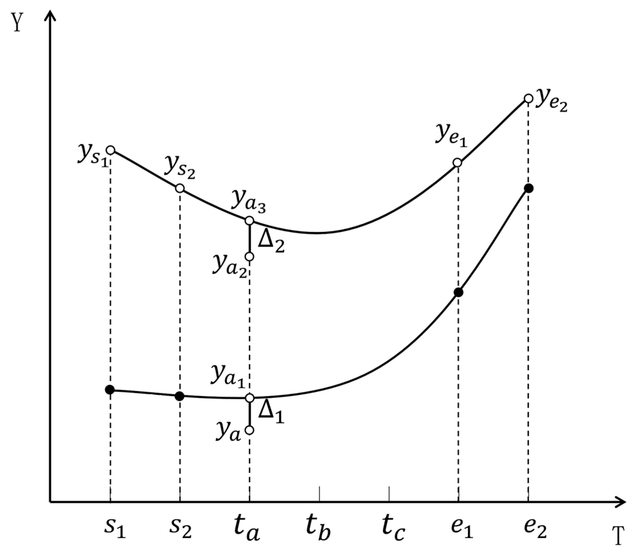
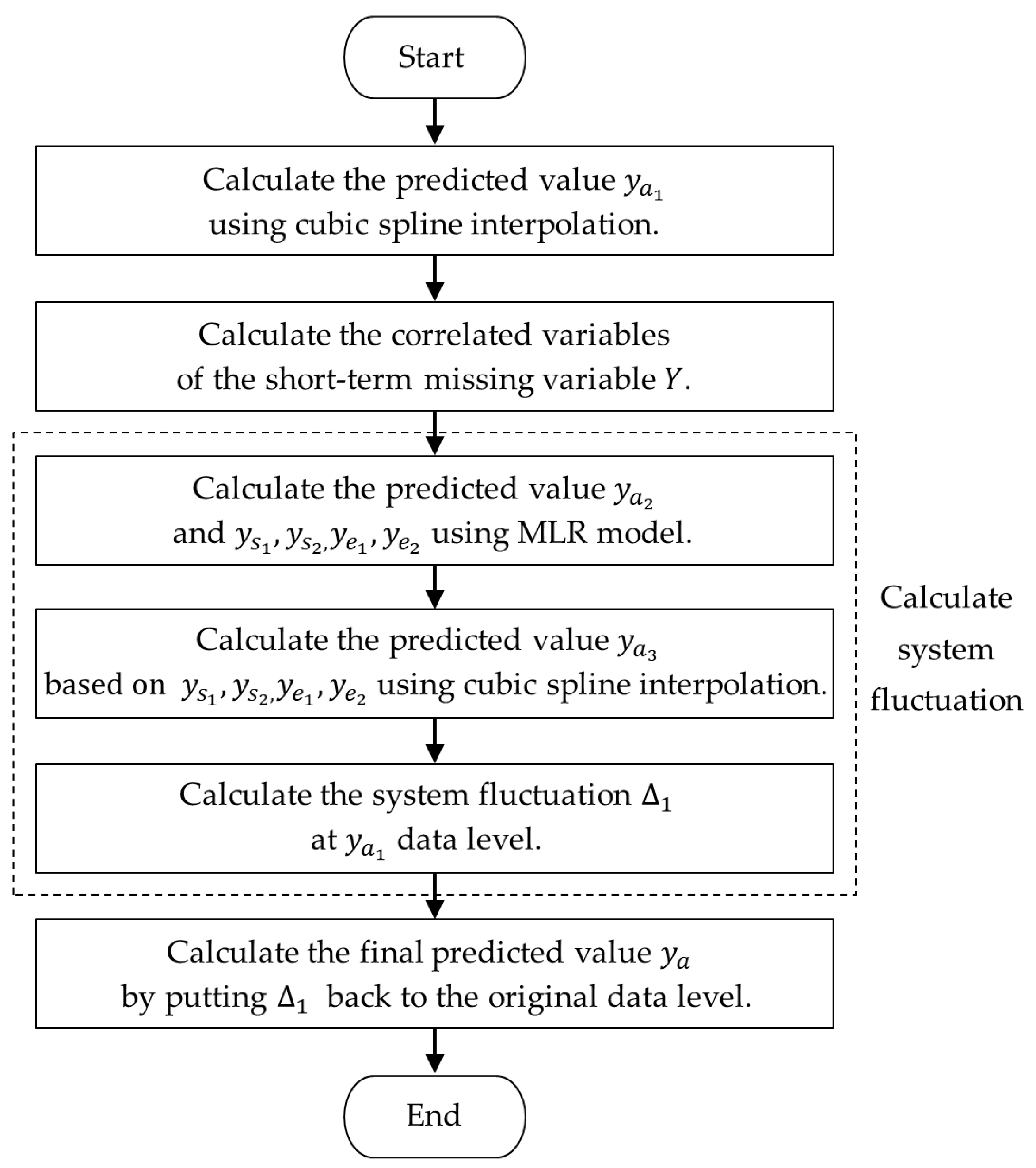
Taking cubic spline interpolation and MLR as examples, the combination model for imputing missing values of short-term missing variables is designed. As shown in Figure 2, variable in data segment contains short-term missing from time to time . and , respectively, represent the corresponding time with a valid value on the left side of and on the right side of . The continuous missing duration , and . Time represent three sampling times in this period. represents the predicted value at time , the imputation process for based on the combination model is shown in Figure 3.
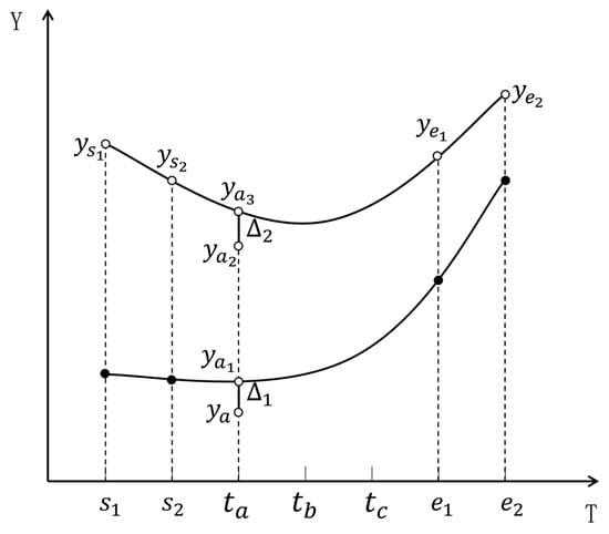
Figure 2.
Example of short-term missing variable imputation based on the combination model.

Figure 3.
Imputation process for short-term missing variable based on the combination model.
Step 1: Calculate the predicted value at time using cubic spline interpolation by Formula (8).
Step 2: Calculate the correlation between variable and the short-term missing variable using Formula (16). If , variable is the correlated variable with . Then identify all the correlated variables with , denoted as .
where , is the sample size, is the correlation threshold, is the number of correlated variables with .
Step 3: The variable is influenced by its correlated variables, which leads to system fluctuations. The MLR model and cubic spline interpolation are used to calculate the system fluctuation at data level:
Firstly, use the MLR model for regression fitting to describe the relationship between and its correlated variables, and the corresponding predicted values at time are calculated by Formula (12), where the dataset formed by all the correlated variables is used as the testing data, is the sample size of , and the sample size of in Formula (12) is set to .
Then construct a cubic spline interpolation function based on values by Formula (8), and get the predicted value at time .
Finally, calculate the system fluctuation at data level by Formula (17). Since the system fluctuation is influenced by the data level, the relationship between and satisfies Formula (18). So the system fluctuation is calculated by Formula (19).
Step 4: Put the system fluctuation back to the original data level, as shown in Formula (20), and then the final predicted value at time is calculated:
3.2.4. Continuous Missing Samples Imputation
After data splitting, the information between data segments is not only lost in time dimension but also among different variables. It is difficult to impute short-term and long-term missing samples using a single-dimensional interpolation model or a multivariate regression model. We adopt the LSTM model, which can effectively learn long-term dependencies, to impute continuous missing samples after imputing transient isolated missing values and continuous missing variables.
(1) LSTM Model
The 5-layer LSTM network for the prediction of missing values in continuous missing samples is as below.
Input layer: This layer receives input data, where the number of variables in the input data is consistent with the number of neurons in this layer.
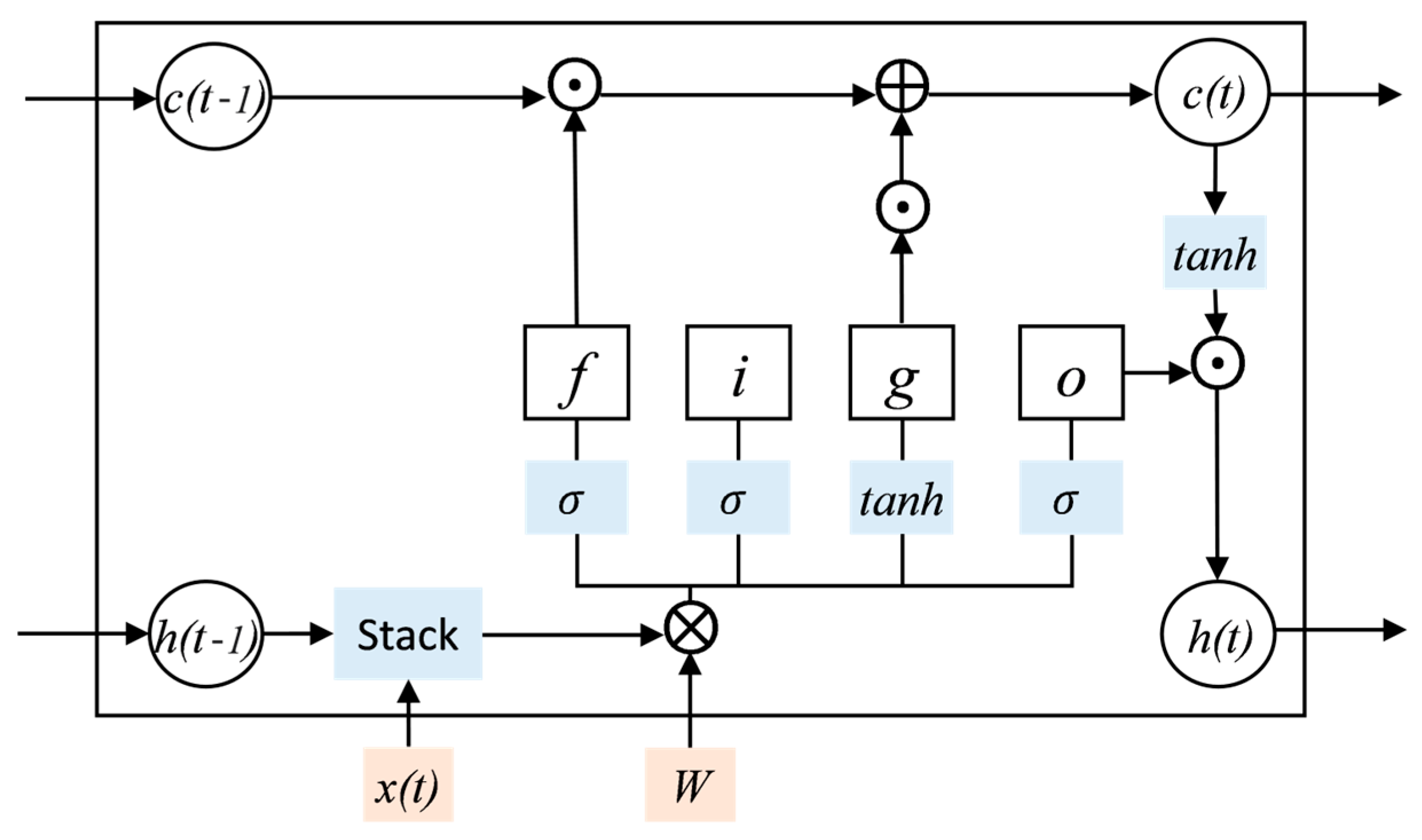
LSTM layer: This layer builds the LSTM model. The LSTM unit structure is shown in Figure 4. The memory unit in LSTM has four gates: INPUT GATE (), FORGET GATE (), UPDATE GATE (), and OUTPUT GATE (). is the unit state, representing the information learned before time , which can be seen as long-term memory. is the hidden state, representing the output of the network in the current state, which can be seen as short-term memory. is the current time network input value. The forget gate determines the retention degree of the current state to the cell state at the previous moment. The input gate determines the retention degree of the current state to the input . The output gate controls the degree to which outputs to in the current state. Each node in the LSTM model can be calculated as below:
where f is the forget gate, i is the input gate, g is the update gate, o is the output gate, c is the unit state, h is the hidden state, σ is the activation function of Sigmoid, W is the weight matrix, b is the bias term, ⊙ represent matrix elements multiplication.
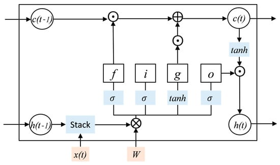
Figure 4.
LSTM unit: f is the forget gate, i is the input gate, g is the update gate, o is the output gate, c is the unit state, h is the hidden state, σ is the activation function of Sigmoid, W is the weight matrix, Stack, ⊙, ⊕ and ⊗, respectively, represent matrix stacking, matrix elements multiplication, matrix addition and matrix multiplication.
Lost layer: This layer is used to prevent overfitting [41]. During the training process, the loss probability is set to 0.5. The input data from the LSTM layer is randomly set to 0 with rate . The remaining data is scaled by the rate and then input into the fully connected layer.
Fully connected layer: This layer establishes full connection between the LSTM layer with the output layer. The number of input neurons in this layer is equal to the number of neurons in LSTM layer.
Output layer: This layer generates the prediction results. The number of output neurons is equal to the number of variables in the output data.
(2) Imputation Process for Continuous Missing Samples
The LSTM model takes all the complete data segments before the current moment as input and predicts the missing values at the current moment. Then the imputed values are used as input to predict the missing values at the next moment. Therefore, the continuous missing samples (the missing data segments) are imputed by iteratively executing the model. The iterative imputation process for the missing data segment is as follows, where mc is the sample size and n is the number of variables. And l represents the time steps (the length of input data) of the LSTM model.
Step 1: LSTM model training.
Step 1.1: Generate the training dataset based on data segment after imputing all transient isolated missing values and continuous missing variables.
Step 1.2: Initialize and train input data, where the i-th input sample of is ; then train output data, where the i-th output sample of is .
Step 1.3: Repeat Step 1.2 times.
Step 1.4: Train the LSTM model based on dataset and , then get the trained LSTM model whose output state is .
Step 2: Missing data prediction.
Step 2.1: Initialize the LSTM model, and input the training dataset into to obtain whose output state is .
Step 2.2: For , input the l consecutive samples before time t (i.e., ) into to obtain the predicted data . Then update according to Formula (23) and get .
Step 2.3: Repeat Step 2.2 until , then get the predicted data segment .
It should be noted that the input of the LSTM model is a vector, so it is necessary to reconstruct the data matrix into a vector before model training and prediction.
3.3. The Hybrid Missing Data Imputation Method
Considering the various types and high missing proportion of missing data in batch process monitoring datasets, we propose a hybrid missing data imputation method based on the above research. The method classifies missing data according to the predefined classification rules, then combines and improves a single-dimensional interpolation model, a multivariate regression model, and LSTM to step-by-step impute different categories of missing data based on their specific characteristics. The pseudocode of this hybrid method is presented in Algorithm 2.
| Algorithm 2 The proposed hybrid missing data imputation method |
| Input: The original dataset |
| Output: The imputed complete dataset |
| 1. Begin |
| 2. Unfolding data along the batch dimension, get the 2D dataset X; |
|
| 4. Splitting dataset X, get ; |
|
| 6. ← The imputed data segments; |
| 7. Standardize each data segment; |
|
| 9. ← The imputed data segments; |
|
| 11. ← The imputed data segments; |
| 12. Complete dataset ← De-standardize, and transform 2D data to 3D data; |
| 13. End |
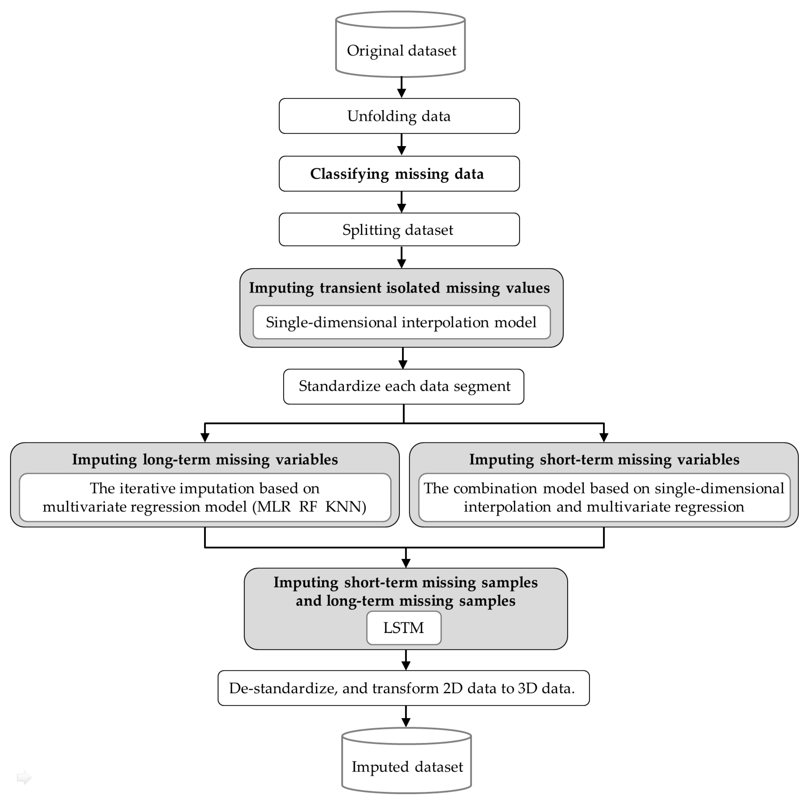
As shown in Figure 5, the proposed hybrid missing data imputation method consists of the following eight steps:
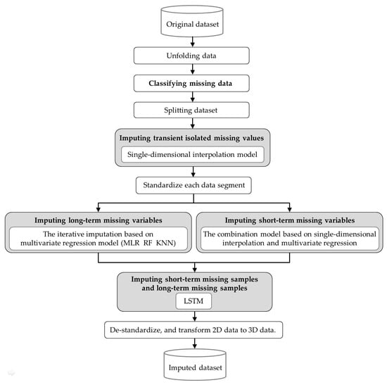
Figure 5.
The proposed hybrid missing data imputation method.
Step 1: Unfolding data: The original three-dimensional dataset is unfolded along the batch dimension to obtain two-dimensional dataset X.
Step 2: Classifying missing data: According to the missing data classification method (Section 3.1.2), the continuous missing duration for each variable and the corresponding number of variables missing simultaneously are calculated. By comparing the calculated results with the threshold values, the missing data are classified into five categories: transient isolated missing values, short-term missing variables, long-term missing variables, short-term missing samples, and long-term missing samples.
Step 3: Splitting dataset: The dataset is split according to the locations of continuous missing samples, then get , where represents the k-th data segment (the data segment with transient isolated missing values, short-term or long-term missing variables), represents the missing data segment (the data segment with short-term or long-term missing samples) between the k-th and (k + 1)-th data segments.
Step 4: Imputing transient isolated missing values: Transient isolated missing values in each data segment are imputed using three single-dimensional interpolation models as mentioned in Section 3.2.2, and the corresponding imputed data segments are .
Step 5: Standardize each data segment : Taking the variable j in data segment as an example, values are standardized using z-score standardization:
where is the standardized value of the i-th sample , is the mean of variable j, is the standard deviation of variable j, and n, respectively, represent the sample size and the number of variables in .
Step 6: Imputing long-term missing variables and short-term missing variables: For each data segment , each long-term missing variable are imputed using the iterative imputation based on multivariate regression model as mentioned in Section 3.2.3 (2), all short-term missing variables are imputed using the combination model based on single-dimensional interpolation and multivariate regression as mentioned in Section 3.2.3 (3), and the corresponding imputed data segments are .
Step 7: Imputing short-term missing samples and long-term missing samples (i.e., the missing data segments): Taking as input, all missing data segments are imputed using LSTM model as mentioned in Section 3.2.4, and the corresponding imputed data segments are .
Step 8: De-standardize the imputed data segments and transform two-dimensional data to three-dimensional data, then get the imputed complete dataset .
4. Illustration and Discussion
4.1. Data Source and Description
Injection molding, which refers to the process of making semi-finished parts of a certain shape from molten raw materials, is a typical batch process. A publicly accessible real-world injection molding dataset [42] is taken as an example, which contains data collected from both mold temperature control machines and mold sensors. Six process variables are selected, as shown in Table 2. Under this operating condition, a total of 100 normal batches with 919 sampling points are obtained, denoted as . The dataset needs to be unfolded along the batch dimension to obtain two-dimensional dataset . It includes six variables, and the length of each variable is 91,900 sampling points. The dataset contains data fluctuations, repeating trends between different batches, and dynamic correlations among different variables.

Table 2.
Process variables of a real-world injection molding process monitoring dataset.
4.2. Performance Evaluation Index
(1) Root Mean Square Error
To measure the missing data imputation accuracy, we adopt the most commonly used measure in this field: Root Mean Square Error (RMSE) [19]. The RMSE index can reflect the deviation between the predicted value and the actual value. The smaller the value of RMSE, the higher the accuracy of the algorithm. Taking variable j as an example, the RMSE value can be calculated as follows:
where is the number of missing values of variable j in data segment , is the actual value, is the predicted value of .
(2) Mean Square Error
The performance of KNN, RF, and LSTM models for missing value prediction depends on the selection of hyperparameters. We adopt Mean Square Error (MSE) to construct the loss function and utilize 10-fold cross-validation to determine the optimal hyperparameters. The smaller the value of MSE, the higher the accuracy of the algorithm. The MSE value can be calculated as follows:
where m is the sample size, n is the number of variables, is the actual value, is the predicted value of .
4.3. Data Processing
Firstly, the original three-dimensional dataset was unfolded along the batch dimension to obtain a two-dimensional dataset . According to the missing data classification rules defined in Section 3.1.2, the categories of missing data were determined. The dataset contains two data segments with continuous missing samples. Therefore, it was split into three data segments and two missing data segments according to the locations of continuous missing samples, i.e., . Data segments contain transient isolated missing values and continuous missing variables, while the two missing data segments are the data segments with continuous missing samples. In data segment , the plasticizing pressure variable contains continuous missing, while the cylinder pressure and SV2 value opening variables contain transient isolated missing values. In data segment , all variables only contain transient isolated missing values. In data segment , the plasticizing pressure variable contains continuous missing, while the nozzle temperature, cylinder pressure and SV2 value opening variables contain transient isolated missing values. The data integrity information is presented in Table 3. Considering the missing proportions of six process variables, we selected data segment with the lowest missing proportion to evaluate transient isolated missing value imputation and utilized the plasticizing pressure variable with continuous missing in data segment to evaluate continuous missing variable imputation.

Table 3.
Data integrity information.
4.4. Missing Data Imputation and Results Analysis
4.4.1. Transient Isolated Missing Values Imputation
In order to better compare the performance of different imputation methods, some transient isolated values in data segment were randomly deleted to obtain four experimental datasets with missing proportions of 5%, 10%, 15%, and 20%. The detailed imputation process for transient isolated missing values is shown in Section 3.2.2. The mean and hot-desk imputation methods were selected as baseline models.
The RMSE values for the predicted values of the six process variables calculated are shown in Table 4. Experimental results show that the single-dimensional interpolation model performs better than the mean and hot-desk imputation methods. This difference becomes more pronounced with an increasing proportion of missing values. When the missing proportion reaches 20%, the RMSE value of the single-dimensional interpolation model for the screw speed variable is 1.129, which is only about 1/3 of that obtained with the mean method.

Table 4.
RMSE of missing data imputation results for transient isolated missing values.
4.4.2. Continuous Missing Variables Imputation
To evaluate the performance of different imputation methods for imputing the continuous missing variable, the continuous missing variable (plasticizing pressure) in the data segment was imputed. The transient isolated missing values in data segment were imputed first. Methods based on single-dimensional interpolation model and a multivariate regression model were used for imputation. The detailed imputation process for the continuous missing variable is shown in Section 3.2.3.
(1) Hyperparameters Selection
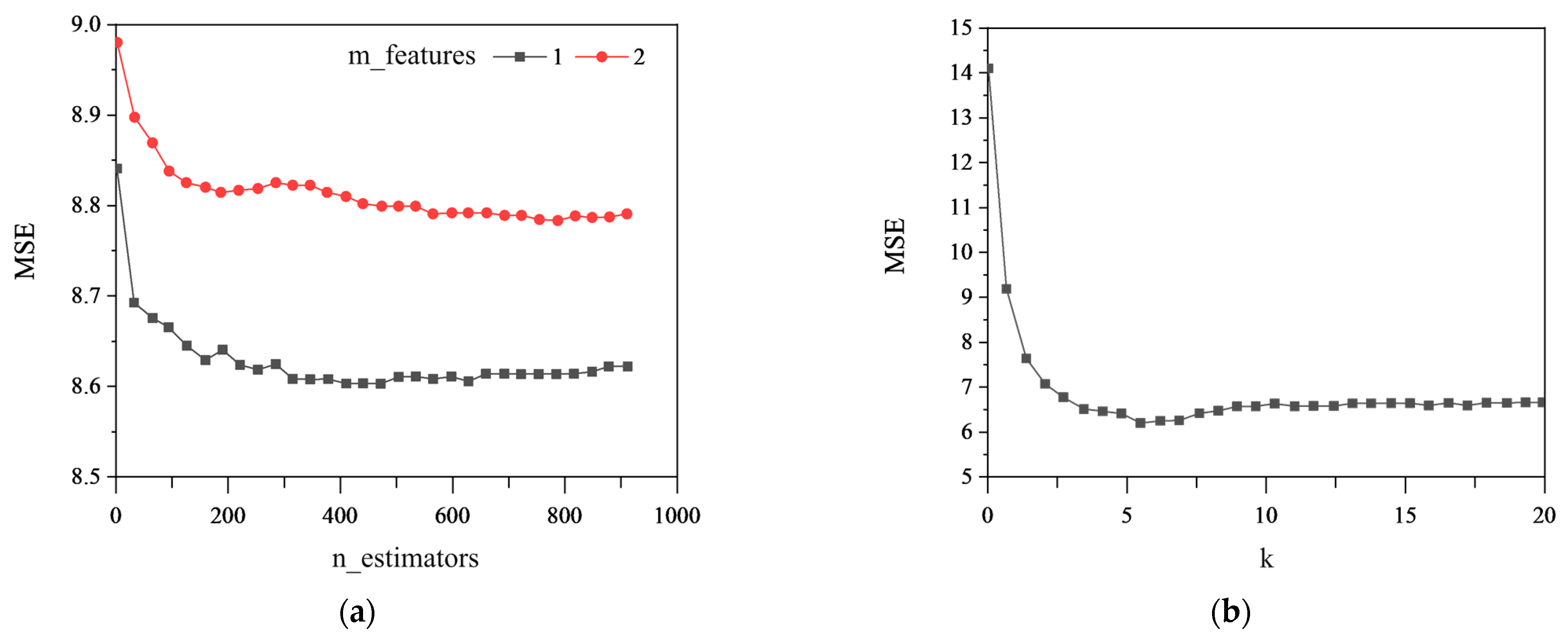
The hyperparameters of the RF and KNN models were selected through 10-fold cross-validation, and the results are presented in Figure 6. Figure 6a shows that the optimal parameters and for the RF model are suitable to select 500 and 1, where is the number of CART decision trees and is the number of selected features. Figure 6b shows that the optimal parameter k for the KNN model is suitable for selecting 7, where k is the number of nearest samples.
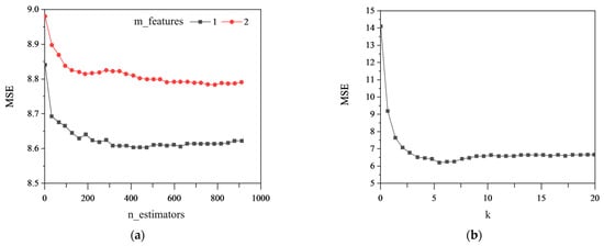
Figure 6.
Hyperparameter selection through 10-fold cross-validation: (a) and of the RF model; (b) k of the KNN model.
(2) Imputation Results Analysis
The combination model based on single-dimensional interpolation and multivariate regression was utilized for imputation, while six baseline models were employed for comparison. The RMSE values calculated using different methods are presented in Table 5. Experimental results show that the multivariate regression model performs better than the single-dimensional interpolation model. And the combination of a single-dimensional interpolation model and a multivariate regression model exhibits improved imputation accuracy. In particular, the combination of single-dimensional interpolation and MLR achieves the highest imputation accuracy, with an RMSE value of only 1.976. This further indicates the significance of considering both the continuity in the time dimension and the correlation between variables when dealing with short-term missing variables.

Table 5.
RMSE of missing data imputation results for continuous missing variables.
4.4.3. Continuous Missing Samples Imputation
In order to evaluate the imputation accuracy of short-term and long-term missing samples, the missing data segments and were imputed based on LSTM model after completing the imputation of all transient isolated missing values and continuous missing variables in data segments , and . The detailed imputation process for continuous missing sample is shown in Section 3.2.4.
(1) Hyperparameters Selection
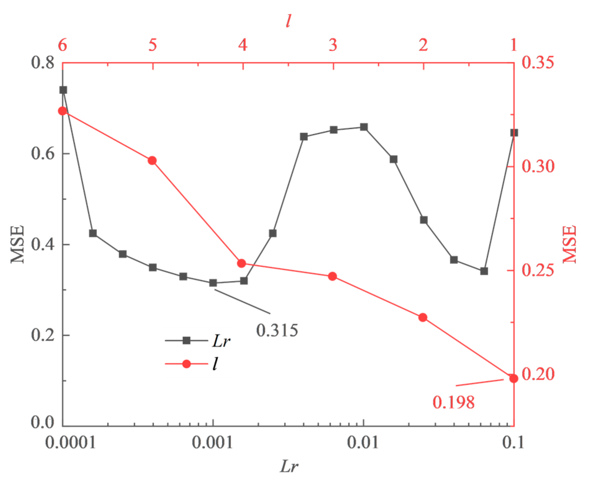
The parameters and have a significant impact on the performance of LSTM, where represents the learning rate and represents the time steps. They were optimized separately, considering their minimal mutual influence. Initially, the LSTM network was initialized with the following parameters: the number of neurons was set to 120, the number of iterations was set to 400, the Adam optimization algorithm was used as the Optimizer, a gradient threshold of 1 was set to prevent gradient explosions, and the dropout rate was set to 0.
The parameters and were selected through 10-fold cross-validation. For , the early stopping technique was applied to prevent overfitting. The frequency of verification was set to 20, and the tolerance of verification was set to 4. While for , the dropout rate was set to 0.2 as a replacement for the early stopping technique to prevent overfitting. The results obtained for parameters and through 10-fold cross-validation are shown in Figure 7.
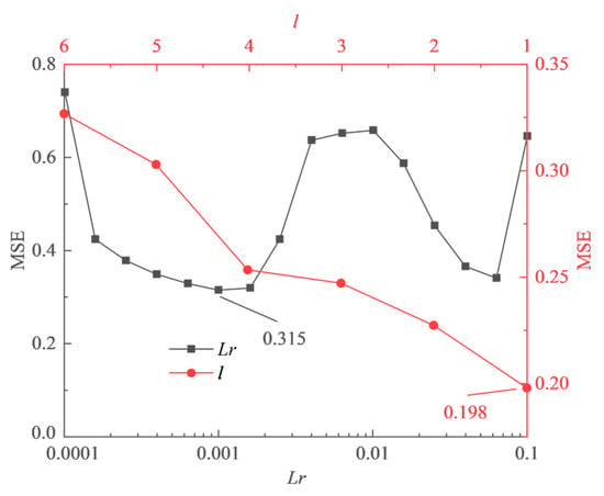
Figure 7.
Hyperparameters selection for LSTM model through 10-fold cross-validation.
As is increased from 0.0001 to 0.1, the MSE curve initially exhibits a rise followed by a decline. However, when exceeds 0.1, training begins to fail. Therefore, is set to 0.001. The MSE curve for shows an almost linearly increasing trend, which indicates that the imputation accuracy will decrease as the historical input data increases. Therefore, is set to 1. In addition, when using the lost layer instead of the early stopping technique to prevent overfitting, the MSE value decreases from 0.315 to 0.198. This indicates that the lost layer is more effective in preventing overfitting than the early stopping technique.
(2) Imputation Results Analysis
The ARIMA (Autoregressive Integrated Moving Average) [43,44] and ELM [36,45] were selected as baseline models. ARIMA is a classical time series model that combines autoregressive, differencing, and moving average components to predict missing values through data autocorrelation. ELM is an efficient machine learning model based on a single-layer feedforward neural network that uses multiple features to predict missing values. The number of hidden layer neurons of both the ELM and LSTM models is the same. The RMSE values calculated for different models are shown in Table 6. The results show that the LSTM model exhibits higher imputation accuracy compared to the ARIMA and ELM models. This indicates that the LSTM model is more effective in capturing long-term dependencies in time series data.

Table 6.
RMSE of missing data imputation results for continuous missing samples.
5. Conclusions
In real-world batch process monitoring datasets, missing data usually occurs in different patterns. Failing to identify the type of missing data or applying imputation methods regardless of the missing type may decrease imputation performance. Many imputation methods have been developed to impute the missing data; however, most of them still do not fulfill the need for data quality in datasets with different types of missing data. Therefore, this paper proposes a novel hybrid missing data imputation method to deal with different types of missing data in a real-world batch process monitoring dataset. By classifying missing data into five distinct categories, we combine and improve suitable models to step-by-step impute different categories of missing data based on their unique characteristics. Through experiments taking a real-world injection molding process monitoring dataset as an example, it can be concluded that missing data pattern analysis combined with appropriate models to impute missing data has better imputation accuracy. Therefore, the hybrid method proposed in this paper excels at missing data imputation for complex batch process monitoring datasets. In practical applications, this method can be employed to impute missing data in batch process monitoring datasets, and the design concept of first categorizing and then stepwise imputing based on data features in this method can also be extended to other datasets containing different types of missing data.
In future research, we plan to conduct studies on the following aspects: The 10-fold cross-validation method, employed for hyperparameter selection in LSTM models, still needs some degree of manual tuning; Bayesian Optimization or Successive Halving could be introduced for automated optimization. Although we have designed a missing data classification method, automated techniques for missing data classification need to be further explored. Data noise can potentially impact imputation performance, and methods such as data cleaning or outlier detection to preprocess the data for noise elimination can be explored. Furthermore, referring to the benchmark proposed in reference [19], additional metrics besides RMSE, such as MAE and runtime, can be introduced. A comprehensive evaluation of imputation accuracy and efficiency could be conducted by selecting suitable baseline methods and utilizing multiple batch process monitoring datasets, while considering various factors like the missing block size, the number of sequences, etc. Based on the evaluation results, the proposed hybrid method might be further improved by enhancing existing models or introducing new models.
Author Contributions
Conceptualization, Y.J. and X.D.; methodology, L.G. and Q.G.; validation, L.G., Q.G. and X.D.; formal analysis, D.H.; writing—original draft preparation, Q.G.; writing—review and editing, Q.G. and X.D.; supervision, D.H., Y.J. and X.D. All authors have read and agreed to the published version of the manuscript.
Funding
This work was supported in part by the National Key R&D Program of China under Grant No. 2020YFB1707900 and 2020YFB1711800; the National Natural Science Foundation of China under Grant No. 62262074, 62172061 and U2268204; the Science and Technology Project of Sichuan Province under Grant No. 2022YFG0159, 2022YFG0155, 2022YFG0157.
Institutional Review Board Statement
Not applicable.
Informed Consent Statement
Not applicable.
Data Availability Statement
Not applicable.
Conflicts of Interest
The authors declare no conflict of interest.
Abbreviations
| LSTM | Long Short-Term Memory |
| LR | Linear Regression |
| MLR | Multivariate Linear Regression |
| SVD | Singular Value Decomposition |
| PCA | Principal Component Analysis |
| MF | Matrix Factorization |
| CD | Centroid Decomposition |
| EM | Expectation Maximization |
| KNN | K Nearest Neighbor |
| RF | Random Forest |
| ELM | Extreme Learning Machine |
| RNNs | Recurrent Neural Networks |
| VMP | Variable Missing Proportion |
| SMP | Sample Missing Proportion |
| CART | Classification and Regression Tree |
| RMSE | Root Mean Square Error |
| MSE | Mean Square Error |
| ARIMA | Autoregressive Integrated Moving Average |
References
- Yao, Y.; Dai, Y.; Luo, W. Early fault diagnosis method for batch process based on local time window standardization and trend analysis. Sensors 2021, 21, 8075. [Google Scholar] [CrossRef] [PubMed]
- Ge, Z.; Gao, F.; Song, Z. Batch process monitoring based on support vector data description method. J. Process Control 2011, 21, 949–959. [Google Scholar] [CrossRef]
- Zhao, L.; Yang, J. Batch process monitoring based on quality-related time-batch 2D evolution information. Sensors 2022, 22, 2235. [Google Scholar] [CrossRef] [PubMed]
- Zhao, Z.; Huang, B.; Liu, F. Bayesian method for state estimation of batch process with missing data. Comput. Chem. Eng. 2013, 53, 14–24. [Google Scholar] [CrossRef]
- Donders, A.R.; van der Heijden, G.J.; Stijnen, T.; Moons, K.G. Review: A gentle introduction to imputation of missing values. J. Clin. Epidemiol. 2007, 59, 1087–1091. [Google Scholar] [CrossRef]
- Zhang, Z. Missing values in big data research: Some basic skills. Ann. Transl. Med. 2015, 3, 323. [Google Scholar] [PubMed]
- Aittokallio, T. Dealing with missing values in large-scale studies: Microarray data imputation and beyond. Brief. Bioinform. 2010, 11, 253–264. [Google Scholar] [CrossRef] [PubMed]
- Nomikos, P.; MacGregor, J.F. Multivariate SPC charts for monitoring batch processes. Technometrics 1995, 37, 41–59. [Google Scholar] [CrossRef]
- Stordrange, L.; Rajalahti, T.; Libnau, F.O. Multiway methods to explore and model NIR data from a batch process. Chemom. Intell. Lab. Syst. 2004, 70, 137–145. [Google Scholar] [CrossRef]
- Meng, X.; Morris, A.; Martin, E. On-line monitoring of batch processes using a PARAFAC representation. J. Chemom. 2003, 17, 65–81. [Google Scholar] [CrossRef]
- Shi, W.; Zhu, Y.; Huang, T.; Sheng, G.; Lian, Y.; Wang, G.; Chen, Y. An integrated data preprocessing framework based on apache spark for fault diagnosis of power grid equipment. J. Signal Process. Syst. 2017, 86, 221–236. [Google Scholar] [CrossRef]
- Emmanuel, T.; Maupong, T.; Mpoeleng, D.; Semong, T.; Mphago, B.; Tabona, O. A survey on missing data in machine learning. J. Big Data 2021, 8, 1–37. [Google Scholar] [CrossRef]
- García-Laencina, P.J.; Sancho-Gómez, J.-L.; Figueiras-Vidal, A.R. Pattern classification with missing data: A review. Neural Comput. Appl. 2010, 19, 263–282. [Google Scholar] [CrossRef]
- Lin, W.-C.; Tsai, C.-F. Missing value imputation: A review and analysis of the literature (2006–2017). Artif. Intell. Rev. 2020, 53, 1487–1509. [Google Scholar] [CrossRef]
- Farhangfar, A.; Kurgan, L.A.; Pedrycz, W. A novel framework for imputation of missing values in databases. IEEE Trans. Syst. Man Cybern. Part A Syst. Hum. 2007, 37, 692–709. [Google Scholar] [CrossRef]
- Andridge, R.R.; Little, R.J. A review of hot deck imputation for survey non-response. Int. Stat. Rev. 2010, 78, 40–64. [Google Scholar] [CrossRef] [PubMed]
- Langkamp, D.L.; Lehman, A.; Lemeshow, S. Techniques for handling missing data in secondary analyses of large surveys. Acad. Pediatr. 2010, 10, 205–210. [Google Scholar] [CrossRef]
- Yu, L.; Liu, L.; Peace, K.E. Regression multiple imputation for missing data analysis. Stat. Methods Med. Res. 2020, 29, 2647–2664. [Google Scholar] [CrossRef] [PubMed]
- Khayati, M.; Lerner, A.; Tymchenko, Z.; Cudre-Mauroux, P. Mind the gap: An experimental evaluation of imputation of missing values techniques in time series. Proc. Vldb. Endow. 2020, 13, 768–782. [Google Scholar] [CrossRef]
- Papadimitriou, S.; Sun, J.; Faloutos, C.; Yu, P.S. Dimensionality reduction and filtering on time series sensor streams. In Managing and Mining Sensor Data; Aggarwal, C.C., Ed.; Springer: Boston, MA, USA, 2013; pp. 103–141. [Google Scholar]
- Shu, X.B.; Porikli, F.; Ahuja, N. Robust orthonormal subspace learning: Efficient recovery of corrupted low-rank matrices. In Proceedings of the IEEE Conference on Computer Vision and Pattern Recognition, Columbus, OH, USA, 23–28 June 2014. [Google Scholar]
- Mazumder, R.; Hastie, T.; Tibshirani, R. Spectral regularization algorithms for learning large incomplete matrices. J. Mach. Learn. Res. 2010, 11, 2287–2322. [Google Scholar]
- Yu, H.-F.; Rao, N.; Dhillon, I.S. Temporal regularized matrix factorization for high-dimensional time series prediction. In Proceedings of the Advances in Neural Information Processing Systems, Barcelona, Spain, 5–10 December 2016. [Google Scholar]
- Khayati, M.; Böhlen, M.H.; Mauroux, P.C. Using lowly correlated time series to recover missing values in time series: A comparison between SVD and CD. In Proceedings of the Advances in Spatial and Temporal Databases: 14th International Symposium, Hong Kong, China, 26–28 August 2015. [Google Scholar]
- Yi, X.; Zheng, Y.; Zhang, J.; Li, T. ST-MVL: Filling missing values in geo-sensory time series data. In Proceedings of the 25th International Joint Conference on Artificial Intelligence, New York, NY, USA, 9–15 July 2016. [Google Scholar]
- Li, L.; McCann, J.; Pollard, N.; Faloutsos, C. DynaMMo: Mining and summarization of coevolving sequences with missing values. In Proceedings of the 15th ACM SIGKDD International Conference on Knowledge Discovery and Data Mining, Paris, France, 28 June–1 July 2009. [Google Scholar]
- Kim, T.; Kim, J.; Yang, W.; Lee, H.; Choo, J. Missing value imputation of time-series air-quality data via deep neural networks. Int. J. Environ. Res. Public Health 2021, 18, 12213. [Google Scholar] [CrossRef] [PubMed]
- Chen, Y.; Gu, C.; Shao, C.; Gu, H.; Zheng, D.; Wu, Z.; Fu, X. An approach using adaptive weighted least squares support vector machines coupled with modified ant lion optimizer for dam deformation prediction. Math. Probl. Eng. 2020, 2020, 9434065. [Google Scholar] [CrossRef]
- Wei, W.; Gu, C.; Fu, X. Processing method of missing data in dam safety monitoring. Math. Probl. Eng. 2021, 2021, 9950874. [Google Scholar] [CrossRef]
- Nadimi-Shahraki, M.H.; Mohammadi, S.; Zamani, H.; Gandomi, M.; Gandomi, A.H. A hybrid imputation method for multi-pattern missing data: A case study on type II diabetes diagnosis. Electronics 2021, 10, 3167. [Google Scholar] [CrossRef]
- Liang, X.; Ge, Z.; Sun, L.; He, M.; Chen, H. LSTM with wavelet transform based data preprocessing for stock price prediction. Math. Probl. Eng. 2019, 2019, 1340174. [Google Scholar] [CrossRef]
- Maillo, J.; Ramírez, S.; Triguero, I.; Herrera, F. kNN-IS: An Iterative Spark-based design of the k-Nearest Neighbors classifier for big data. Knowl.-Based Syst. 2017, 117, 3–15. [Google Scholar] [CrossRef]
- Tang, F.; Ishwaran, H. Random forest missing data algorithms. Stat. Anal. Data Min. ASA Data Sci. J. 2017, 10, 363–377. [Google Scholar] [CrossRef]
- Hong, S.; Lynn, H.S. Accuracy of random-forest-based imputation of missing data in the presence of non-normality, non-linearity, and interaction. BMC Med. Res. Methodol. 2020, 20, 199. [Google Scholar] [CrossRef]
- Raja, P.S.; Thangavel, K. Missing value imputation using unsupervised machine learning techniques. Soft Comput. 2020, 24, 4361–4392. [Google Scholar] [CrossRef]
- Huang, G.-B.; Zhu, Q.-Y.; Siew, C.-K. Extreme learning machine: Theory and applications. Neurocomputing 2006, 70, 489–501. [Google Scholar] [CrossRef]
- Song, W.; Gao, C.; Zhao, Y.; Zhao, Y. A time series data filling method based on LSTM-Taking the stem moisture as an example. Sensors 2020, 20, 5045. [Google Scholar] [CrossRef] [PubMed]
- Yoon, J.; Zame, W.R.; van der Schaar, M. Estimating missing data in temporal data streams using multi-directional recurrent neural networks. IEEE Trans. Biomed. Eng. 2018, 66, 1477–1490. [Google Scholar] [CrossRef] [PubMed]
- Dyer, S.A.; Xin, H. Cubic-spline interpolation: Part 2. IEEE Instrum. Meas. Mag. 2001, 4, 34–36. [Google Scholar] [CrossRef]
- Cover, T.; Hart, P. Nearest neighbor pattern classification. IEEE Trans. Inf. Theory 1967, 13, 21–27. [Google Scholar] [CrossRef]
- Srivastava, N.; Hinton, G.; Krizhevsky, A.; Sutskever, I.; Salakhutdinov, R. Dropout: A simple way to prevent neural networks from overfitting. J. Mach. Learn. Res. 2014, 15, 1929–1958. [Google Scholar]
- The Injection Molding Process Monitoring Dataset. Available online: https://github.com/Chow-kk/DATASET_4th_industrial-bigdata_competion_ (accessed on 1 March 2022).
- Kohn, R.; Ansley, C.F. Estimation, prediction, and interpolation for ARIMA models with missing data. J. Am. Stat. Assoc. 1986, 81, 751–761. [Google Scholar] [CrossRef]
- Sura, T.; Nassir, A.B.K.; Wassan, T. Mousa Estimation the missing data of meteorological variables in different Iraqi cities by using ARIMA model. Iraqi J. Sci. 2018, 59, 792–801. [Google Scholar]
- Sovilj, D.; Eirola, E.; Miche, Y.; Björk, K.-M.; Nian, R.; Akusok, A.; Lendasse, A. Extreme learning machine for missing data using multiple imputations. Neurocomputing 2016, 174, 220–231. [Google Scholar] [CrossRef]
Disclaimer/Publisher’s Note: The statements, opinions and data contained in all publications are solely those of the individual author(s) and contributor(s) and not of MDPI and/or the editor(s). MDPI and/or the editor(s) disclaim responsibility for any injury to people or property resulting from any ideas, methods, instructions or products referred to in the content. |
© 2023 by the authors. Licensee MDPI, Basel, Switzerland. This article is an open access article distributed under the terms and conditions of the Creative Commons Attribution (CC BY) license (https://creativecommons.org/licenses/by/4.0/).


