In this section, the M-CVAE model is applied to two real industrial cases for soft sensors. To evaluate the performance of the proposed M-CVAE, three indexes, the mean absolute error (MAE), the root mean square error (RMSE), and the coefficient of determination index R2, are calculated comparing the results with other regression models.
3.3.1. Debutanizer Column
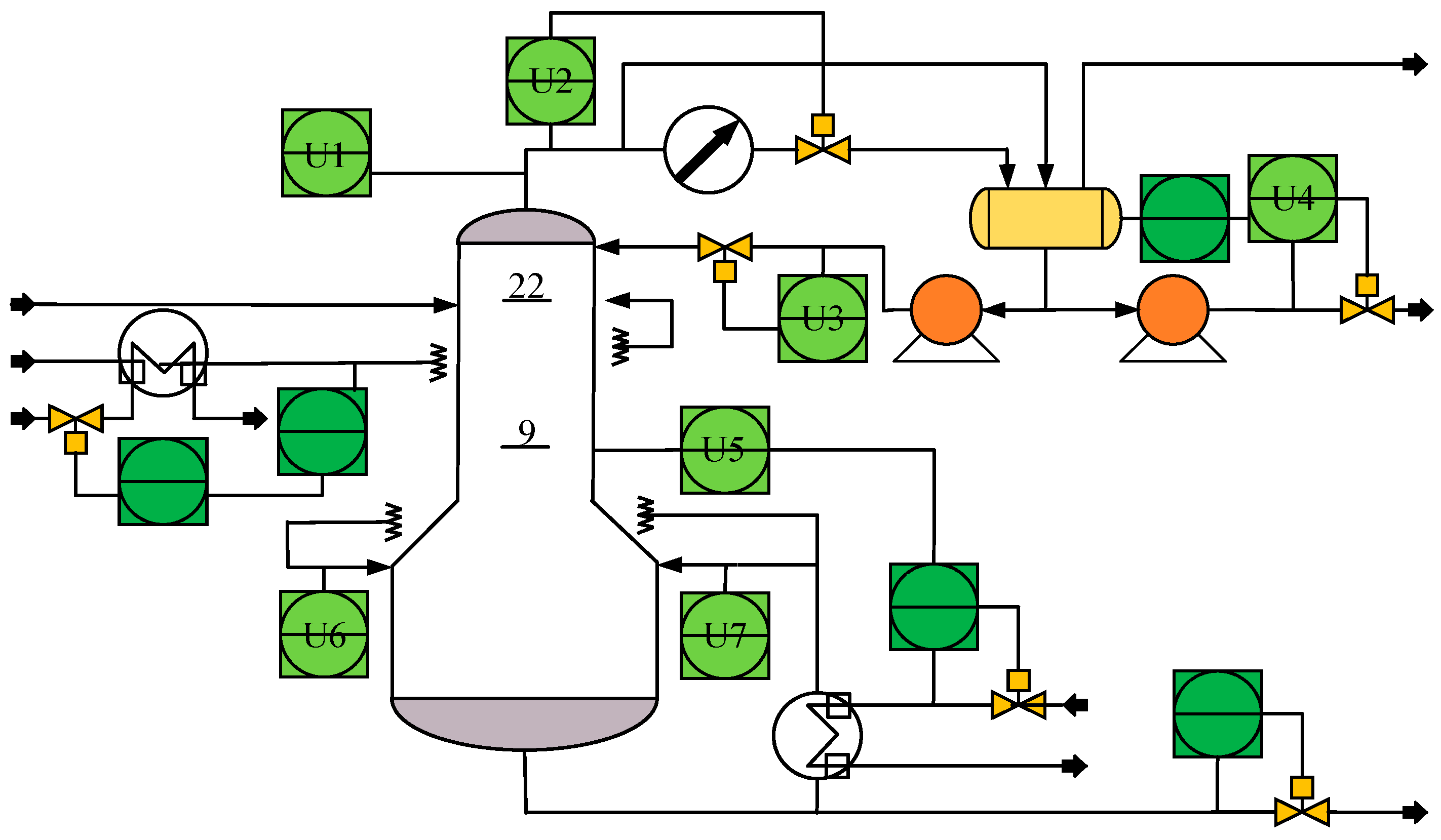
The debutanizer column is an important part of the refinery process in petroleum production processes, which can separate propane and butane from the naphtha stream [
33]. The process flowchart is shown in
Figure 4. Due to the butane content at the bottom of the debutanizer column being very low, the measurement of butane concentration is difficult and there is usually a great delay. Therefore, it is valuable to introduce the soft senor for butane concentration.
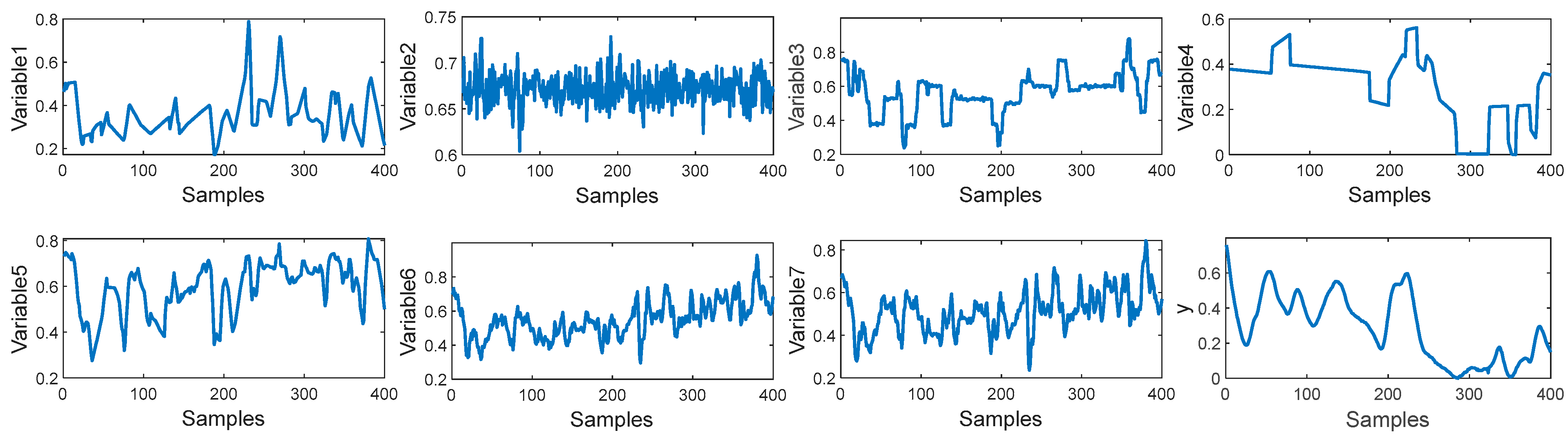
In this paper, a total of 2394 samples have been collected from the debutanizer column. The first 1900 samples are used for the training set and the last 400 samples are used for the test set. Seven process variables are selected as the input of the M-CVAE model to predict the butane concentration and a detailed description of the seven process variables and the output of the predicted variable is shown in
Table 1. The trend of input variables and output variables is shown in
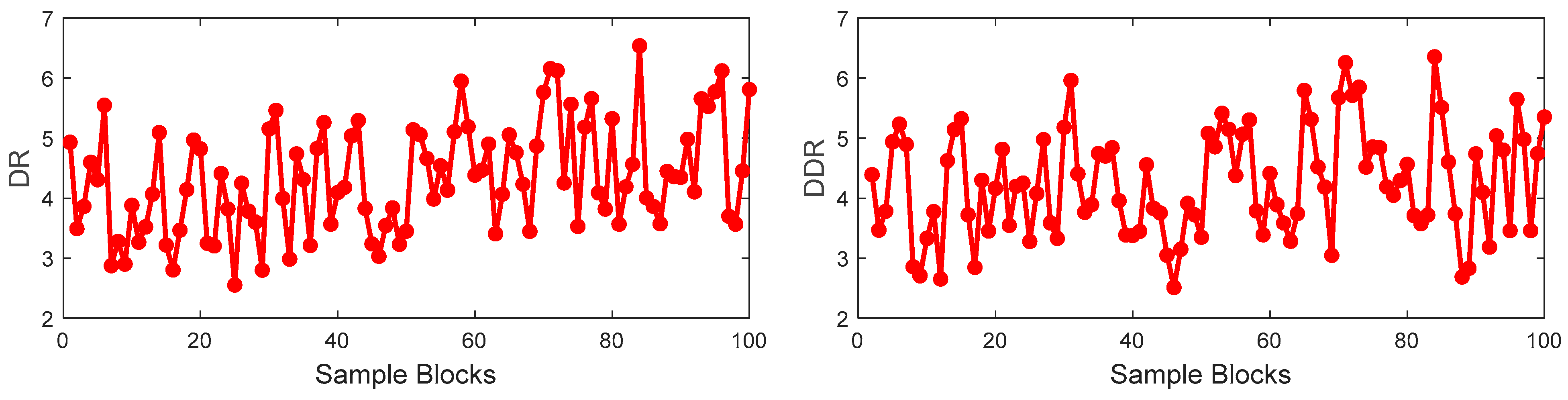
Figure 5. It can be seen that the input of these variables has obvious fluctuations, which indicates that there is significant nonlinearity in such a process. In order to demonstrate the nonlinearity between the input variables and output variables, the degree of repeatability (DR) and the differential degree of repeatability (DDR) are introduced [
34]. The DR and DDR can reflect the similarity and difference of the correlation of the sample blocks.
Firstly, the training set is divided into 100 blocks with 19 samples in each block. The DR of each block and the DDR of two adjacent blocks are calculated as shown in
Figure 6. In
Figure 6, the values of the DR and DDR have random change among the sample blocks, which indicates that the correlation between input and output is not consistent throughout the whole process. It is illustrated that the nonlinearity between the process variables and output variable is obvious.
Based on the training data set, the M-CVAE model is built. For comparison, the other soft sensor models including PLS, SVR, DVAE, and Supervised NDS models are also built. Here, DVAE is supervised VAE proposed in the paper [
30]. Supervised NDS is a supervised nonlinear dynamic model composed of VAE, a neural network and dynamic system, which is proposed in the paper [
27].
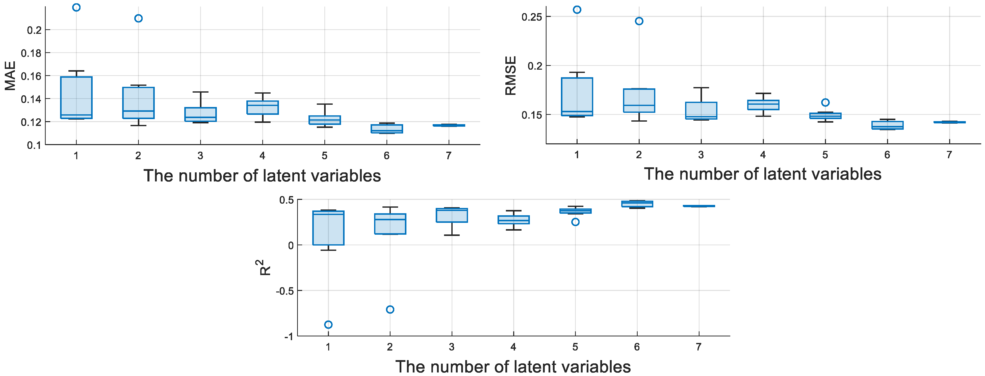
The encoder of M-CVAE consists of three convolutional layers and a fully connected layer, and the decoder consists of three deconvolution layers and a fully connected layer. The number of convolution kernels is 32, the size of the convolution kernel is 3 × 3, and the activation function is the Relu function. The number of latent variables is a key parameter, which affects the performance of the model to a certain extent. Therefore, the average evaluation indices of MAE, RMSE, and R
2 for the M-CVAE model, which are based on the seven test experiments, are shown in
Figure 7. It can show the fluctuation degree of MAE, RMSE, and R
2 with different numbers of latent variables. That is to say, the smaller the rectangular area, the more stable the performance of the model.
Therefore, it can be seen that the M-CVAE model has the most stable performance when the number of latent variables is 7. While the number of latent variables is 6, more optimal values of MAE, RMSE, and R
2 can be obtained. Also, the stable performance is quite excellent. Furthermore, the optimal values of MAE, RMSE, and R
2 corresponding to different numbers of latent variables are given in
Table 2. From
Table 2, it can be seen that the optimal values of MAE, RMSE, and R
2 are obtained when the number of latent variables is 6. Finally, the number of latent variables is determined as 6 for the M-CVAE model from a comprehensive point. Meanwhile, the optimal number of latent variables is also selected for other regression models.
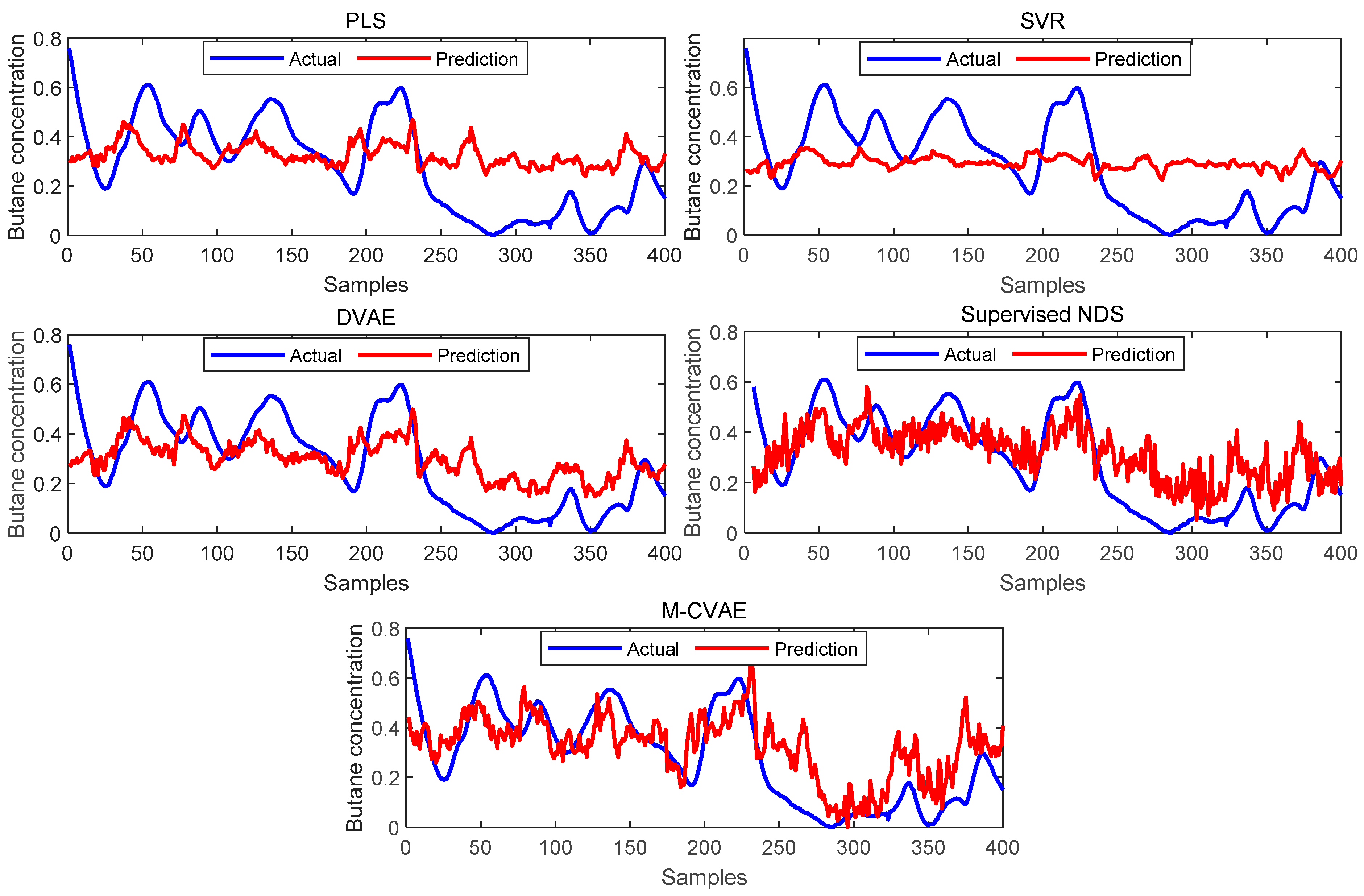
The prediction results of PLS, SVR, DVAE, Supervised NDS, and the proposed M-CVAE method are shown in
Figure 8. From
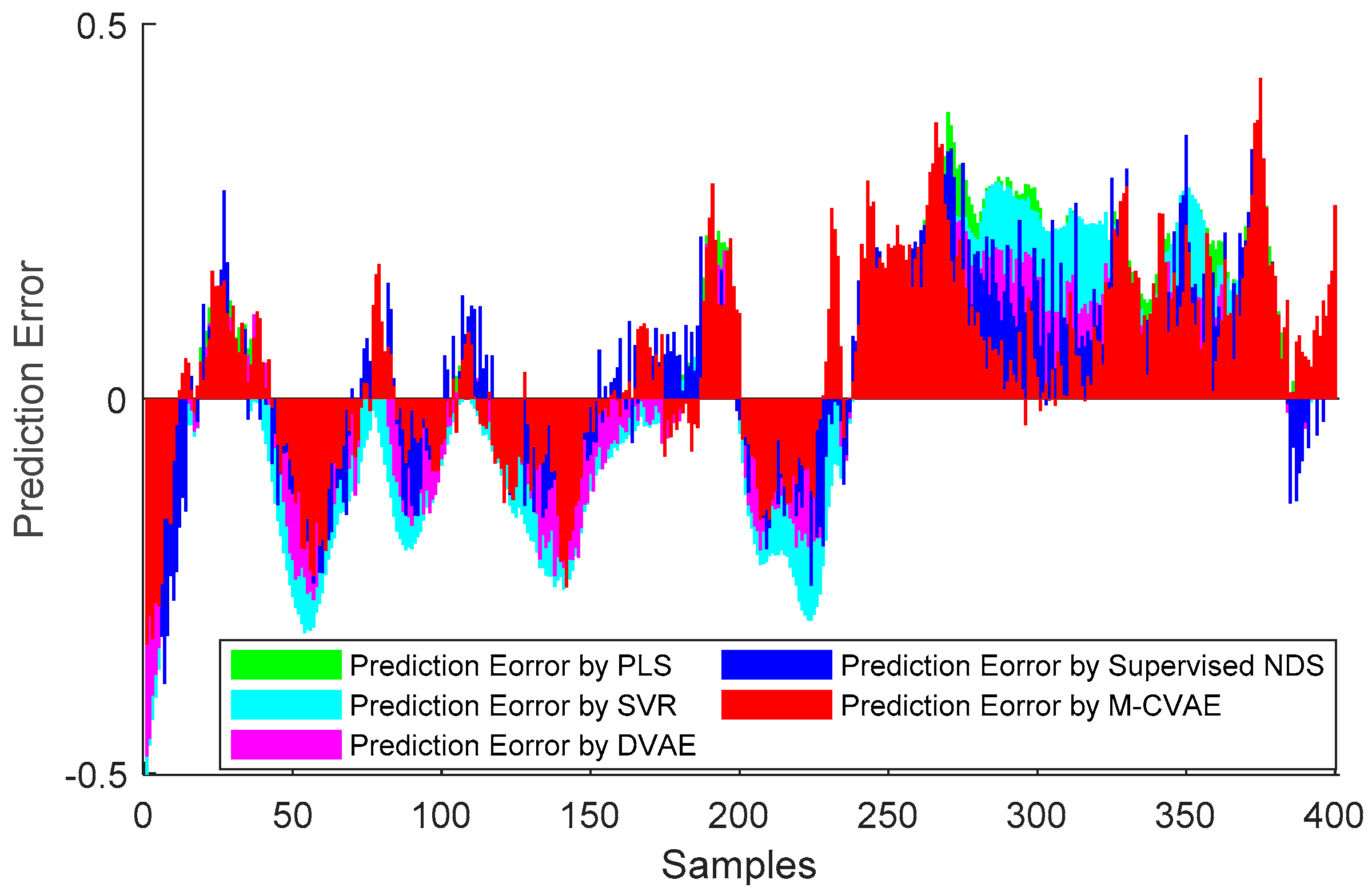
Figure 8, it is not difficult to see that the predicted butane concentration based on the M-CVAE method is closest to the actual value in most of the process. It also can be seen that neither PLS nor SVR can fit the actual values well. The reason is that traditional machine learning methods are based on shallow learning, which cannot deeply mine complex nonlinearity in data. The M-CVAE has a deep generative model composed of multi-layer networks, which can well mine the nonlinear characteristics of data. With DVAE and Supervised NDS as deep learning methods, there is a better fluctuation trend of tracking the actual value. However, the fitting degree of these two methods has declined with obvious fluctuation. This is because the data generation based on both the DVAE and Supervised NDS model is similar to the traditional VAE model. While data generation is based on VAE, no constraints are introduced to the model, and as a result, the resampling can be carried out in the whole latent space. This can cause instability and uncontrollability issues in data generation. It is because as the encoding area expands, the resampling range also expands due to the noise introduced in the VAE framework. This may lead to strengthen the randomness and uncertainty of resampling, increase the sampling probability far from the original data code area, and decrease the probability of the original code area. It means that the constraint of the original data to resampling is reduced, which to some extent causes the uncontrollability and randomness of data generation. As a result, the generated data (estimated original data) output from the decoder are not as close as possible to the original data. Compared with DVAE and Supervised NDS, the proposed M-CVAE method has better traceability even at obvious fluctuation, such as samples 80th–130th, 180th–230th, and 255th–350th. The reason why M-CVAE can display the superior performance of prediction is that both process variables and butane concentration can be considered in the M-CVAE model instead of just considering process variables in DVAE and Supervised NDS. In this way, nonlinearity between process variables and butane concentration can be well extracted so that it is quite helpful for the regression model to improve the performance of prediction. It is more important that M-CVAE can control the predicted value close to the actual value by a condition instead of outputting the predicted value only according to a probability distribution, which can improve the controllability and stability of the model. In addition, labels or conditions input to the encoder and decoder are changeable with the input data. That is to say, the input data are always input to the encoder and decoder together with the matching label. Therefore, the dynamic label always can specify generated data as close as possible to the current input sample. This ensures the generalization ability and robustness of the model. Furthermore, the error prediction of all the methods is shown in
Figure 9 for comparison. From
Figure 9, it can be seen that the proposed M-CVAE method has the smallest error in most of the process. The detailed MAE, RMSE, and R
2 are given in
Table 3. From
Table 3, we can see that M-CVAE has the lowest MAE and RMSE and the highest R
2 among all the methods. Therefore, it can be demonstrated that the soft sensor based on M-CVAE has optimal performance.
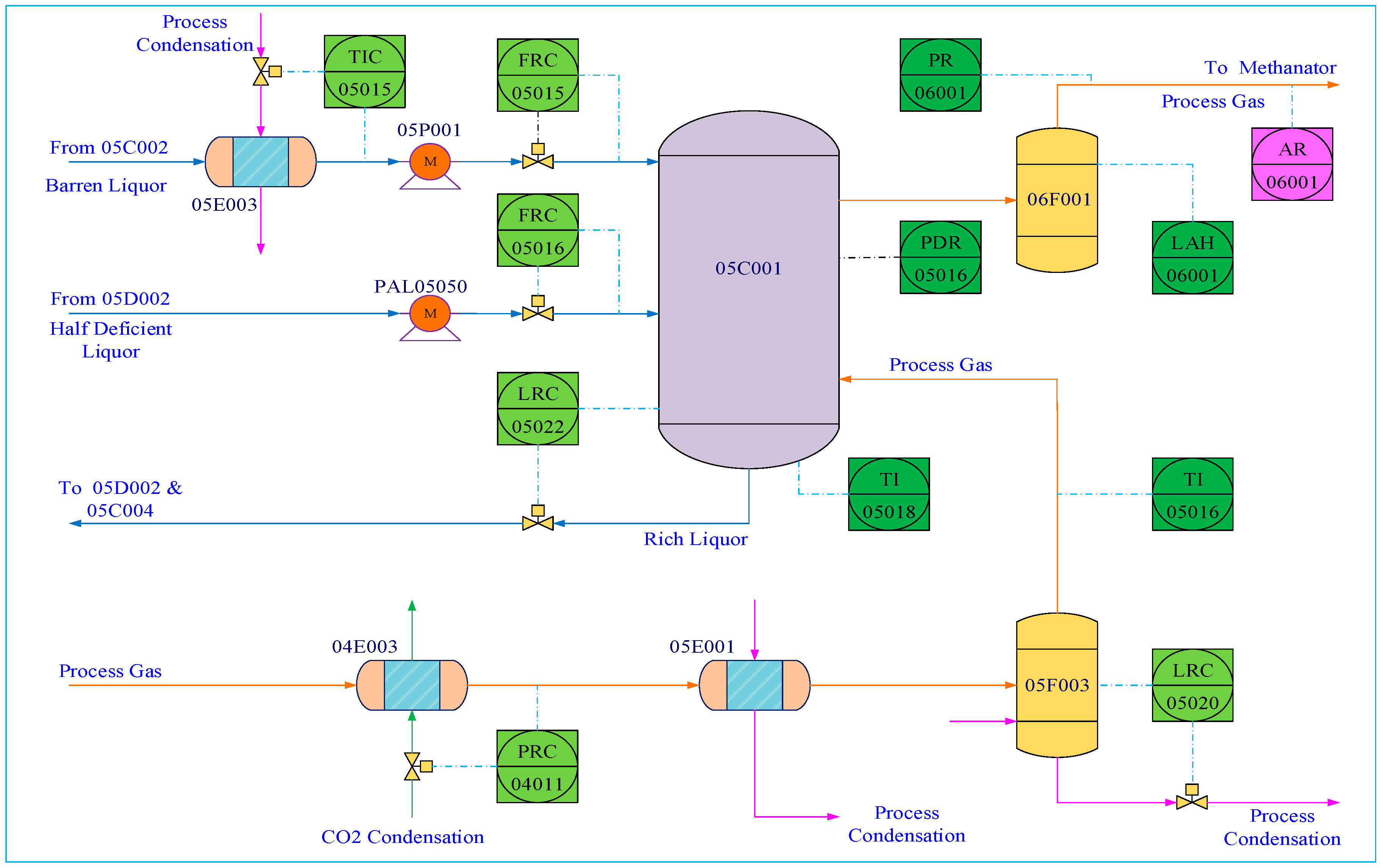
3.3.2. CO2 Absorption Column
The Ammonia synthesis process is a common industrial process for producing NH
3 used as the basic material for Urea synthesis. In this process, NH
3 is produced as well as CO
2 so CO
2 should be further separated. Therefore, the CO
2 absorption column is an important unit in Ammonia synthesis for CO
2 separation, and CO
2 content is a key variable for quality control. The flowchart of the CO
2 absorption column is given in
Figure 10.
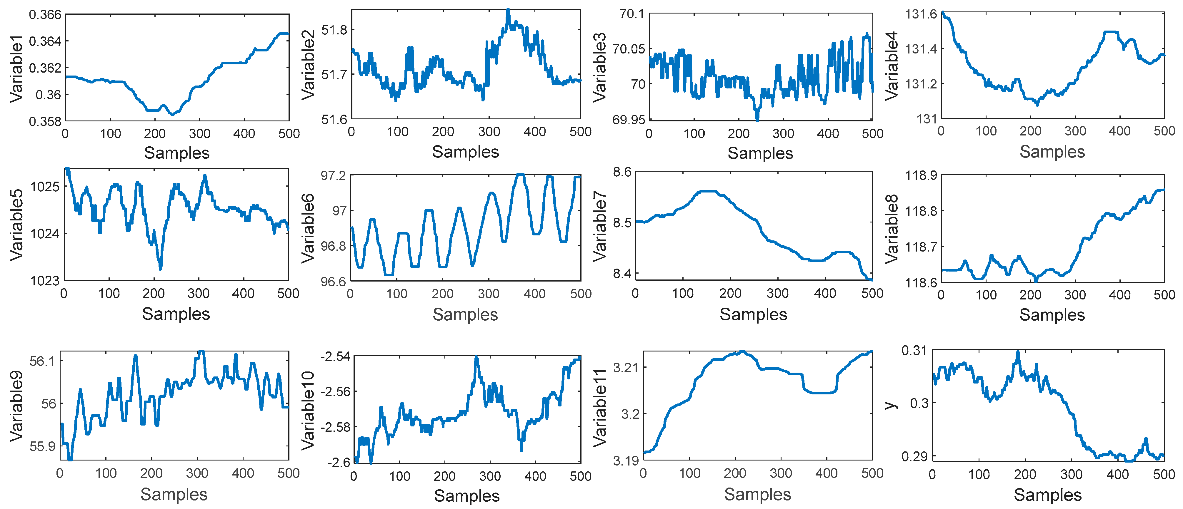
In this paper, 11 process variables are selected for CO
2 content prediction, which are listed in
Table 4. A total of 30,000 samples are collected, in which the first 2000 samples are used as the training data set and the last 500 samples are used as the test data set. The trend of input variables and output variables is shown in
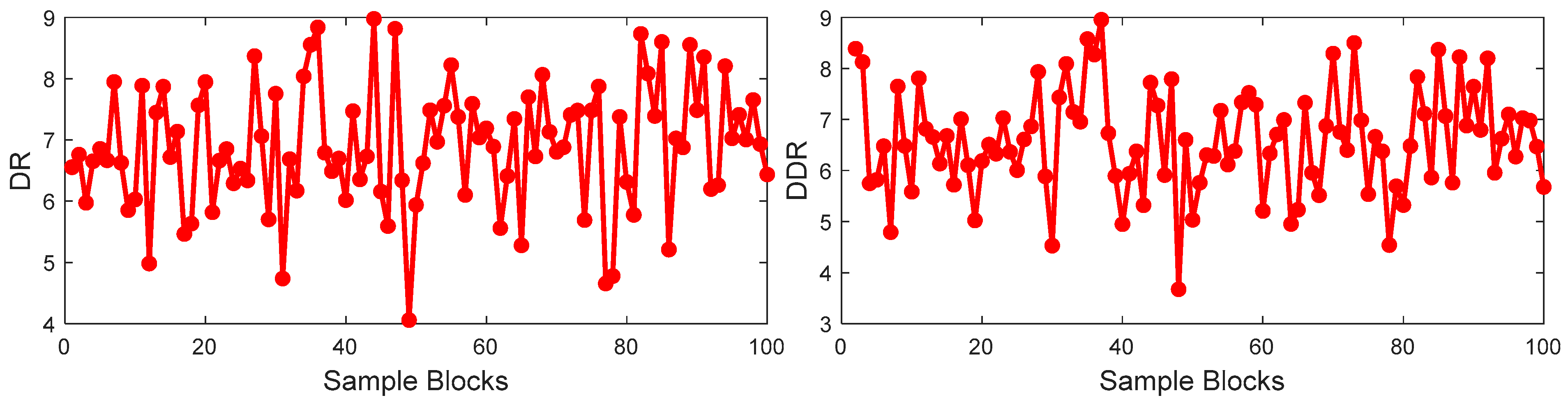
Figure 11. It can be seen that the input variables and output variable have obvious fluctuation. It can be inferred that this process has a strong nonlinearity. To illustrate the nonlinearity between the input and output, the training set is divided into 100 blocks with 40 samples in each block. The DR of each block and the DDR of two adjacent blocks are shown in
Figure 12. In
Figure 12, the values of DR and DDR have a significant fluctuation, which illustrates that the nonlinearity between the process variables and output variable is obvious.
Based on the training data set, the model is built. The soft sensor model based on the proposed M-CVAE, PLS, SVR, DVAE, and Supervised NDS model is built. The encoder of M-CVAE consists of five convolutional layers and a fully connected layer, and the decoder consists of five deconvolution layers and a fully connected layer. The number of convolution kernels is 32, the size of the convolution kernel is 3 × 3, and the activation function is the Relu function. Similarly, the number of latent variables for the M-CVAE is determined based on the average evaluation indices of MAE, RMSE, and R
2. The average evaluation index based on 11 test experiments is listed in
Table 5. From
Table 5, it can be seen that the optimal values of MAE, RMSE, and R
2 are obtained when the number of latent variables is 11.
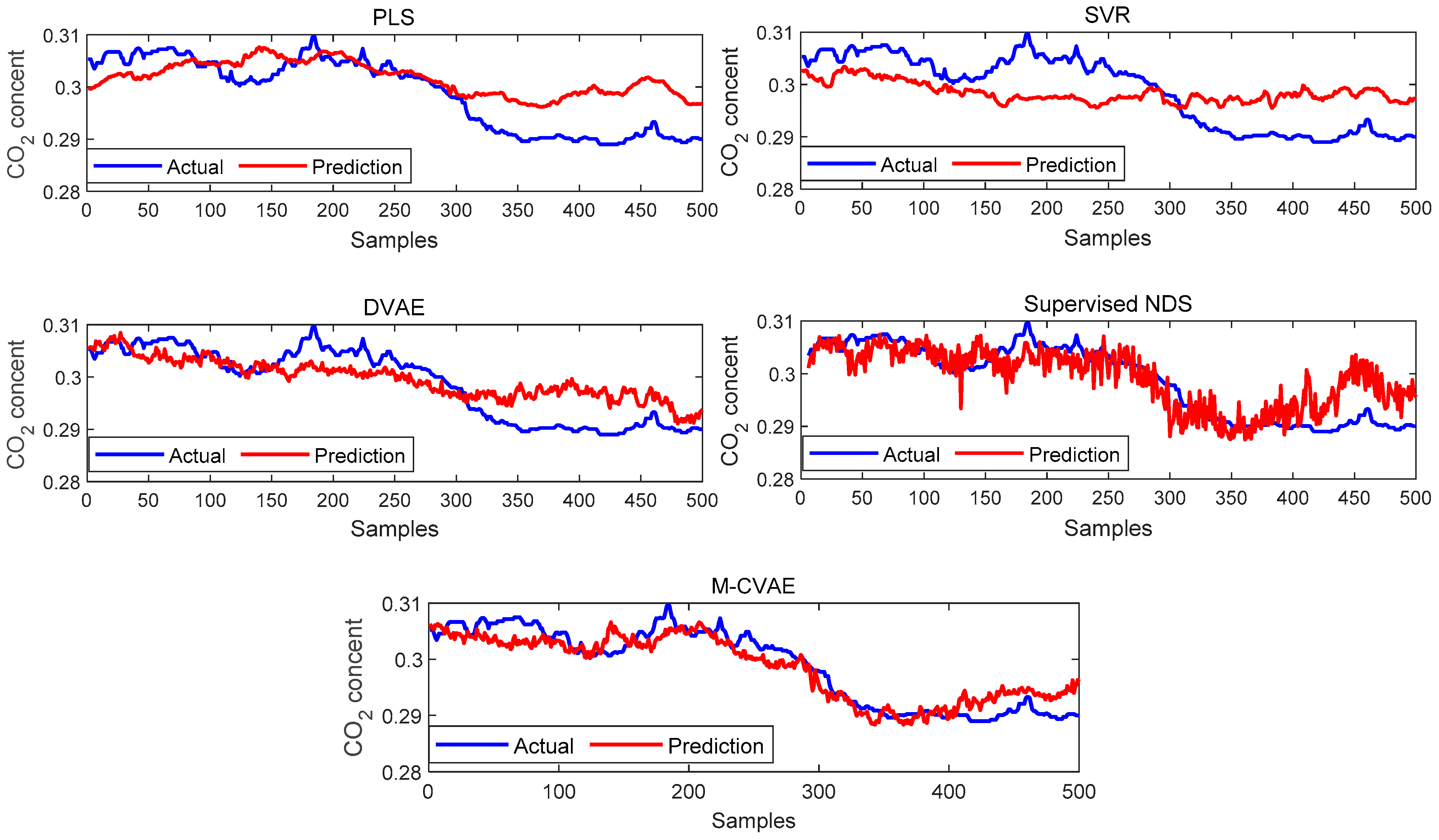
The prediction results of PLS, SVR, DVAE, Supervised NDS, and M-CVAE are shown in
Figure 13. From
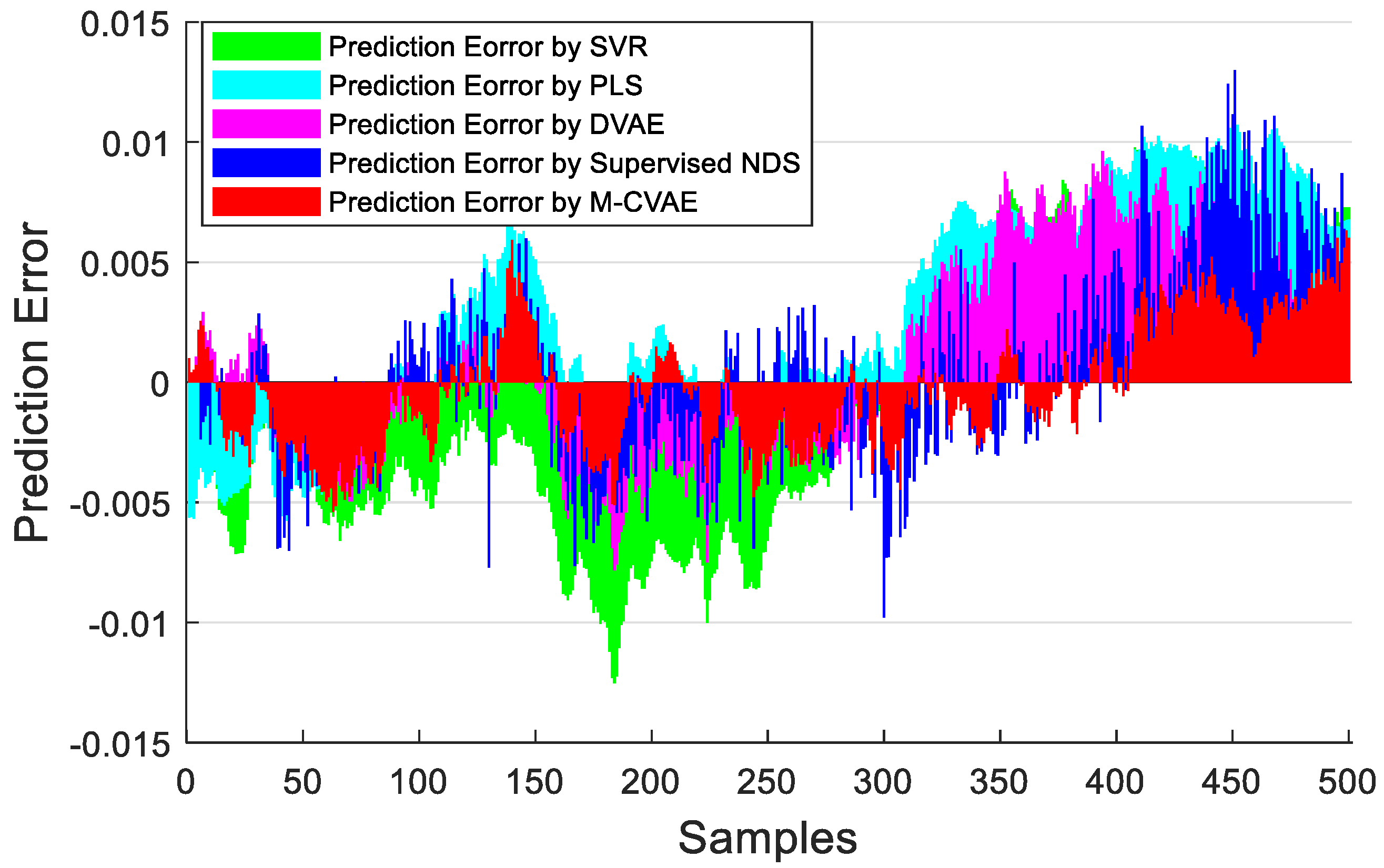
Figure 13, it can be seen that the prediction results based on PLS and SVR show a poor tracking performance. This is because the shallow learning method cannot extract the underlying complex nonlinearity of the data set enough. While the prediction results based on the DVAE and Supervised NDS have a significant improvement in tracking ability in the first 300 samples, it is due to the deep extraction on nonlinearity. However, it can be found that DVAE and Supervised NDS also have a weak prediction performance after about the 300th sample. Instead, the proposed M-CVAE model has an outstanding tracking capacity throughout the process, especially in the last 200 samples with a big change. The reason is that the DCVAE and Supervised NDS model cannot solve the instability and uncontrollability problems in VAE model data generation. This is because, with the expansion of the coding area, the randomness and uncertainty of the sampling will also increase, increasing the uncontrollability and randomness of the generated data. As a result, the similarity between the generated data output by the decoder and the original data is reduced. On the contrary, the M-CVAE model constrains the sampling range of the specified label area by adding the label of the original data as a condition to the model. In this way, the generated data can be closer to the original data, and the generalization ability and robustness of the model can be ensured. Because the labels’ input to the encoder and decoder will change with the input data, the input data is always input to the encoder and decoder together with the matched labels. Therefore, the label always specifies that the generated data are as close as possible to the current input sample. In this way, the M-CVAE shows superior fitting performance, even in a big fluctuation. The prediction error is further shown in
Figure 14. The detailed information of MAE, RMSE, and R
2 are given in
Table 6. From
Figure 14 and
Table 6, it can be seen that the performance of prediction of the proposed M-CVAE model is superior to other methods.


