Abstract
To reduce the influence of gain-phase errors and improve the performance of direction-of-arrival (DOA) estimation, a robust sparse Bayesian two-dimensional (2D) DOA estimation method with gain-phase errors is proposed for L-shaped sensor arrays. The proposed method introduces an auxiliary angle to transform the 2D DOA estimation problem into two 1D angle estimation problems. A sparse representation model with gain-phase errors is constructed using the diagonal element vector of the cross-correlation covariance matrix of two submatrices of the L-shaped sensor array. The expectation maximization algorithm derives unknown parameter expression, which is used for iterative operations to obtain off-grid and signal precision. Using these parameters, a new spatial spectral function is constructed to estimate the auxiliary angle. The obtained auxiliary angle is substituted into a sparse representation model with gain and phase errors, and then the sparse Bayesian learning method is used to estimate the elevation angle of the incident signal. Finally, according to the relationship of the three angles, the azimuth angle can be estimated. The simulation results show that the proposed method can effectively realize the automatic matching of the azimuth and elevation angles of the incident signal, and improves the accuracy of DOA estimation and angular resolution.
1. Introduction
The estimation of the direction-of-arrival of sensor arrays is an important research direction in the fields of radar, sonar and mobile communications, which has attracted the interest of many scholars [1,2,3]. At present, the research on uniform linear arrays (ULAs) is relatively mature, and many high-resolution DOA estimation methods have been proposed to improve the accuracy and resolution, such as the subspace method [4,5], maximum likelihood methods [6,7] and compressed sensing methods. Compared with the first two types of methods, the DOA estimation method based on compressed sensing can effectively estimate the incident angle in the case of a few snapshots and low signal-to-noise ratio (SNR). The reconstruction methods of compressed sensing technology are mainly divided into three categories: convex optimization methods [8,9], greedy iteration methods [10,11] and sparse Bayesian learning (SBL) methods.
Among these methods, by exploring the spatial sparsity of incident signals, sparse Bayesian learning methods have better adaptive performance than the other traditional methods under the conditions of a limited number of snapshots, low SNR and spatially adjacent signals. The SBL method [12], compared with convex optimization methods, not only has the same global convergence, but also has relatively higher computational efficiency. Although the SBL estimation method improves the resolution, its estimation performance is limited by the degree of spatial dispersion. Increasing the estimation accuracy by adding a preset grid will bring a huge computational burden; however, the estimation accuracy will be reduced without increasing the preset grid, that is, there is a mesh mismatch problem. Therefore, Yang et al. [13] considered introducing an off-grid model and proposed an off-grid Sparse Bayesian Inference (OGSBI) method, which further reduced the influence of grid mismatch and improved the DOA estimation accuracy. Dai et al. [14] proposed a root-off grid sparse Bayesian learning (RootSBL) DOA estimation method, which improves the operation efficiency by ensuring high direction estimation accuracy. However, because the off-grid models in the above two methods use first-order Taylor expansion, their estimation performance under a coarse grid is not satisfactory. To solve this problem, the authors of [15] introduced second-order Taylor approximation into off-grid DOA estimation. Although the higher-order Taylor approximation reduces the approximate error and improves the accuracy of DOA estimation, it also increases the computational complexity. In order to reduce the amount of computation, Refs. [16,17] introduced different forms of real-value transformation, using compressed sensing technology to transform the data in the complex number field into the real number field and reduce the operation time of each iteration. Then, for different application backgrounds such as color noise and broadband signals, many researchers used the DOA estimation methods based on variational sparse Bayes [18,19,20], and the DOA estimation performances of such methods were further improved using SBL. Nevertheless, the above methods based on sparse Bayesian learning are all based on ULAs, which can only provide one-dimensional angle information. In practical applications, it is more useful to obtain the 2D direction of the source, that is, the azimuth angle and the elevation angle. In recent years, the research on 2D DOA estimation has gradually increased, and scholars have proposed many array geometries for 2D estimation, such as circular arrays, rectangular arrays and cross arrays. Compared with these 2D arrays, L-shaped arrays are simpler in structure, easier to implement, and have better estimation performance, which has attracted much attention [21].
Although the above types of estimation methods have good DOA estimation performances, they depend on the ideal array manifold, while in practical application scenarios, array manifolds are often affected by unknown gain-phase errors. Without array manifold calibration, the performance of DOA estimation may be greatly degraded [22]. Therefore, the study of DOA estimation methods with array gain-phase errors has theoretical significance and practical value. Of the existing methods to solve the gain-phase error problem, there are two main categories: pre-calibration and self-calibration methods. Pre-calibration methods generally require placing an additional pre-calibration source, and the pre-calibration source needs to have accurate bearing information. The placement of the pre-calibration source is used to estimate the gain phase error and correct the DOA [23,24]. However, in practical engineering applications, it is not easy to ensure the existence of calibration sources, so it is not suitable for practical engineering applications. However, self-calibration methods can directly estimate the gain-phase error during array operation without placing the pre-calibration source [25,26,27]. Although these methods usually adopt iterative methods and require a large amount of computation, compared with pre-calibration methods, it is more likely to be implemented in actual engineering.
In order to solve the problem of low accuracy and poor angular resolution caused by unknown gain-phase errors, a robust sparse Bayesian two-dimensional DOA estimation method with gain-phase errors is proposed by combining L-shaped matrices. The main contributions of this method are as follows:
- A new auxiliary angle is introduced to transform the 2D DOA estimation problem into two 1D DOA estimation problems to reduce the computational complexity.
- For the sparse reconstruction problem with gain-phase errors, the expected maximum algorithm is used to derive the estimation expressions of all unknown parameters to obtain new spatial spectral functions and the angle information to overcome the gain-phase errors.
- By solving two sparse reconstruction problems with gain-phase errors, the auxiliary angle and its corresponding elevation angle are estimated and then the azimuth angle estimation and automatic angle matching are completed according to the relationship between the three angles.
Notation: The superscripts , , and denote the transpose, the conjugate transpose, and the conjugate, respectively. denotes matrix inversion. returns a diagonal matrix whose main diagonal is given in the bracket and represents the block diagonal matrix. denotes the real part of a complex value. represents the trace operation of a matrix, and denotes the norm. The mathematical symbols employed throughout the manuscript are listed in Table 1.

Table 1.
Mathematical symbols and their meanings.
2. Signal Model
In practical applications, 2D DOA estimation is closer to the directional characteristics of real electromagnetic propagation signals, and is usually based on uniform rectangular arrays (URAs) and uniform circular arrays (UCAs). However, compared with URAs and UCAs, L-shaped arrays covers a larger area and have a wider application range, so this study used uniform L-shaped arrays, as shown in Figure 1. The subarray on the axis consists of a uniform linear array with elements; the element spacing of the ULA is , where is the wavelength of the signal; and the subarray on the z-axis has the same structure as the subarray on the y-axis.
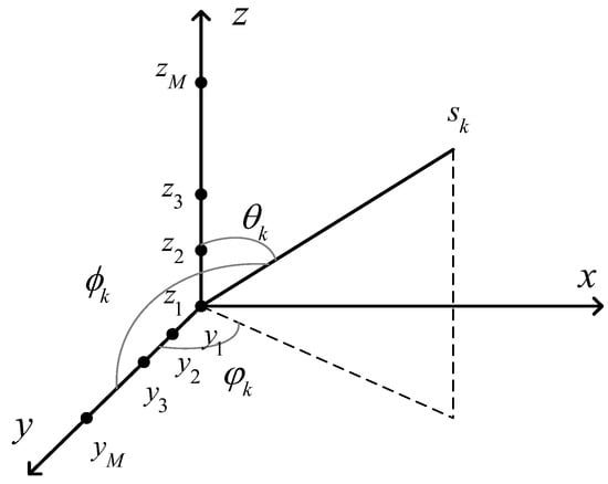
Figure 1.
Uniform L-shaped array.
Suppose that far-field narrowband sources are incident on a ULA equipped with array elements. The incoming wave direction of the incident signal is ,, is the elevation angle, is the azimuth angle and the number of snapshots is ; then, the model of the received signal of the subarray on the z-axis and y-axis can be expressed as
where and represents the array receiving signals on the z and y axes, respectively; represents the incident signal, where “” denotes the transpose operator; both and stand for the complex additive Gaussian white noise vector with zero means that are independent from the incident signal. and indicate the ideal array manifold matrix, where and satisfy the following:
In the case of multiple snapshots, the array signal models can be expressed in matrix form as follows:
At present, most signal processing methods are based on the ideal condition of the array manifold, but gain-phase errors may exist in practical applications. Therefore, considering the condition of gain-phase errors, the array signal models are expressed as
where and are the two matrices of the gain-phase error coefficients between subarray elements, and and denote the gain error and the phase error of the th array, respectively.
From the above statement, it is clear that the elevation angles and azimuth angles are estimated completely separately. However, if the elevation angles and azimuth angles are estimated separately, and then additional angle matching is performed, the overall performance of the method will be poor at low SNRs and with small snapshots. Therefore, we consider an auxiliary angle which satisfies , and then the received data can be expressed as
where , and ; based on the relationship between the three angles, the new direction vector can be expressed as , and .
3. The Proposed Method
3.1. Off-Grid Model
Let be a fixed sampling grid in the DOA range , where denotes the grid number and typically satisfies . Assuming that the source is incident to the preset grid point without bias, that is , the general array signal model with gain-phase errors can be expressed as
where is the over-complete dictionary set, and is the row sparse signal matrix obtained after extension.
Since, in actual situations, the real incident signal position is not likely to be located exactly on the preset discrete spatial grid, we introduce an off-grid model. Let represent the uniform grid with a grid interval that we set up in advance. denotes the real signal that does not belong to the set of preset discrete angles, and the first-order Taylor expansion of its steering vector can be approximated by
where represents the preset grid point closest to , , and represents the first derivative of . Expressed in matrix form, , and , in Equation (10) can be expressed as
Therefore, Equation (10) can be further updated as
Lemma 1.
For any dimensional complex vector and any dimensional complex diagonal matrix , can be obtained, where is the element on the main diagonal of the complex diagonal matrix , i.e., .
According to Lemma 1, we obtain
where , represents the dimensional identity matrix, and denotes the Kronecker product operation: , which can be obtained by summing Equations (14) and (15):
By setting , the sparse representation model of the array signal with gain-phase errors can be rewritten as
To further simplify the above equation, let .
3.2. Hierarchical Sparse Bayesian Framework
First, it is assumed that the signal received by the array is independent between different snapshots, and the noise is circular symmetric complex Gaussian white noise, which follows a Gaussian distribution. Thus, we obtain
where is the variance of noise. The complex Gaussian distributed random variable with mean and covariance obeys the probability density function of as
where “”means taking the determinant.
In this paper, the variance of noise is unknown, so it should be assumed. Since the conjugate of the inverse of the variance of the Gaussian distribution is a Gamma distribution [28], a Gamma distribution is specified for the hyperparameter , which can be described as
where and are the hyperparameters of , .
For received signals that are independent of each other, the sparse matrix is assumed to follow a Gaussian distribution with a zero mean:
Let the precision vector be a hyperparameter, which controls the estimation accuracy of the parameter to be estimated. Then, can be expressed by the Gamma prior with hyperparameters and :
For the case where the gain-phase error is unknown, and assuming that the gain phase error vector coefficients between arrays are independent of each other, the error vector distribution can also be expressed as a Gaussian distribution:
where represents the gain-phase error precision, and its distribution is described by Gamma distributions with hyperparameters and :
Then, the off-grid vector is assumed; if it follows a uniform distribution, then it can be expressed as
where
3.3. Sparse Bayesian Inference
In this subsection, a self-correcting DOA estimation method for the unknown gain-phase error is proposed that uses sparse Bayesian inference under the assumption of the unknown parameter’s distribution in the previous section.
First, we give the following equation to maximize the posterior probability:
However, since this posterior probability problem is too complicated to be solved directly, the expectation maximization (EM) algorithm is considered here to obtain a solution.
According to the received data and the parameters of the prior distribution, the posterior distribution of can be represented as
where
Both and are Gaussian functions; therefore, the posterior function of can also be expressed as a Gaussian function:
where
The next step is hyperparameter learning, which is equivalent to maximizing the posterior probability distribution of all the parameters to be estimated. In order to use Equation (28) to estimate other unknown parameters, the following likelihood can be used:
where represents , which stands for the likelihood function under the expectation with respect to the posterior of .
(1) For the noise precision . Ignoring the unrelated terms, the likelihood function of can be expressed as follows:
Setting the derivative to zero, solving for with the given updates:
(2) For the signal precision . Ignoring the unrelated terms, the likelihood function of can be expressed as follows:
Setting the derivative to zero, the th update value of can be solved as
where refers to the th row and th column elements of , and refers to the th value of .
(3) For the gain-phase error vector . Ignoring the unrelated terms, the likelihood function of can be expressed as follows:
To simplify this complicated equation, let us set
Calculating according to the above equation, the following simplification can be obtained:
For Equation (44), we calculate , and separately. For , first compute the th value of :
where is the dimensional vector with the th entry being 1 and the other entries being 0. Therefore, we can obtain
For , we can simplify it to
For , we can simplify it to
By setting , we can obtain
where
where .
(4) For the gain-phase error precision . Ignoring the independent terms, we can obtain the following likelihood function of :
Let ; then, we can obtain a newer version of the th value of :
(5) For the off-grid vector . Ignoring the independent terms, we can obtain the following likelihood function of :
Calculate according to the above equation, and similarly calculate and . First, compute the th value of :
Then, can be simplified as
For , we can simplify it to
By setting , we can obtain
where
4. Matching of Elevation Angle and Azimuth Angle
In most existing compressed sensing DOA estimation methods based on L-shaped arrays, one-dimensional DOA is used to estimate the elevation angle and azimuth angles, and then the elevation and azimuth angles are matched. The process for this kind of method is complicated and the estimation accuracy is not high. Therefore, in order to solve this problem, an auxiliary angle is proposed to realize the automatic matching of elevation and azimuth angles.
According to Equations (7) and (8), the cross-correlation covariance matrix of the two subarrays can be expressed as
where ; we then take the diagonal elements of its cross-correlation covariance matrix:
where , and represents the power of the th incident signal , which is the th diagonal element of . Equation (62) can be regarded as the received signal with angle parameter incident on a one-dimensional array of sensor elements, which satisfies the array signal model of Equation (10). Therefore, the auxiliary angle can be solved using the one-dimensional sparse Bayesian self-calibration DOA estimation method described in Section 2.
Then, according to Equation (9), the obtained by the solution is substituted into the expression of the signal received by the array:
where and represents the estimated value of the solved auxiliary angle .
Equation (63) also satisfies the array signal model of Equation (10), and can also be solved using the one-dimensional sparse Bayes self-correcting DOA estimation method in Section 2; then, the corresponding block sparse estimation results are obtained. For each “block”, the sparse signal value is recovered by searching the spectral peak, and the elevation angle corresponding to the auxiliary angle is estimated. Finally, according to the relationship between the three angles, the corresponding azimuth angle estimate can be obtained as
5. Simulation Results
Simulation experiments were conducted to compare the proposed method with the 2D-MUSIC method, OMP method and OGSBI method, so as to verify the estimation performance of the proposed method. With reference to the relevant literature, the gain-phase error of the array was assumed to conform to the following model:
where and stand for the standard deviations of gain errors and phase errors, respectively, and and are independent random variables distributed uniformly over .
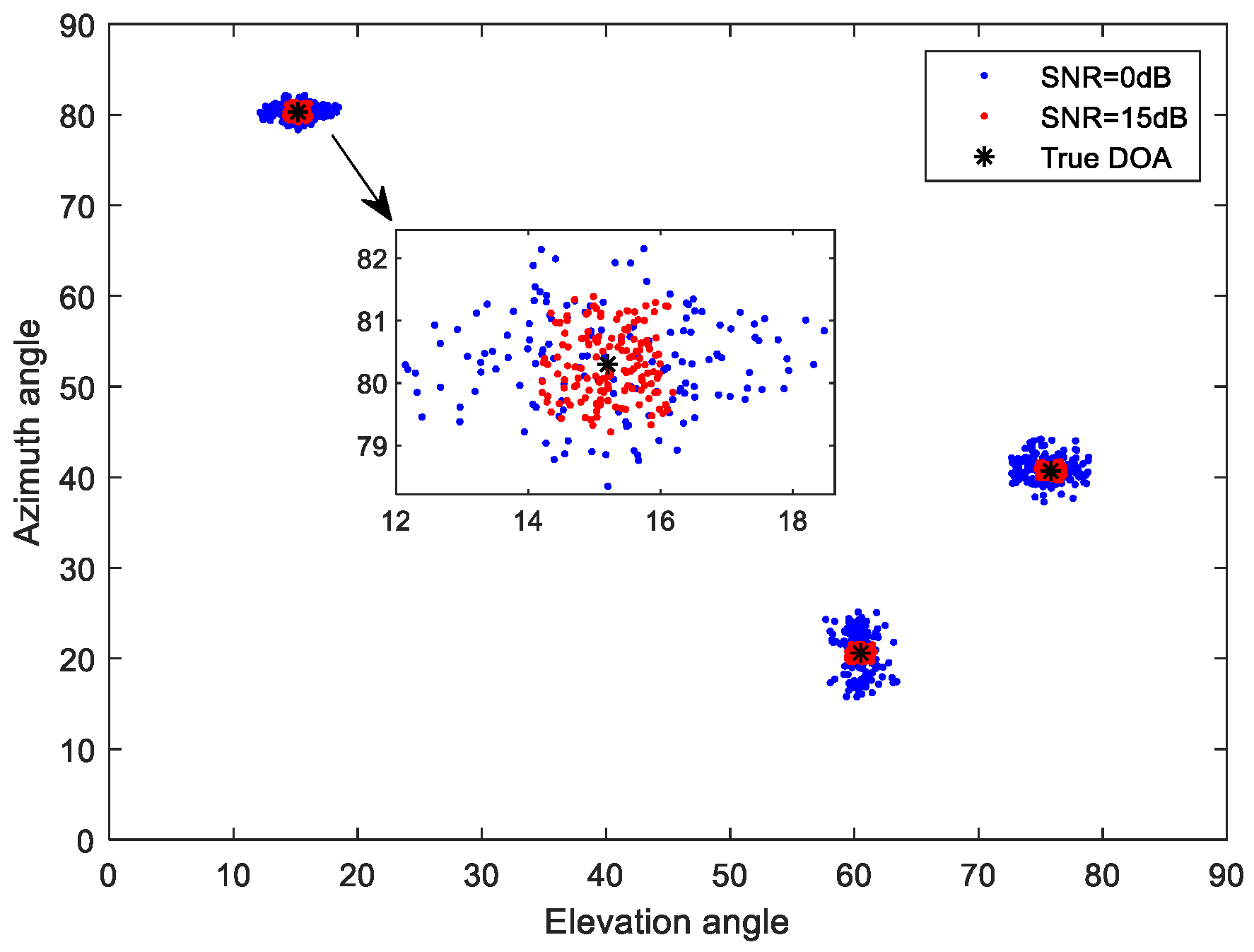
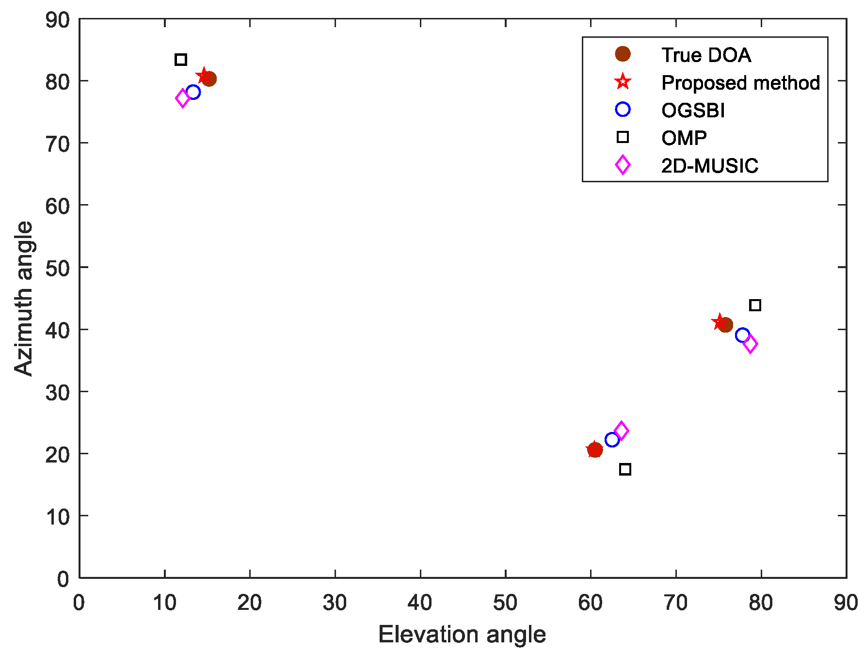
Consider a uniform L-shaped array with array elements on the subarray, with an array element spacing of half the wavelength; the wavelength was set to 0.06, and the three DOAs of the far-field narrow band signal impacting the array were , and . , the number of snapshots was 100, and the grid interval was 1°. The noise was additive white Gaussian noise. The estimation results of 150 Monte Carlo experiments under the condition of SNR = 0 dB and SNR = 15 dB are shown in Figure 2. Figure 3 shows the spatial estimation results obtained by the proposed method, 2D-MUSIC method, OMP method and OGSBI method when the SNR was 10 dB.
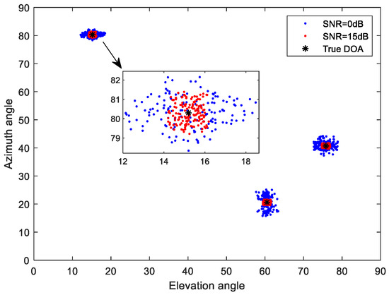
Figure 2.
Spatial estimation of the proposed method.
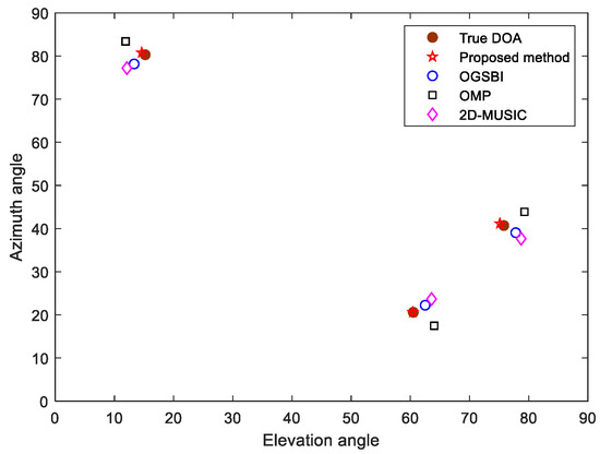
Figure 3.
Spatial estimation using different methods.
As can be seen from Figure 2, when the SNR was 15 dB, the DOA estimation result of the proposed method was close to the true direction of the incident source. When the SNR was 0 dB, although the estimation accuracy was reduced, the approximate location of the source was still effectively estimated. Compared with the other three methods, the proposed method reduced the influence of the gain-phase errors, and its estimate was the closest to the true source position (Figure 3).
The root mean square error (RMSE) was used to evaluate the estimation errors of the proposed method and the 2D-MUSIC, OMP and OGSBI methods. The number of Monte Carlo simulation experiments was set to , and the root-mean-square error of the elevation angle and the azimuth angle estimations of incident signals are defined as
where represents the estimated azimuth angle of the th signal in the th Monte Carlo simulation experiment and represents the estimated elevation angle of the th signal in the th Monte Carlo simulation experiment.
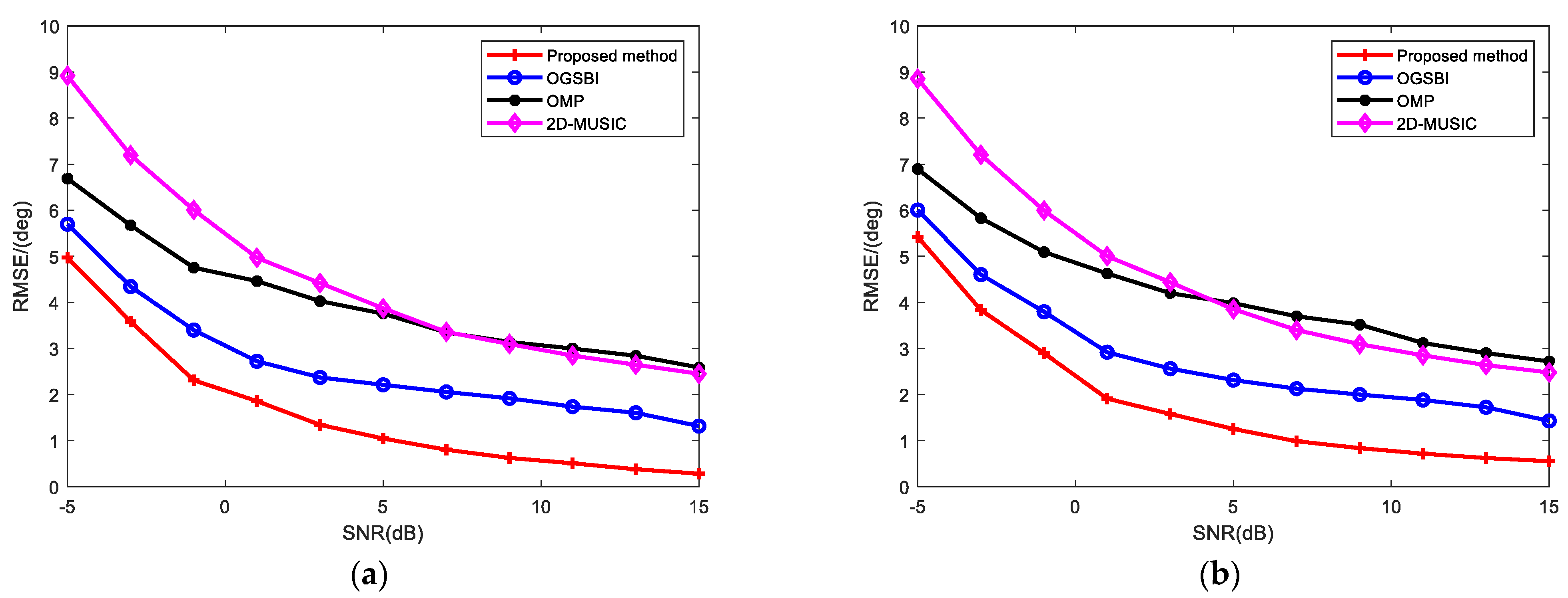
Figure 4 shows the RMSEs of the OGSBI method, OMP method, 2D-MUSIC method and the proposed method when the SNR was changed without affecting any of the other settings. It can be seen that the RMSE curves of the four methods all decreased gradually with increasing SNR. The RMSE curves of the 2D-MUSIC and OMP methods were higher and the error was large. The proposed method was superior to the other methods in this SNR interval with the lowest RMSE curve and the smallest error. When the SNR was 15 dB, not only the RMSE of the elevation angle, but also the RMSE of the azimuth angle were at the lowest values, only 0.2838 and 0.5537. This shows that when the SNR is high, the advantages of the proposed method are more obvious.
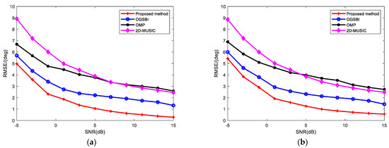
Figure 4.
RMSE vs. SNR for (a) elevation angle; (b) azimuth angle.
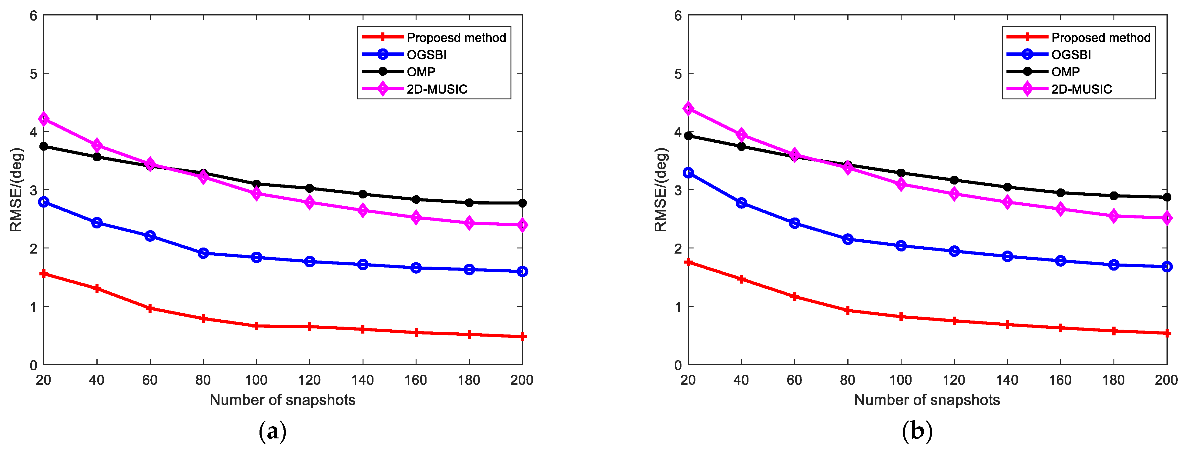
Figure 5 shows the RMSEs of the four methods when the SNR was set to 10 dB and the other experimental conditions were unchanged. The RMSEs of the four methods showed a decreasing trend with increasing number of snapshots. The RMSE curve of the proposed method was lower than that of the other three methods, and the RMSEs of the elevation and azimuth angles were only 1.5596 and 1.7965 when the number of snapshots was 20. This shows that the proposed method has the best estimation performance under different snapshot numbers compared to the other methods.
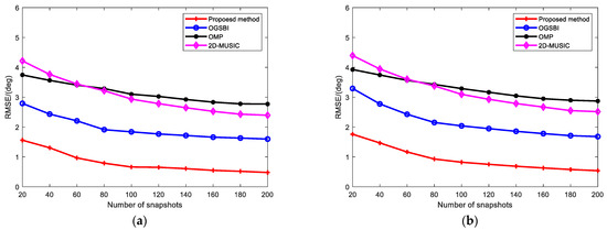
Figure 5.
RMSE vs. number of snapshots for (a) elevation angle; (b) azimuth angle.
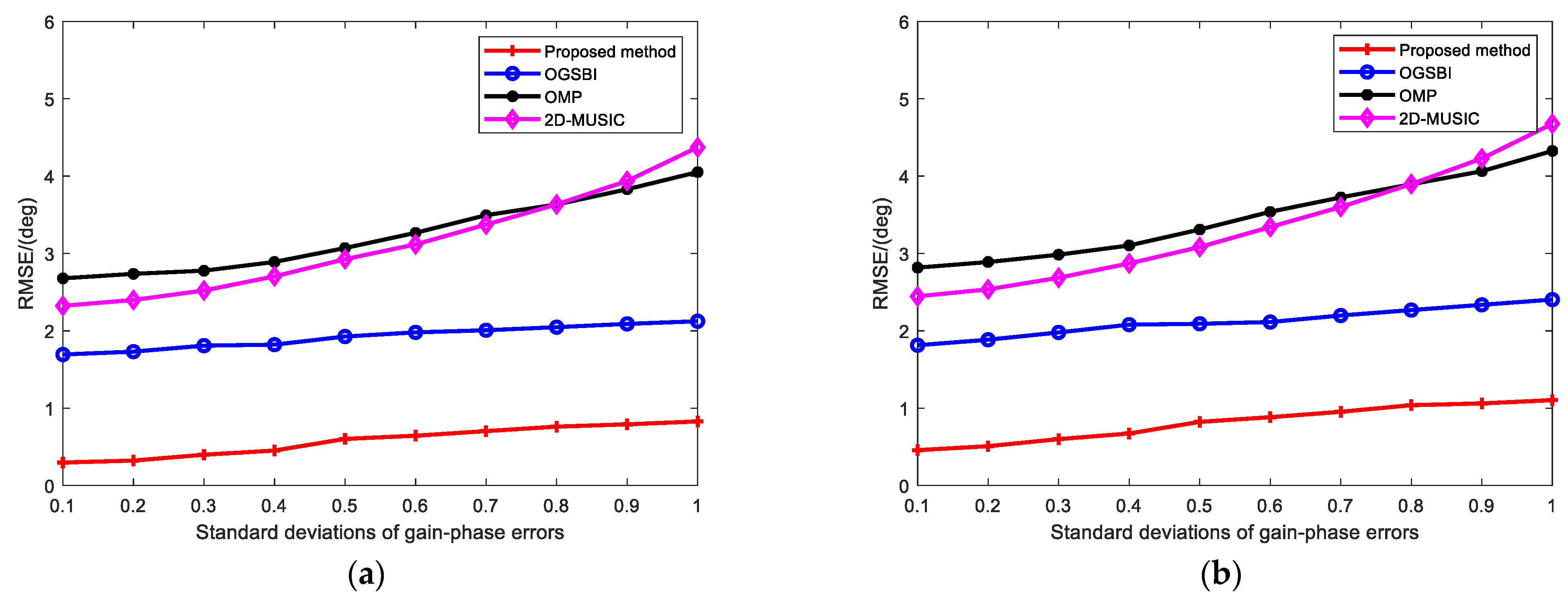
Figure 6 shows the RMSE of the four methods when, with the other experimental conditions unchanged, the SNR was set to 10 dB, the number of snapshots was 100, and the magnitude of the gain-phase error (i.e., the standard deviation coefficient of the gain-phase error) was changed. The RMSEs of the four methods increased with the increase in gain-phase errors, but the proposed method was less affected by the magnitude of the gain-phase errors, and the RMSE curve remained the lowest. The 2D-MUSIC method was significantly affected by gain-phase errors, and its RMSE fluctuated the most. This shows that, compared to other methods, the proposed method can effectively reduce the influence of gain-phase errors and has the best estimation performance.
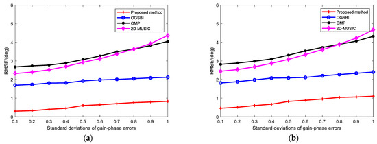
Figure 6.
RMSE vs. standard deviation of gain-phase errors for (a) elevation angle; (b) azimuth angle.
The angular resolution ability is another important index that can be used to judge the performance of DOA estimation, and the resolution ability of different methods is different. In this study, the angular resolution ability of the proposed method was evaluated from the perspective of SNR and the standard deviation coefficient of the gain-phase error. The method can identify the source position correctly, when the following conditions are met:
where is the estimate of the true azimuth angle , is the estimate of the true elevation angle , and represents the set angle error threshold, which is set to 1 here.
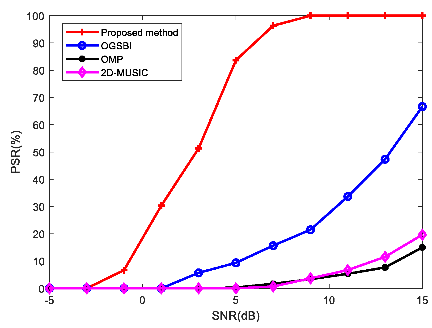
Keeping the other experimental conditions unchanged, the number of snapshots was set to 100, , and the SNR was varied. The results of the probability of successful resolution (PSR) of the OGSBI method, OMP method, 2D-MUSIC method and the proposed method are shown in Figure 7.
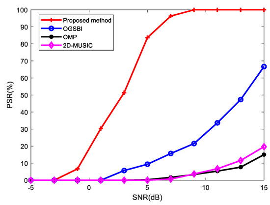
Figure 7.
PSR vs. SNR.
It can be seen from Figure 7 that the PSR of the proposed method was higher than that of the other methods in both low and high SNR scenarios. The PSR of the proposed method reached 100% when the SNR was 9 dB, while the other three methods did not reached 100% even when the SNR was 15 dB, and their success probability of resolution was low, and their resolution ability was poor. This shows that the proposed method has better angular resolution and robustness compared to the other methods under different SNR conditions.
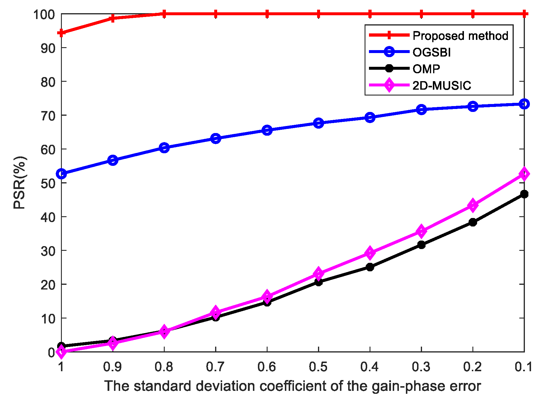
In Figure 8, the PSRs of the four methods are compared when, keeping the other experimental conditions unchanged, the number of snapshots was set to 100, the SNR was set to 15 dB, and the standard deviation coefficients of the gain-phase error and were changed. The figure shows that, in the case of large gain-phase errors, the PSRs of the other methods were low, and the OMP and 2D-MUSIC methods could not successfully predict the angles, while the PSR of the proposed method reached 66.7%. In the case of small gain-phase errors, the PSR of the proposed method reached 100%, which is obviously better than the other methods.

Figure 8.
PSR vs. standard deviation of gain-phase error.
6. Conclusions
In order to solve the problems of low accuracy and poor angular resolution caused by unknown gain-phase errors, a robust sparse Bayesian two-dimensional DOA estimation method for scenarios with gain-phase errors was proposed in this paper. To avoid the additional angle matching problem in the traditional method, the proposed method introduces an auxiliary angle to match the elevation angle and the azimuth angle. A new sparse representation model with gain-phase errors is constructed by using the diagonal elements of the cross-correlation matrix received by two submatrices, and auxiliary angles are obtained by sparse Bayes inference. By substituting in the obtained auxiliary angles, a new sparse representation model is constructed again according to the relationship between the three angles, and the corresponding block sparse estimation results are obtained. For each “block”, the corresponding DOA is obtained by searching the spectral peak. The simulation results show that the DOA estimation accuracy and angle resolution of the proposed method are superior to the OGSBL, OMP and 2D-MUSIC methods in cases where gain-phase errors exist.
Author Contributions
Methodology and writing—original draft, X.J.; writing—review and editing and supervision, X.W. (Xuhu Wang); formal analysis, Y.H.; writing—review and editing, S.H. and X.W. (Xinjie Wang); validation, Z.X. and Q.Z. All authors have read and agreed to the published version of the manuscript.
Funding
This work was funded by the National Natural Science Foundation of China under Grant 62171247, and the Shandong Provincial Natural Science Foundation of China under Grants ZR2021QF113 and ZR2022MF273.
Institutional Review Board Statement
Not applicable.
Informed Consent Statement
Not applicable.
Data Availability Statement
Data are contained within the article.
Acknowledgments
The authors would like to thank those who aided in the analysis and visualization: Gaoli Sun, Jinsong He, Honghao Feng, Lei Ding, Jianing Lu, Lei Zheng, Yuchen Wu, and Shibo Ma.
Conflicts of Interest
The authors declare no conflict of interest.
References
- Zhu, C.Q.; Fang, S.L.; Wu, Q.S.; An, L.; Luo, X.W. Robust wideband DOA estimation based on element-space data reconstruction in a multi-source environment. IEEE Access 2021, 9, 43522–43539. [Google Scholar] [CrossRef]
- Moradkhan, S.; Hosseinzadeh, S.; Zaker, R. Deep-Learning based DOA estimation in the presence of multiplicative noise. Wirel. Pers. Commun. 2022, 126, 3093–3101. [Google Scholar] [CrossRef]
- Liu, Y.; Dong, N.; Zhang, X.H.; Zhao, X.; Zhang, Y.H.; Qiu, T.S. DOA estimation for massive MIMO systems with unknown mutual coupling based on block sparse Bayesian learning. Sensors 2022, 22, 8634. [Google Scholar] [CrossRef] [PubMed]
- Wanger, M.; Park, Y.; Gerstoft, P. Gridless DOA estimation and Root-MUSIC for non-uniform linear arrays. IEEE Trans. Signal Process. 2021, 69, 2144–2157. [Google Scholar]
- Zhang, W.; Han, Y.; Jin, M.; Li, X.S. An improved ESPRIT-Like algorithm for coherent signals DOA estimation. IEEE Commun. Lett. 2020, 24, 339–343. [Google Scholar] [CrossRef]
- Jiang, Z.M.; Zhang, P.C.; Rihan, M.; Huang, L.; Zhang, J.H. Maximum likelihood approach to DOA estimation using lens antenna array. EURASIP J. Wirel. Commun. Netw. 2019, 2019, 242. [Google Scholar] [CrossRef]
- Meller, M.; Stawiarski, K. On DOA estimation for rotating arrays using stochastic maximum Likelihood approach. IEEE Trans. Signal Process. 2020, 68, 5219–5229. [Google Scholar] [CrossRef]
- Zuo, M.; Xie, S.G.; Zhang, X.; Yang, M.L. DOA estimation based on weighted l1-norm sparse representation for low SNR scenarios. Sensors 2021, 21, 4614. [Google Scholar] [CrossRef]
- Liu, L.T.; Rao, Z.J. An adaptive Lp norm minimization algorithm for direction of arrival estimation. Remote Sens. 2022, 14, 766. [Google Scholar] [CrossRef]
- Needell, D.; Tropp, J.A. CoSaMP: Iterative Signal Recovery from Incomplete and Inaccurate Samples. Commun. ACM 2010, 53, 93–100. [Google Scholar] [CrossRef]
- Keyvan, A.; Vahid, M.S.; Behrouz, M. High-precision OMP-based direction of arrival estimation scheme for hybrid non-uniform array. IEEE Commun. Lett. 2020, 24, 354–357. [Google Scholar]
- Babacan, S.D.; Molina, R.; Katsaggelos, A.K. Bayesian compressive sensing using laplace priors. IEEE Trans. Image Process. 2010, 19, 53–63. [Google Scholar] [CrossRef] [PubMed]
- Yang, Z.; Xie, L.H.; Zhang, C.S. Off-grid direction of arrival estimation using sparse Bayesian inference. IEEE Trans. Signal Process. 2013, 61, 38–43. [Google Scholar] [CrossRef]
- Dai, J.S.; Bao, X.; Xu, W.C.; Chang, C.Q. Root sparse Bayesian learning for off-grid DOA estimation. IEEE Signal Process. Lett. 2017, 24, 46–50. [Google Scholar] [CrossRef]
- Huang, H.P.; So, H.C.; Zoubir, A.M. Off-grid direction-of-arrival estimation using second-order Taylor approximation. Signal Process. 2022, 196, 108513–108519. [Google Scholar] [CrossRef]
- Liu, D.H.; Zhao, Y.B. Real-valued sparse Bayesian learning algorithm for off-grid DOA estimation in the beamspace. Digit. Signal Process. 2022, 121, 103322–103328. [Google Scholar] [CrossRef]
- Zeng, H.W.; Yue, H.; Cao, J.K.; Zhang, X.F. Real-valued direct position determination of quasi-stationary signals for nested arrays: Khatri–Rao Subspace and Unitary Transformation. Sensors 2022, 22, 4209. [Google Scholar] [CrossRef]
- Zhang, Y.H.; Yang, Y.X.; Yang, L. Off-grid DOA estimation through variational Bayesian inference in colored noise environment. Digit. Signal Process. 2021, 111, 102967–102981. [Google Scholar] [CrossRef]
- Wang, P.Y.; Yang, H.C.; Ye, Z.F. An off-grid wideband DOA estimation method with the variational Bayes expectation-maximization framework. Signal Process. 2022, 193, 108423–108430. [Google Scholar] [CrossRef]
- Wang, H.F.; Wang, X.P.; Huang, M.X.; Wan, L.T. A novel variational SBL approach for off-grid DOA detection under nonuniform noise. Digit. Signal Process. 2022, 128, 103622–103630. [Google Scholar] [CrossRef]
- Liu, Z.Y.; Liu, Y.; Long, X.D.; Zhang, Y.H.; Qiu, T.S. Improved block sparse Bayesian learning based DOA estimation for massive MIMO systems. AEUE-Int. J. Electron. Commun. 2023, 166, 154666–154676. [Google Scholar] [CrossRef]
- Zhou, H.; Wen, B.Y. Calibration of antenna pattern and phase errors of a cross-loop/monopole antenna array in high-frequency surface wave radars. IET Radar Sonar Navig. 2014, 8, 407–414. [Google Scholar] [CrossRef]
- Wang, Z.S.; Xie, W.; Wan, Q. DOA estimation of multipath signals in the presence of gain-phase errors using an auxiliary source. IEEJ Trans. Electr. Electron. Eng. 2019, 14, 1114–1121. [Google Scholar] [CrossRef]
- Tian, Y.; Shi, J.X.; Yue, H.; Rong, X.L. Calibrating nested sensor arrays for DOA estimation utilizing continuous multiplication operator. Signal Process. 2020, 176, 107674–107684. [Google Scholar] [CrossRef]
- Peng, W.C.; Guo, C.J.; Wang, M.; Gao, Y.T. An improved gain-phase error self-calibration method for robust DOA estimation. Int. J. Microw. Wirel. Technol. 2019, 11, 105–113. [Google Scholar] [CrossRef]
- Wei, Z.Y.; Wang, W.; Dong, F.W.; Liu, P. Self-calibration algorithm with gain-phase errors array for robust DOA estimation. Prog. Electromagn. Res. M 2021, 99, 1–12. [Google Scholar] [CrossRef]
- Gong, Q.S.; Ren, S.W.; Zhong, S.N.; Wang, W.J. DOA estimation using sparse array with gain-phase error based on a novel atomic norm. Digit. Signal Process. 2022, 120, 103266–103279. [Google Scholar] [CrossRef]
- Ji, S.H.; Xue, Y.; Carin, L. Bayesian compressive sensing. IEEE Trans. Signal Process. 2008, 56, 2346–2356. [Google Scholar] [CrossRef]

Disclaimer/Publisher’s Note: The statements, opinions and data contained in all publications are solely those of the individual author(s) and contributor(s) and not of MDPI and/or the editor(s). MDPI and/or the editor(s) disclaim responsibility for any injury to people or property resulting from any ideas, methods, instructions or products referred to in the content. |
© 2023 by the authors. Licensee MDPI, Basel, Switzerland. This article is an open access article distributed under the terms and conditions of the Creative Commons Attribution (CC BY) license (https://creativecommons.org/licenses/by/4.0/).