
Maritime Infrared Small Target Detection Based on the Appearance Stable Isotropy Measure in Heavy Sea Clutter Environments
 , , , ,
  and
and
Abstract
:1. Introduction
1.1. Related Work
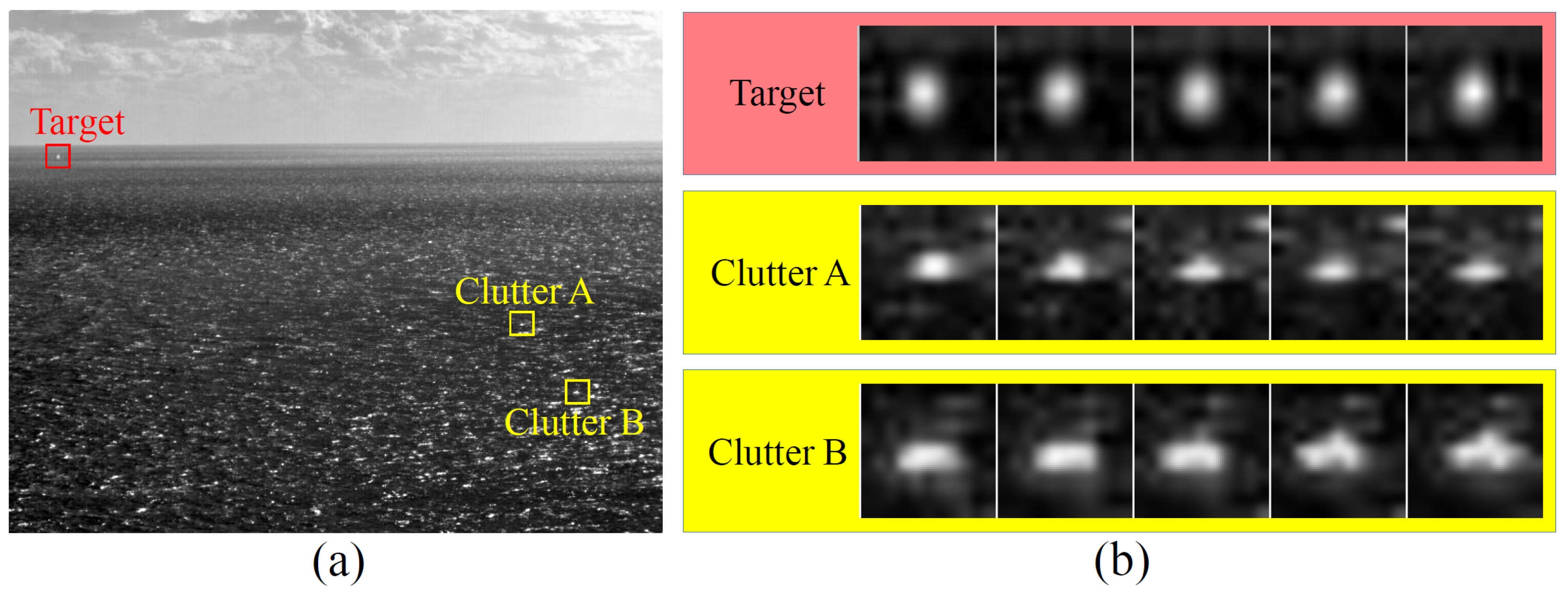
1.2. Motivation
- (1)
- The Gradient Histogram Equalization Measure (GHEM) is proposed to effectively characterize the spatial isotropy of local regions. It aids in distinguishing small targets from anisotropic clutter.
- (2)
- The Local Optical Flow Consistency Measure (LOFCM) is proposed to assess the temporal stability of local regions. It facilitates the differentiation of small targets from isotropic clutter.
- (3)
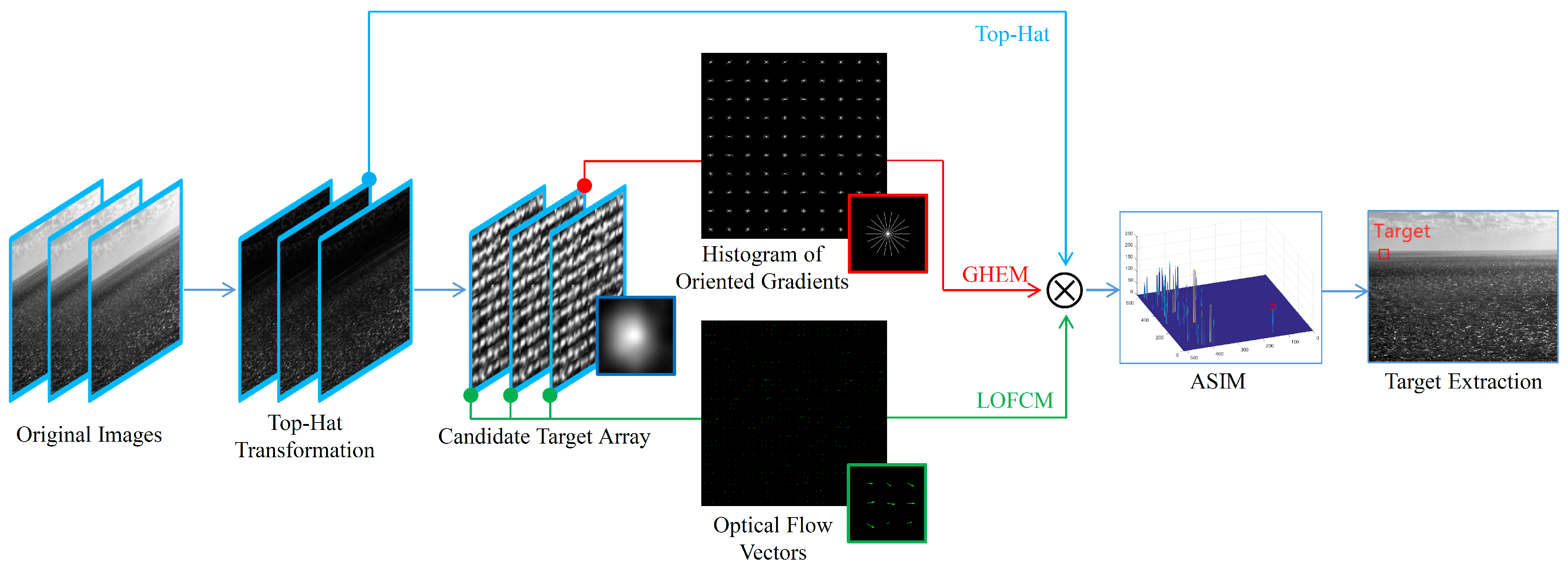
- By combining GHEM, LOFCM, and Top-Hat, ASIM is developed as a comprehensive characteristic for distinguishing between small targets and different types of sea clutter. We also construct an algorithm based on ASIM for IR small target detection in heavy sea clutter environments.
- (4)
- Experimental results validate the superior performance of the proposed method compared to the baseline methods in heavy sea clutter environments.
2. Proposed Method
2.1. Candidate Target Extraction
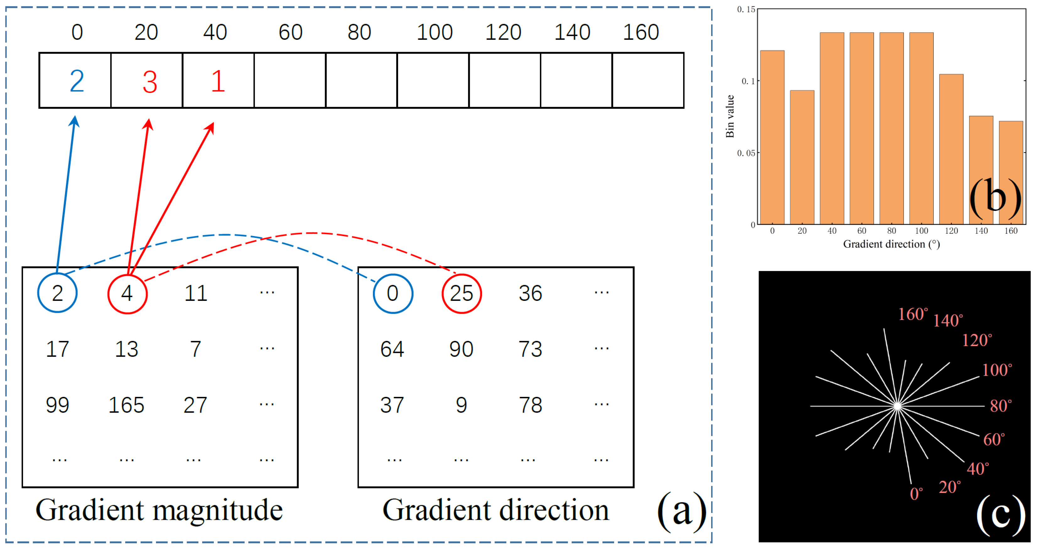
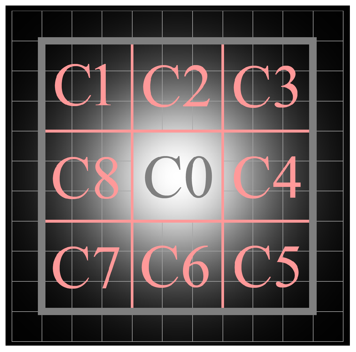
2.2. Gradient Histogram Equalization Measure (GHEM)
2.3. Local Optical Flow Consistency Measure (LOFCM)
- (1)
- Brightness constancy: The gray value of a pixel does not change over time.
- (2)
- Small motion: The displacement of a pixel is small, and the passage of time cannot cause drastic changes in the pixel position.
- (3)
- Local spatial consistency: The relative positions of neighboring pixels do not change.
2.4. Appearance Stable Isotropy Measure
| Algorithm 1 ASIM. |
| Input: frame , t, and |
Output: ASIM image
|
3. Experiments
3.1. Evaluation Metrics
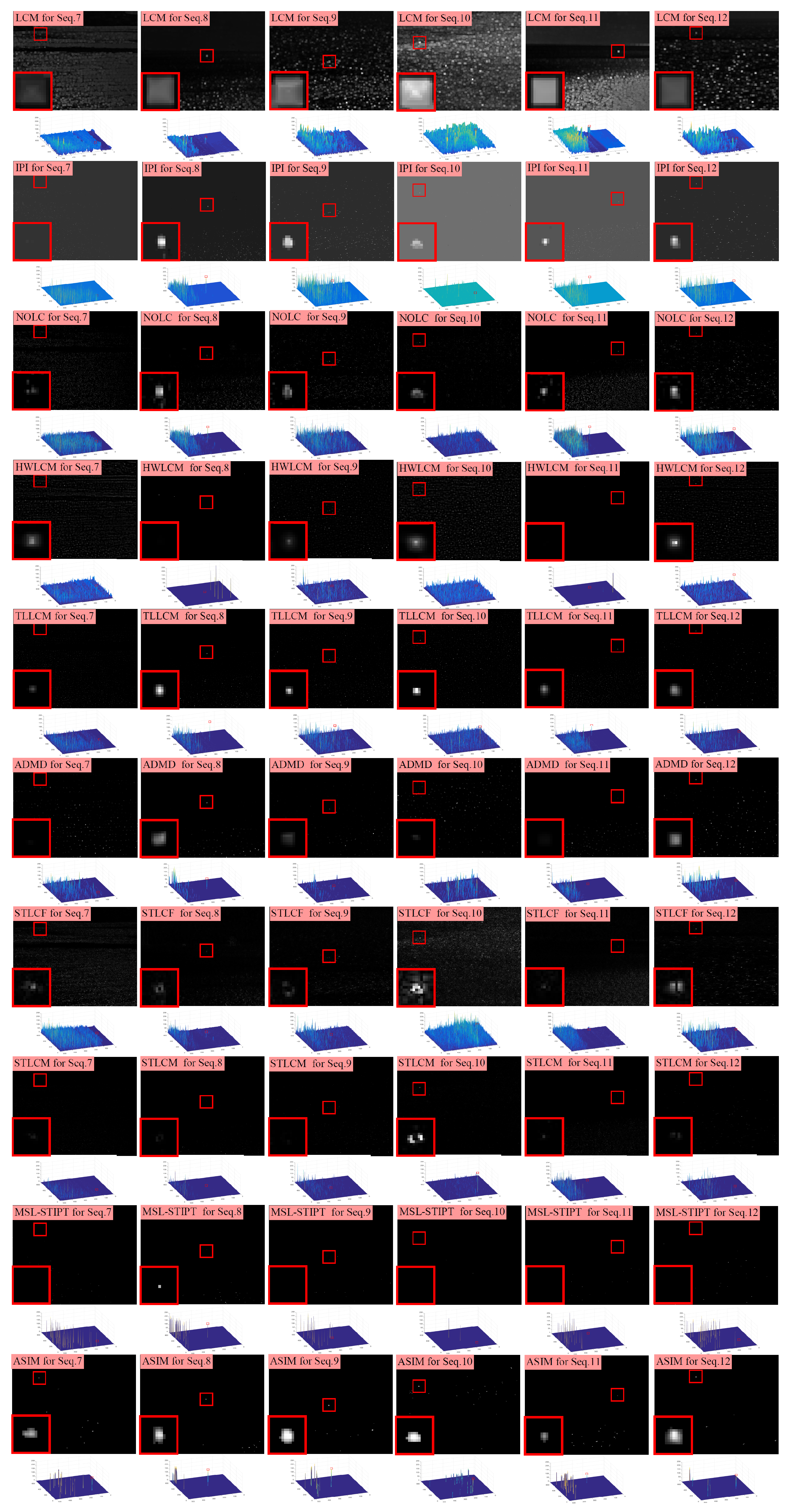
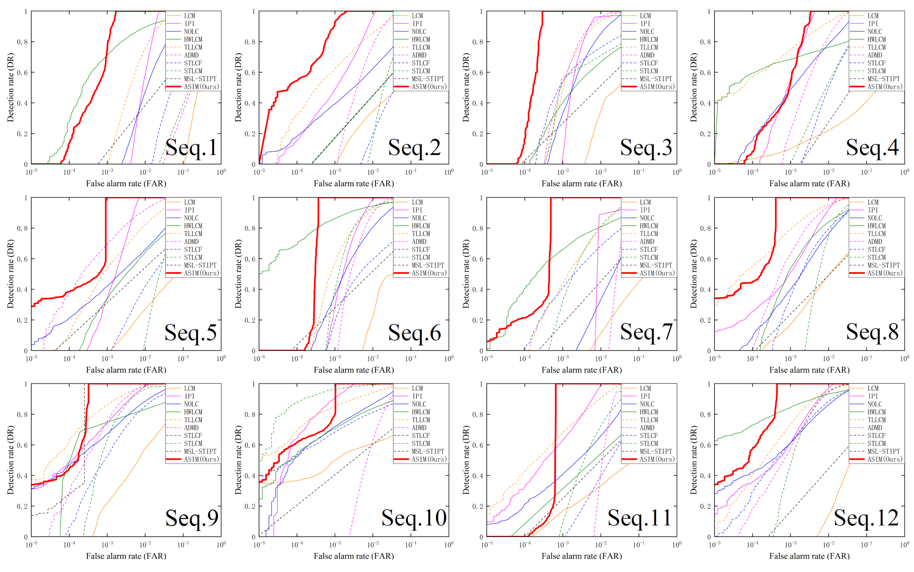
3.2. Experimental Results
4. Conclusions
Author Contributions
Funding
Institutional Review Board Statement
Informed Consent Statement
Data Availability Statement
Conflicts of Interest
References
- Zhang, H.; Qian, W.; Wan, M.; Zhang, K.; Wang, F.; Kong, X.; Chen, Q.; Lu, D. Robust noise hybrid active contour model for infrared image segmentation using orientation column filters. J. Mod. Opt. 2023, 70, 483–502. [Google Scholar] [CrossRef]
- Lu, Y.; Dong, L.; Zhang, T.; Xu, W. A robust detection algorithm for infrared maritime small and dim targets. Sensors 2020, 20, 1237. [Google Scholar] [CrossRef]
- Tom, V.T.; Peli, T.; Leung, M.; Bondaryk, J.E. Morphology-based algorithm for point target detection in infrared backgrounds. In Proceedings of the Signal and Data Processing of Small Targets 1993, International Society for Optics and Photonics, Orlando, FL, USA, 12–14 April 1993; Volume 1954, pp. 2–11. [Google Scholar]
- Deshpande, S.D.; Er, M.H.; Venkateswarlu, R.; Chan, P. Max-mean and max-median filters for detection of small targets. In Proceedings of the Signal and Data Processing of Small Targets 1999, International Society for Optics and Photonics, Denver, CO, USA, 19–23 July 1999; Volume 3809, pp. 74–83. [Google Scholar]
- Hadhoud, M.M.; Thomas, D.W. The two-dimensional adaptive LMS (TDLMS) algorithm. IEEE Trans. Circuits Syst. 1988, 35, 485–494. [Google Scholar] [CrossRef]
- Wang, B.; Dong, L.; Zhao, M.; Xu, W. Fast infrared maritime target detection: Binarization via histogram curve transformation. Infrared Phys. Technol. 2017, 83, 32–44. [Google Scholar] [CrossRef]
- Bai, X.; Zhou, F.; Xie, Y. New class of top-hat transformation to enhance infrared small targets. J. Electron. Imaging 2008, 17, 030501. [Google Scholar] [CrossRef]
- Zhang, Y.; Li, L.; Xin, Y. Infrared small target detection based on adaptive double-layer TDLMS filter. Acta Photonica Sin. 2019, 48, 0910001. [Google Scholar] [CrossRef]
- Wang, X.; Lv, G.; Xu, L. Infrared dim target detection based on visual attention. Infrared Phys. Technol. 2012, 55, 513–521. [Google Scholar] [CrossRef]
- Kim, S.; Yang, Y.; Lee, J.; Park, Y. Small target detection utilizing robust methods of the human visual system for IRST. J. Infrared Millim. Terahertz Waves 2009, 30, 994–1011. [Google Scholar] [CrossRef]
- Wang, X.; Lu, R.; Bi, H.; Li, Y. An Infrared Small Target Detection Method Based on Attention Mechanism. Sensors 2023, 23, 8608. [Google Scholar] [CrossRef]
- Moradi, S.; Moallem, P.; Sabahi, M.F. A false-alarm aware methodology to develop robust and efficient multi-scale infrared small target detection algorithm. Infrared Phys. Technol. 2018, 89, 387–397. [Google Scholar] [CrossRef]
- Aghaziyarati, S.; Moradi, S.; Talebi, H. Small infrared target detection using absolute average difference weighted by cumulative directional derivatives. Infrared Phys. Technol. 2019, 101, 78–87. [Google Scholar] [CrossRef]
- Moradi, S.; Moallem, P.; Sabahi, M.F. Fast and robust small infrared target detection using absolute directional mean difference algorithm - ScienceDirect. Signal Process. 2020, 177, 107727. [Google Scholar] [CrossRef]
- Chen, C.P.; Li, H.; Wei, Y.; Xia, T.; Tang, Y.Y. A local contrast method for small infrared target detection. IEEE Trans. Geosci. Remote Sens. 2013, 52, 574–581. [Google Scholar] [CrossRef]
- Han, J.; Ma, Y.; Zhou, B.; Fan, F.; Liang, K.; Fang, Y. A robust infrared small target detection algorithm based on human visual system. IEEE Geosci. Remote Sens. Lett. 2014, 11, 2168–2172. [Google Scholar]
- Qin, Y.; Li, B. Effective infrared small target detection utilizing a novel local contrast method. IEEE Geosci. Remote Sens. Lett. 2016, 13, 1890–1894. [Google Scholar] [CrossRef]
- Wei, Y.; You, X.; Li, H. Multiscale patch-based contrast measure for small infrared target detection. Pattern Recognit. 2016, 58, 216–226. [Google Scholar] [CrossRef]
- Han, J.; Moradi, S.; Faramarzi, I.; Liu, C.; Zhao, Q. A Local Contrast Method for Infrared Small-Target Detection Utilizing a Tri-Layer Window. IEEE Geosci. Remote Sens. Lett. 2019, 17, 1822–1826. [Google Scholar] [CrossRef]
- Du, P.; Hamdulla, A. Infrared small target detection using homogeneity-weighted local contrast measure. IEEE Geosci. Remote Sens. Lett. 2019, 17, 514–518. [Google Scholar] [CrossRef]
- Han, J.; Moradi, S.; Faramarzi, I.; Zhang, H.; Zhao, Q.; Zhang, X.; Li, N. Infrared small target detection based on the weighted strengthened local contrast measure. IEEE Geosci. Remote Sens. Lett. 2020, 18, 1670–1674. [Google Scholar] [CrossRef]
- Deng, L.; Zhu, H.; Tao, C.; Wei, Y. Infrared moving point target detection based on spatial–temporal local contrast filter. Infrared Phys. Technol. 2016, 76, 168–173. [Google Scholar] [CrossRef]
- Zhao, B.; Xiao, S.; Lu, H.; Wu, D. Spatial-temporal local contrast for moving point target detection in space-based infrared imaging system. Infrared Phys. Technol. 2018, 95, 53–60. [Google Scholar] [CrossRef]
- Du, P.; Hamdulla, A. Infrared moving small-target detection using spatial–temporal local difference measure. IEEE Geosci. Remote Sens. Lett. 2019, 17, 1817–1821. [Google Scholar] [CrossRef]
- Pang, D.; Shan, T.; Ma, P.; Li, W.; Liu, S.; Tao, R. A novel spatiotemporal saliency method for low-altitude slow small infrared target detection. IEEE Geosci. Remote Sens. Lett. 2021, 19, 1–5. [Google Scholar] [CrossRef]
- Gao, C.; Meng, D.; Yang, Y.; Wang, Y.; Zhou, X.; Hauptmann, A.G. Infrared patch-image model for small target detection in a single image. IEEE Trans. Image Process. 2013, 22, 4996–5009. [Google Scholar] [CrossRef]
- Dai, Y.; Wu, Y.; Song, Y. Infrared small target and background separation via column-wise weighted robust principal component analysis. Infrared Phys. Technol. 2016, 77, 421–430. [Google Scholar] [CrossRef]
- Dai, Y.; Wu, Y.; Song, Y.; Guo, J. Non-negative infrared patch-image model: Robust target-background separation via partial sum minimization of singular values. Infrared Phys. Technol. 2017, 81, 182–194. [Google Scholar] [CrossRef]
- Zhang, T.; Wu, H.; Liu, Y.; Peng, L.; Yang, C.; Peng, Z. Infrared small target detection based on non-convex optimization with Lp-norm constraint. Remote Sens. 2019, 11, 559. [Google Scholar] [CrossRef]
- He, Y.; Li, M.; Zhang, J.; An, Q. Small infrared target detection based on low-rank and sparse representation. Infrared Phys. Technol. 2015, 68, 98–109. [Google Scholar] [CrossRef]
- Wang, X.; Peng, Z.; Kong, D.; He, Y. Infrared dim and small target detection based on stable multisubspace learning in heterogeneous scene. IEEE Trans. Geosci. Remote Sens. 2017, 55, 5481–5493. [Google Scholar] [CrossRef]
- Dai, Y.; Wu, Y. Reweighted infrared patch-tensor model with both nonlocal and local priors for single-frame small target detection. IEEE J. Sel. Top. Appl. Earth Obs. Remote Sens. 2017, 10, 3752–3767. [Google Scholar] [CrossRef]
- Zhang, L.; Peng, Z. Infrared Small Target Detection Based on Partial Sum of the Tensor Nuclear Norm. Remote Sens. 2019, 11, 382. [Google Scholar] [CrossRef]
- Guan, X.; Zhang, L.; Huang, S.; Peng, Z. Infrared small target detection via non-convex tensor rank surrogate joint local contrast energy. Remote Sens. 2020, 12, 1520. [Google Scholar] [CrossRef]
- Sun, Y.; Yang, J.; An, W. Infrared Dim and Small Target Detection via Multiple Subspace Learning and Spatial-Temporal Patch-Tensor Model. IEEE Trans. Geosci. Remote Sens. 2020, 59, 3737–3752. [Google Scholar] [CrossRef]
- Liu, H.K.; Zhang, L.; Huang, H. Small Target Detection in Infrared Videos Based on Spatio-Temporal Tensor Model. IEEE Trans. Geosci. Remote Sens. 2020, 58, 8689–8700. [Google Scholar] [CrossRef]
- Pang, D.; Ma, P.; Shan, T.; Li, W.; Tao, R.; Ma, Y.; Wang, T. STTM-SFR: Spatial–Temporal Tensor Modeling with Saliency Filter Regularization for Infrared Small Target Detection. IEEE Trans. Geosci. Remote Sens. 2022, 60, 1–18. [Google Scholar] [CrossRef]
- Zhao, M.; Cheng, L.; Yang, X.; Feng, P.; Liu, L.; Wu, N. TBC-Net: A real-time detector for infrared small target detection using semantic constraint. arXiv 2019, arXiv:2001.05852. [Google Scholar]
- Li, B.; Xiao, C.; Wang, L.; Wang, Y.; Lin, Z.; Li, M.; An, W.; Guo, Y. Dense nested attention network for infrared small target detection. arXiv 2021, arXiv:2106.00487. [Google Scholar] [CrossRef]
- Liu, F.; Gao, C.; Chen, F.; Meng, D.; Zuo, W.; Gao, X. Infrared Small and Dim Target Detection with Transformer Under Complex Backgrounds. IEEE Trans. Image Process. 2023, 32, 5921–5932. [Google Scholar] [CrossRef]
- Chen, G.; Wang, W.; Tan, S. Irstformer: A hierarchical vision transformer for infrared small target detection. Remote Sens. 2022, 14, 3258. [Google Scholar] [CrossRef]
- Dai, Y.; Wu, Y.; Zhou, F.; Barnard, K. Attentional local contrast networks for infrared small target detection. IEEE Trans. Geosci. Remote Sens. 2021, 59, 9813–9824. [Google Scholar] [CrossRef]
- Xin, J.; Cao, X.; Xiao, H.; Liu, T.; Liu, R.; Xin, Y. Infrared Small Target Detection Based on Multiscale Kurtosis Map Fusion and Optical Flow Method. Sensors 2023, 23, 1660. [Google Scholar] [CrossRef] [PubMed]


| Sequence | Image Size | Frame Number | Target Type | Target Size |
|---|---|---|---|---|
| Seq.1 | 512 × 640 | 1000 | Signal light | 5 × 4 |
| Seq.2 | 512 × 640 | 1000 | Signal light | 3 × 3 |
| Seq.3 | 512 × 640 | 1000 | Ship | 9 × 9 |
| Seq.4 | 512 × 640 | 97 | Ship | 9 × 7 |
| Seq.5 | 512 × 640 | 400 | Signal light | 5 × 5 |
| Seq.6 | 512 × 640 | 500 | Ship | 7 × 7 |
| Seq.7 | 512 × 640 | 1000 | Ship | 5 × 5 |
| Seq.8 | 512 × 640 | 1000 | Signal light | 7 × 7 |
| Seq.9 | 512 × 640 | 1000 | Signal light | 6 × 5 |
| Seq.10 | 512 × 640 | 500 | Ship | 5 × 6 |
| Seq.11 | 512 × 640 | 500 | Signal light | 4 × 4 |
| Seq.12 | 512 × 640 | 500 | Ship | 6 × 6 |
| Sequence | LCM | IPI | NOLC | HWLCM | TLLCM | ADMD | STLCF | STLCM | MSL-STIPT | ASIM (Ours) | |
|---|---|---|---|---|---|---|---|---|---|---|---|
| BSF | Seq.1 | 2.35 | 5.9603 | 4.6786 | 11.5765 | 13.2104 | 16.4142 | 13.1323 | 17.1572 | 14.2337 | 19.0300 |
| Seq.2 | 4.3029 | 11.4957 | 3.9490 | 18.1301 | 12.8368 | 14.6817 | 7.9277 | 12.5154 | 22.4095 | 28.1576 | |
| Seq.3 | 4.4258 | 15.3305 | 11.1006 | 4.7119 | 14.8072 | 16.3769 | 19.2110 | 32.4433 | 19.3694 | 25.6798 | |
| Seq.4 | 0.9816 | 10.8962 | 5.2172 | 1.5451 | 5.2782 | 7.6194 | 3.6652 | 7.3866 | 5.2973 | 11.2543 | |
| Seq.5 | 4.2431 | 13.1191 | 3.6601 | 6.6224 | 19.0589 | 14.3481 | 5.2402 | 26.9579 | 36.2472 | 20.5585 | |
| Seq.6 | 4.0975 | 18.4130 | 9.9744 | 11.6162 | 19.1893 | 16.3994 | 10.5474 | 34.6185 | 32.4306 | 35.1543 | |
| Seq.7 | 3.3625 | 12.1870 | 4.4644 | 6.9145 | 13.1137 | 11.9082 | 5.0353 | 17.9317 | 15.4038 | 21.3181 | |
| Seq.8 | 1.5828 | 3.9114 | 3.4861 | 6.4551 | 6.6746 | 13.0041 | 6.3620 | 15.2050 | 14.8925 | 18.6672 | |
| Seq.9 | 4.3457 | 9.3311 | 5.9340 | 26.0391 | 12.5617 | 13.7088 | 11.3957 | 31.7395 | 15.6627 | 36.1225 | |
| Seq.10 | 1.1671 | 20.0762 | 6.2541 | 3.1570 | 5.4764 | 5.2878 | 1.7990 | 16.1800 | 40.0401 | 17.3463 | |
| Seq.11 | 1.1776 | 8.1043 | 2.7801 | 46.4676 | 9.3482 | 11.5604 | 4.5328 | 10.0845 | 14.8832 | 18.8061 | |
| Seq.12 | 2.9323 | 8.6763 | 5.9026 | 8.5013 | 14.5613 | 10.3476 | 8.5029 | 19.9019 | 17.4160 | 24.6129 | |
| SCRG | Seq.1 | 1.3695 | 11,297.0 | 15,147.0 | 5.0528 | 20.1239 | 0.7885 | 1.7908 | 11.7536 | 0.0028 | 19,515.0 |
| Seq.2 | 0.7327 | 6.6738 | 1.9079 | 2.9436 | 3.0579 | 16.5467 | 2.9956 | 5.3132 | 0.00097 | 70,620.0 | |
| Seq.3 | 1.2000 | 4.7764 | 2.9948 | 1.2734 | 4.1211 | 2929.9 | 0.7823 | 7.6465 | 0.0082 | 11,631.0 | |
| Seq.4 | 0.9025 | 2.0318 | 1.8720 | 1.6600 | 103.5336 | 4017.0 | 33.9769 | 29.6237 | 0.00034 | 9268.8 | |
| Seq.5 | 1.3870 | 19,649.0 | 3.9910 | 2.5819 | 6.7425 | 683.2696 | 4.5386 | 18.0894 | 0.0044 | 57,204.0 | |
| Seq.6 | 2.7673 | 3924.2 | 21.6796 | 9.2779 | 59.9930 | 2897.8 | 0.6596 | 50.1290 | 0.9172 | 7477.0 | |
| Seq.7 | 0.9780 | 1756.7 | 3.0760 | 4.6140 | 9.5489 | 1.6425 | 5.4671 | 20.5076 | 0.2858 | 55,392.0 | |
| Seq.8 | 0.7010 | 1.1465 | 1.2271 | 1.4607 | 2.5313 | 1315.8 | 1.0593 | 0.2334 | 0.7537 | 39,234.0 | |
| Seq.9 | 3.5557 | 9.0137 | 2.9227 | 5.1908 | 32.2832 | 12,069.0 | 3.0763 | 8.4399 | 16,002.0 | 20,609.0 | |
| Seq.10 | 1.5822 | 83.3607 | 5.7312 | 4.9129 | 12.4931 | 53.2729 | 4.8203 | 95.2062 | 0.5678 | 78,652.0 | |
| Seq.11 | 2.5551 | 8366.6 | 3.3482 | 5.2843 | 48.1007 | 570.8405 | 2.4935 | 43.9950 | 0.0759 | 7859.3 | |
| Seq.12 | 2.3255 | 18.5972 | 3.5414 | 5.9537 | 6.7523 | 9164.9 | 2.9079 | 14.6723 | 0.0540 | 7665.2 |
| Sequence | LCM | IPI | NOLC | HWLCM | TLLCM | ADMD | STLCF | STLCM | MSL-STIPT | ASIM (Ours) |
|---|---|---|---|---|---|---|---|---|---|---|
| Seq.1 | 0 | 0 | 0 | 0.7150 | 0 | 0 | 0 | 0 | 0.0739 | 0.7475 |
| Seq.2 | 0 | 0.4943 | 0.3973 | 0.1650 | 0.6295 | 0 | 0 | 0 | 0.1684 | 0.9201 |
| Seq.3 | 0 | 0.0724 | 0.3452 | 0.4049 | 0.5003 | 0.5415 | 0.5607 | 0.6622 | 0.2714 | 1 |
| Seq.4 | 0.1029 | 0.5633 | 0.4900 | 0.6892 | 0.7477 | 0.2229 | 0 | 0.0316 | 0 | 0.5379 |
| Seq.5 | 0 | 0.3437 | 0.4234 | 0.3393 | 0.5350 | 0.6957 | 0 | 0 | 0.3231 | 1 |
| Seq.6 | 0 | 0.2956 | 0.3626 | 0.8668 | 0.5800 | 0 | 0.1935 | 0.4197 | 0.2814 | 1 |
| Seq.7 | 0 | 0 | 0 | 0.6627 | 0.4506 | 0 | 0.4121 | 0.3474 | 0.1681 | 1 |
| Seq.8 | 0.1716 | 0.5123 | 0.4016 | 0.5342 | 0.7925 | 0.6323 | 0.3535 | 0 | 0.2359 | 1 |
| Seq.9 | 0.2210 | 0.7423 | 0.6756 | 1 | 0.8600 | 0.7581 | 0.5324 | 0.6448 | 1 | 1 |
| Seq.10 | 0.5016 | 0.9114 | 0.7225 | 0.7100 | 0.8574 | 0 | 0.6861 | 0.9682 | 0.4055 | 0.9951 |
| Seq.11 | 0.1773 | 0.6337 | 0.4169 | 0.3200 | 0.6825 | 0 | 0 | 0.0966 | 0.2575 | 1 |
| Seq.12 | 0 | 0.6149 | 0.6130 | 0.8457 | 0.7375 | 0.5780 | 0.6130 | 0.4835 | 0.1723 | 1 |
| Sequence | LCM | IPI | NOLC | HWLCM | TLLCM | ADMD | STLCF | STLCM | MSL-STIPT | ASIM (Ours) |
|---|---|---|---|---|---|---|---|---|---|---|
| Seq.1 | 0.9917 | 0.0227 | 0.1174 | 0.3823 | 0.0618 | 1 | 0.6471 | 1 | 1 | 0.0017 |
| Seq.2 | 0.9602 | 0.0127 | 0.1560 | 1 | 0.0762 | 0.0377 | 0.6531 | 0.0608 | 1 | 0.0021 |
| Seq.3 | 0.9997 | 0.0069 | 0.0436 | 0.7130 | 0.0312 | 0.0178 | 0.4440 | 0.2949 | 1 | 0.0003 |
| Seq.4 | 1 | 0.0044 | 0.0687 | 0.7914 | 0.0371 | 0.0387 | 0.4233 | 0.1480 | 1 | 0.0035 |
| Seq.5 | 0.9995 | 0.0072 | 0.1552 | 0.7100 | 0.0793 | 0.0573 | 0.8377 | 0.1011 | 1 | 0.0009 |
| Seq.6 | 1 | 0.0105 | 0.0957 | 0.3781 | 0.0496 | 0.0264 | 0.8411 | 0.0161 | 1 | 0.0004 |
| Seq.7 | 1 | 0.0091 | 0.1644 | 0.6112 | 0.0680 | 0.0512 | 0.7353 | 0.1015 | 1 | 0.0005 |
| Seq.8 | 0.9912 | 0.0176 | 0.0791 | 0.3980 | 0.0439 | 0.0305 | 0.5918 | 0.0302 | 1 | 0.0004 |
| Seq.9 | 0.9990 | 0.0131 | 0.0774 | 0.0004 | 0.0257 | 0.0143 | 0.4058 | 0.0137 | 0.0003 | 0.0004 |
| Seq.10 | 1 | 0.0035 | 0.0749 | 0.6108 | 0.0694 | 0.0564 | 0.8647 | 0.0323 | 1 | 0.0010 |
| Seq.11 | 1 | 0.0109 | 0.1268 | 1 | 0.0394 | 0.0255 | 0.6525 | 0.1461 | 1 | 0.0007 |
| Seq.12 | 0.9992 | 0.0141 | 0.0850 | 0.3586 | 0.0407 | 0.0295 | 0.3816 | 0.0234 | 1 | 0.0004 |
| LCM | IPI | NOLC | HWLCM | TLLCM | ADMD | STLCF | STLCM | MSL-STIPT | ASIM (Ours) |
|---|---|---|---|---|---|---|---|---|---|
| 0.1427 | 139.3701 | 1071.0000 | 3.0719 | 28.4633 | 0.0054 | 0.0135 | 0.0376 | 84.3324 | 2.6118 |
Disclaimer/Publisher’s Note: The statements, opinions and data contained in all publications are solely those of the individual author(s) and contributor(s) and not of MDPI and/or the editor(s). MDPI and/or the editor(s) disclaim responsibility for any injury to people or property resulting from any ideas, methods, instructions or products referred to in the content. |
© 2023 by the authors. Licensee MDPI, Basel, Switzerland. This article is an open access article distributed under the terms and conditions of the Creative Commons Attribution (CC BY) license (https://creativecommons.org/licenses/by/4.0/).
Share and Cite
Wang, F.; Qian, W.; Qian, Y.; Ma, C.; Zhang, H.; Wang, J.; Wan, M.; Ren, K. Maritime Infrared Small Target Detection Based on the Appearance Stable Isotropy Measure in Heavy Sea Clutter Environments. Sensors 2023, 23, 9838. https://doi.org/10.3390/s23249838
Wang F, Qian W, Qian Y, Ma C, Zhang H, Wang J, Wan M, Ren K. Maritime Infrared Small Target Detection Based on the Appearance Stable Isotropy Measure in Heavy Sea Clutter Environments. Sensors. 2023; 23(24):9838. https://doi.org/10.3390/s23249838
Chicago/Turabian StyleWang, Fan, Weixian Qian, Ye Qian, Chao Ma, He Zhang, Jiajie Wang, Minjie Wan, and Kan Ren. 2023. "Maritime Infrared Small Target Detection Based on the Appearance Stable Isotropy Measure in Heavy Sea Clutter Environments" Sensors 23, no. 24: 9838. https://doi.org/10.3390/s23249838
APA StyleWang, F., Qian, W., Qian, Y., Ma, C., Zhang, H., Wang, J., Wan, M., & Ren, K. (2023). Maritime Infrared Small Target Detection Based on the Appearance Stable Isotropy Measure in Heavy Sea Clutter Environments. Sensors, 23(24), 9838. https://doi.org/10.3390/s23249838