
A Cluster-Based 3D Reconstruction System for Large-Scale Scenes


Abstract
1. Introduction
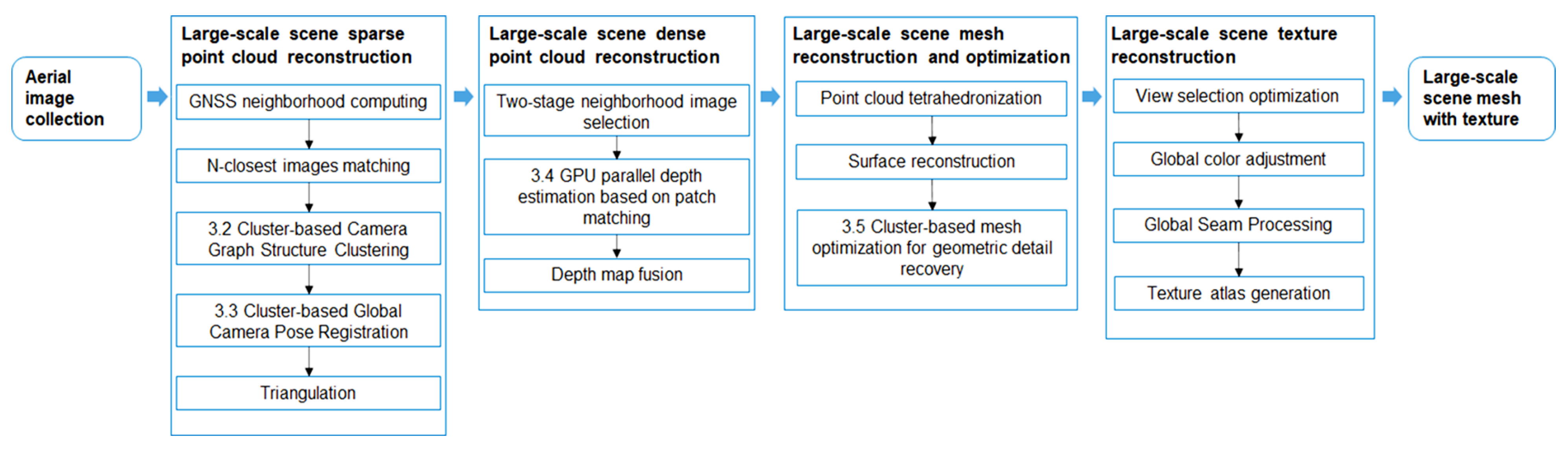
- We propose a cluster-based method for clustering the camera graph algorithm. A divide-and-conquer framework is used to precisely partition the camera graph into several subsets. The algorithm ensures weak correlations between subsets and strong correlations within subsets, which allows the subsets to perform in parallel local camera pose-estimation tasks on cluster nodes.
- We propose a cluster-based global camera pose-alignment algorithm. Using the overlapping camera positions between each subgraph for global camera pose fusion, we mainly solve the nonlinear optimization problem of rotation and translation in the camera pose to obtain a more accurate global camera pose.
- We propose a GPU parallel fast depth-estimation method based on patch matching. The candidate solutions are measured by an improved normalized correlation score, which makes the parallel estimation of image depth values more efficient.
- We propose a cluster-based mesh optimization for the geometric detail-recovery method, which uses the proposed second-order umbrella operator to enhance the mesh’s uniformity and increase the mesh model’s fidelity.
- Compared with similar open-source libraries and commercial reconstruction software, our system can reconstruct large-scale city-level 3D scenes in a cluster environment with one click and has a faster 3D-reconstruction speed within a certain reconstruction quality.
2. Related Work
2.1. 3D Reconstruction Methods
2.1.1. Structure from Motion
2.1.2. Multi-View Stereo
2.1.3. Mesh Optimization
2.2. 3D Reconstruction Libraries and Software
3. System Design
3.1. Overall Structure
3.2. Cluster-Based Camera Graph Structure Clustering
3.2.1. Normalized Cut Algorithm
3.2.2. Camera Graph Division
3.2.3. Camera Graph Expansion
3.3. Cluster-Based Global Camera Pose Registration
3.3.1. Global Rotation Registration
3.3.2. Global Rotation Registration
3.3.3. Optimization of Camera Poses
3.4. GPU Parallel Depth Estimation Based on Patch Matching
3.4.1. Random Initialization of the Depth Normal Vector
3.4.2. Cost Assessment Based on Patch Matching
3.4.3. GPU Parallel Depth Map Generation and Optimization
3.5. Cluster-Based Mesh Optimization for Geometric Detail Recovery
3.5.1. Mesh Simplification
3.5.2. Mesh Smoothing
3.5.3. Mesh-Detail Recovery
4. System Evaluation and Analysis
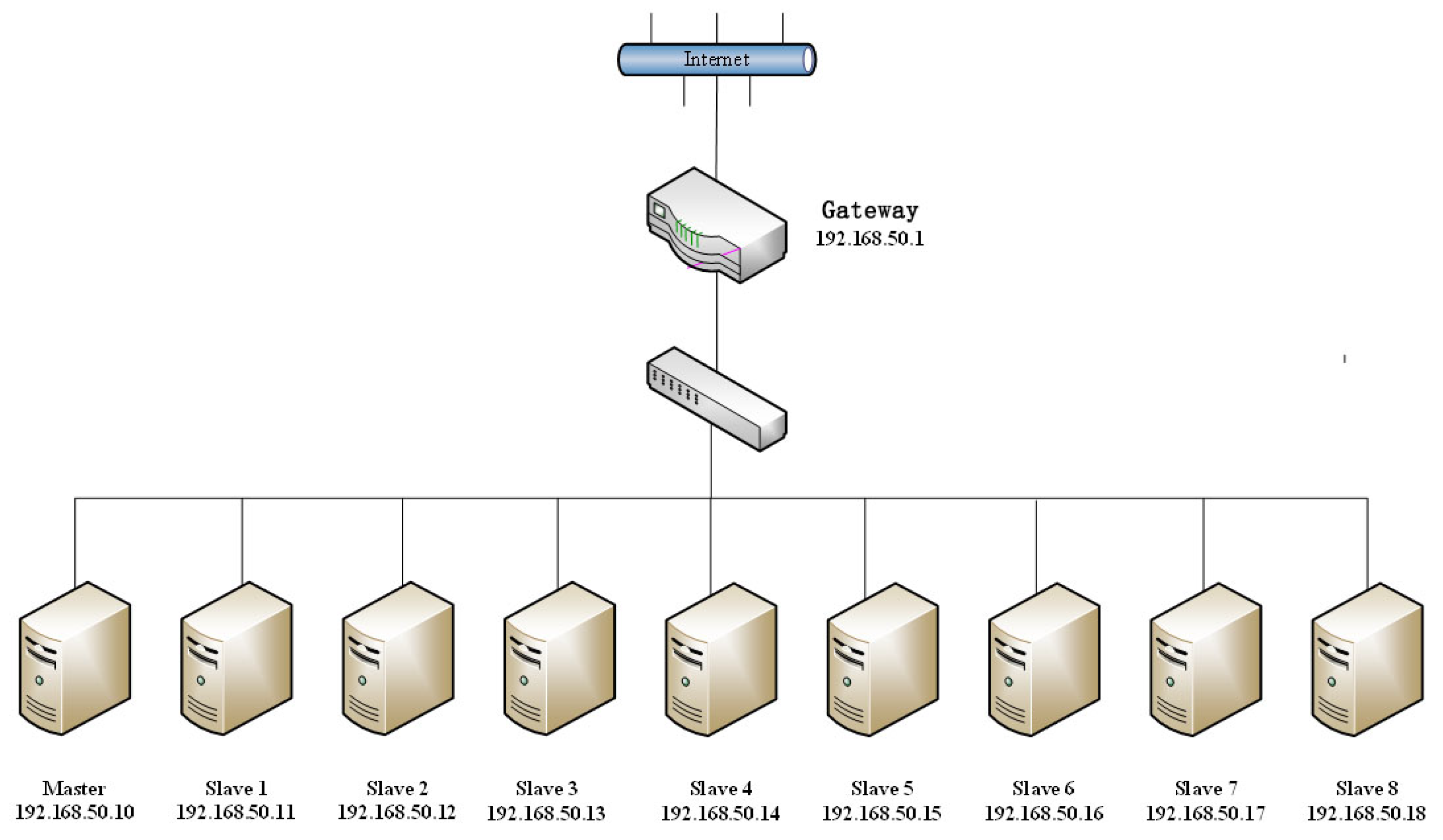
4.1. System Configuration
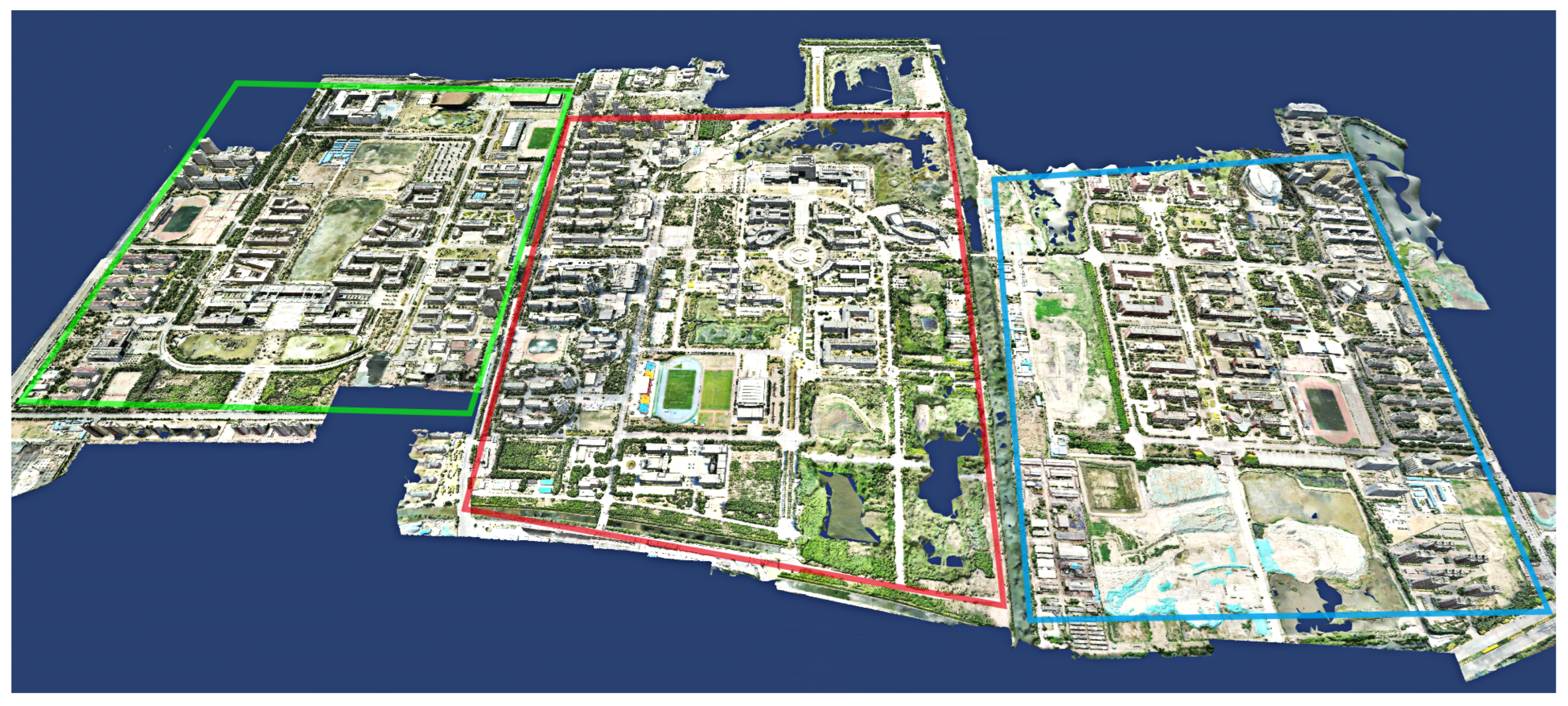
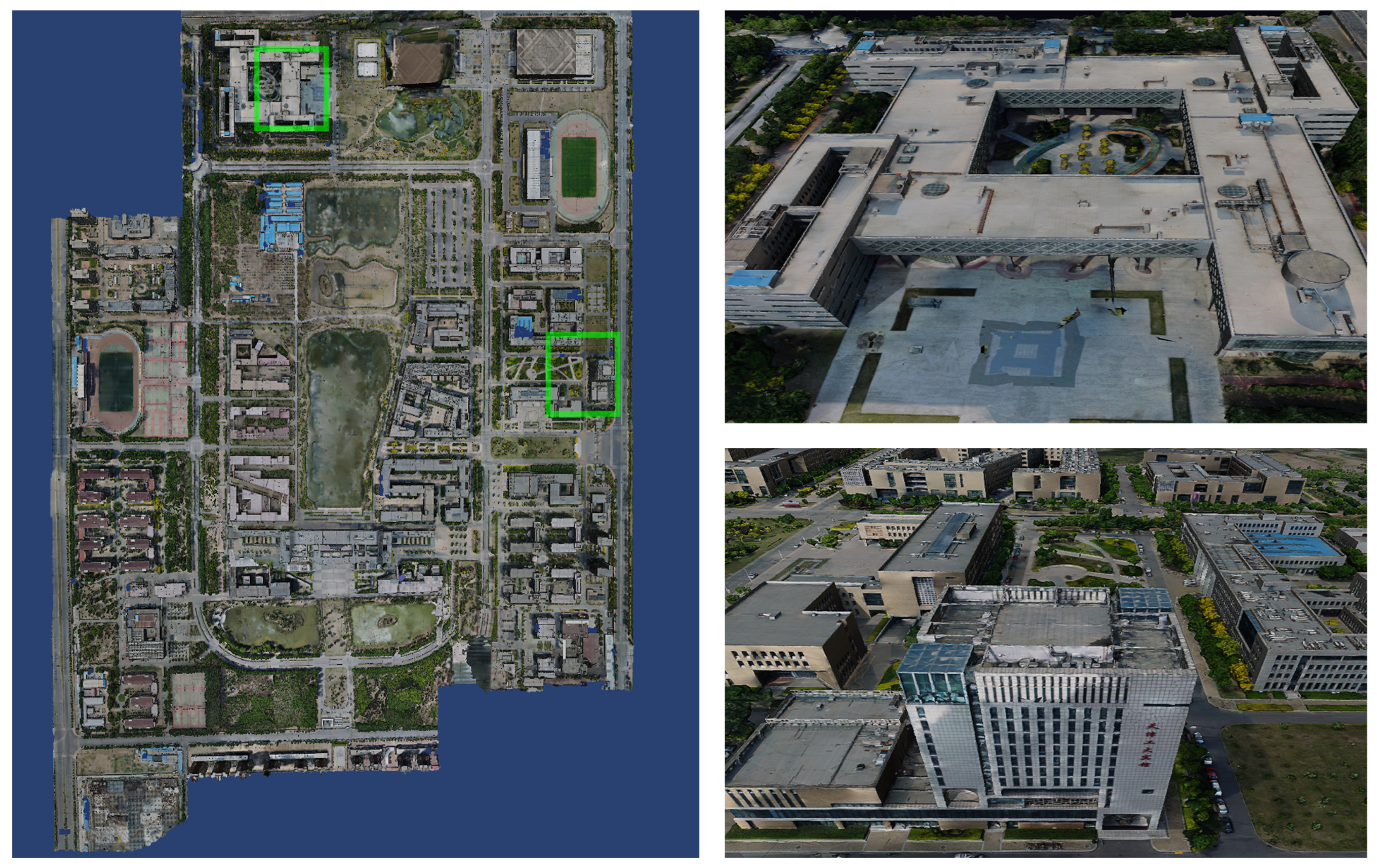
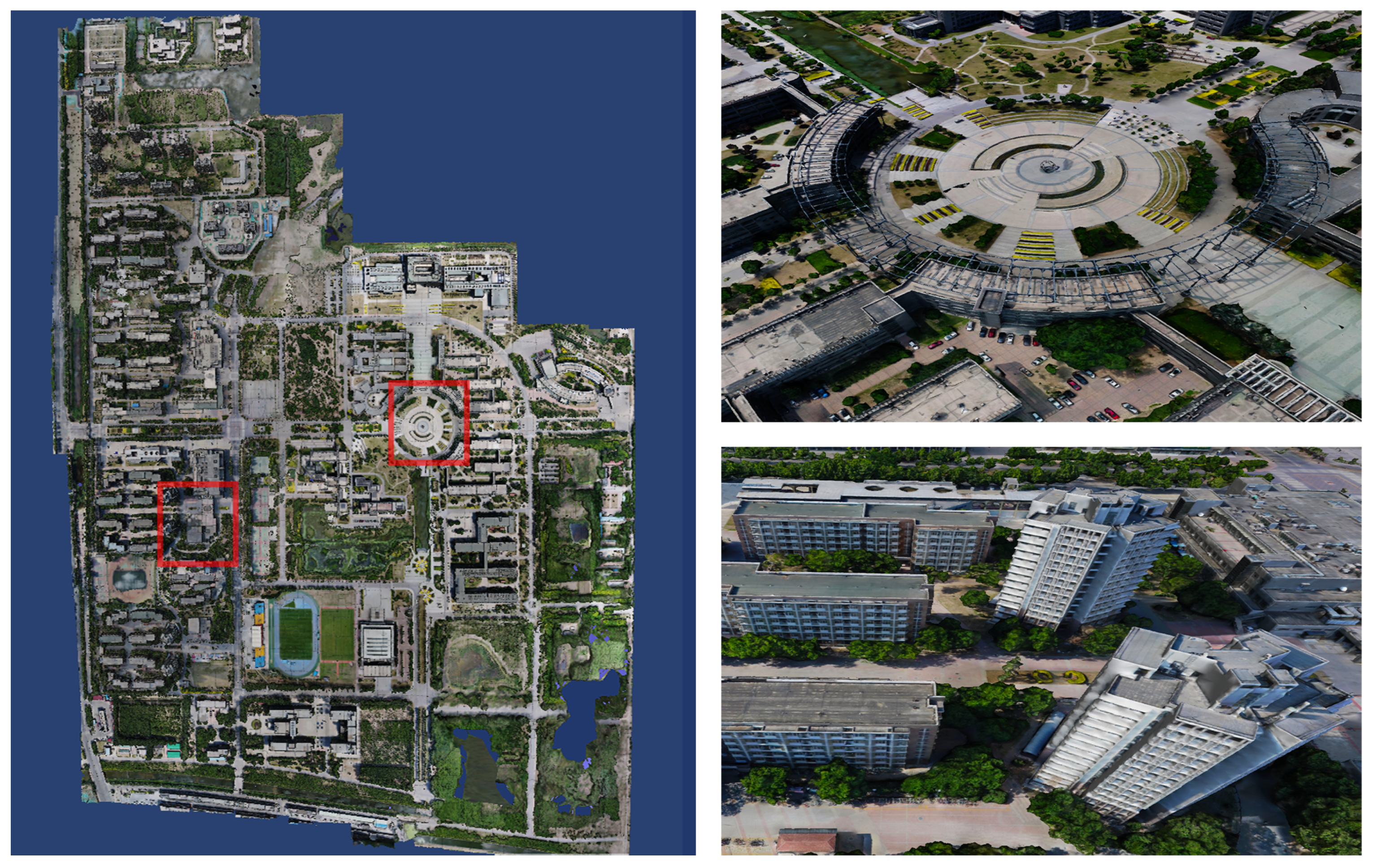
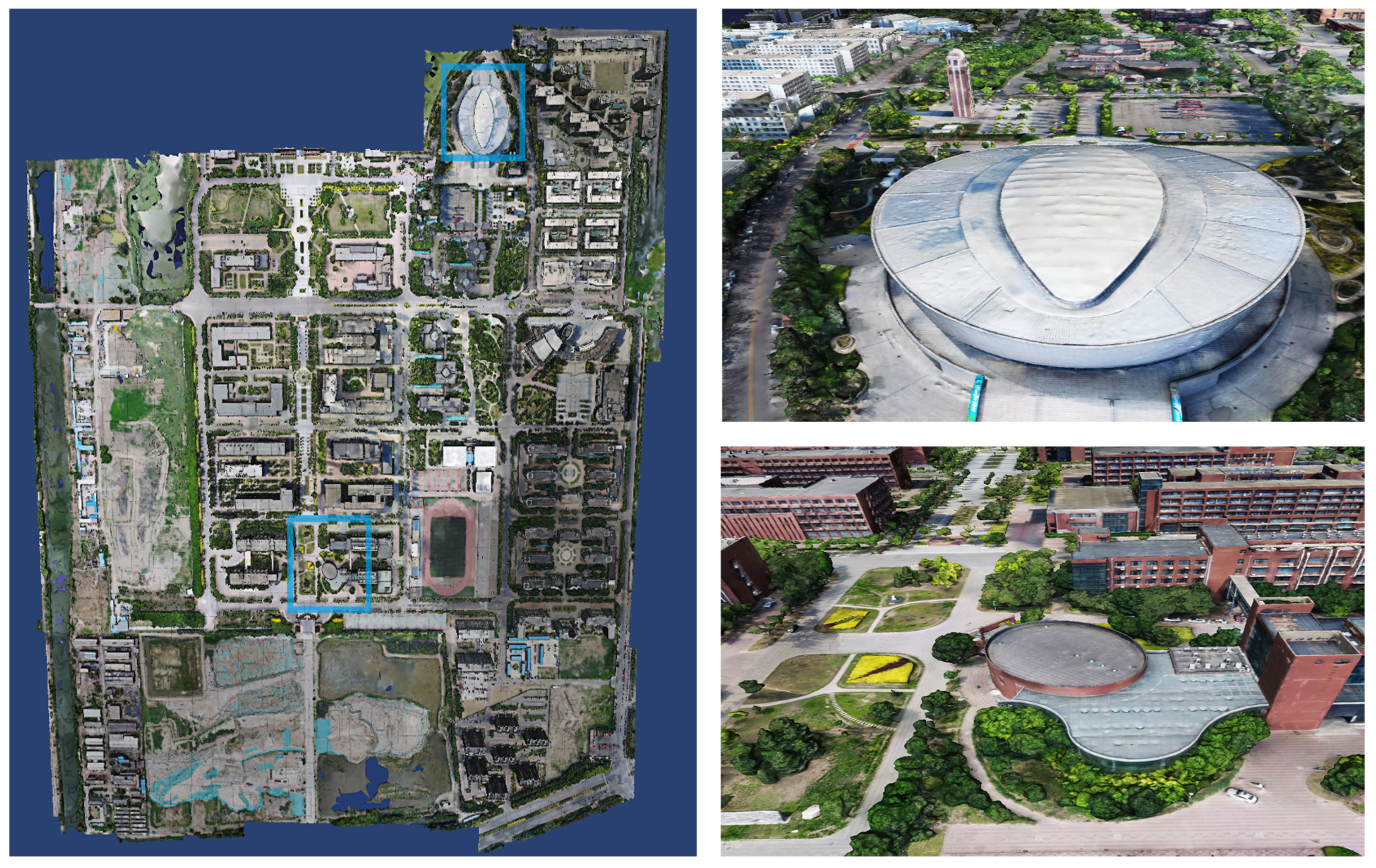
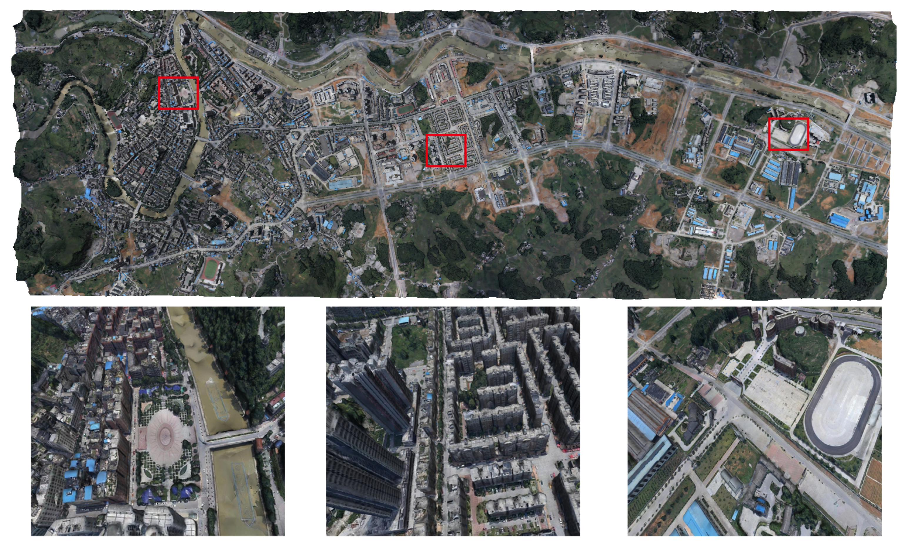
4.2. System Reconstruction Results
4.3. System Comparison
5. System Usage Information
5.1. Simple Mode
5.2. Expert Mode
6. Conclusions
Author Contributions
Funding
Institutional Review Board Statement
Informed Consent Statement
Data Availability Statement
Acknowledgments
Conflicts of Interest
References
- Schonberger, J.L.; Frahm, J.M. Structure-from-motion revisited. In Proceedings of the IEEE Conference on Computer Vision and Pattern Recognition, Las Vegas, NV, USA, 27–30 June 2016; pp. 4104–4113. [Google Scholar]
- Özyeşil, O.; Voroninski, V.; Basri, R.; Singer, A. A survey of structure from motion. Acta Numer. 2017, 26, 305–364. [Google Scholar] [CrossRef]
- Iglhaut, J.; Cabo, C.; Puliti, S.; Piermattei, L.; O’Connor, J.; Rosette, J. Structure from motion photogrammetry in forestry: A review. Curr. For. Rep. 2019, 5, 155–168. [Google Scholar] [CrossRef]
- Agarwal, S.; Furukawa, Y.; Snavely, N.; Simon, I.; Curless, B.; Seitz, S.M.; Szeliski, R. Building rome in a day. Commun. ACM 2011, 54, 105–112. [Google Scholar] [CrossRef]
- Frahm, J.M.; Fite-Georgel, P.; Gallup, D.; Johnson, T.; Raguram, R.; Wu, C.; Jen, Y.H.; Dunn, E.; Clipp, B.; Lazebnik, S.; et al. Building rome on a cloudless day. In Proceedings of the European Conference on Computer Vision, Hersonissos, Crete, Greece, 5–11 September 2010; pp. 368–381. [Google Scholar]
- Jiang, N.; Tan, P.; Cheong, L.F. Seeing double without confusion: Structure-from-motion in highly ambiguous scenes. In Proceedings of the 2012 IEEE Conference on Computer Vision and Pattern Recognition, Providence, Rhode Island, 16–21 June 2012; pp. 1458–1465. [Google Scholar]
- Wu, C. Towards linear-time incremental structure from motion. In Proceedings of the 2013 International Conference on 3D Vision-3DV 2013, Seattle, WA, USA, 29–30 June 2013; pp. 127–134. [Google Scholar]
- Ni, K.; Steedly, D.; Dellaert, F. Out-of-core bundle adjustment for large-scale 3d reconstruction. In Proceedings of the 2007 IEEE 11th International Conference on Computer Vision, Rio De Janeiro, Brazil, 14–21 October 2007; pp. 1–8. [Google Scholar]
- Triggs, B.; McLauchlan, P.F.; Hartley, R.I.; Fitzgibbon, A.W. Bundle adjustment—A modern synthesis. In Proceedings of the International Workshop on Vision Algorithms. Springer, Corfu, Greece, 21–22 September 1999; pp. 298–372. [Google Scholar]
- Agarwal, S.; Snavely, N.; Seitz, S.M.; Szeliski, R. Bundle adjustment in the large. In Proceedings of the European Conference on Computer Vision, Hersonissos, Crete, Greece, 5–11 September 2010; pp. 29–42. [Google Scholar]
- Kneip, L.; Scaramuzza, D.; Siegwart, R. A novel parametrization of the perspective-three-point problem for a direct computation of absolute camera position and orientation. In Proceedings of the CVPR 2011, Colorado Springs, CO, USA, 20–25 June 2011; pp. 2969–2976. [Google Scholar]
- Wu, C.; Agarwal, S.; Curless, B.; Seitz, S.M. Multicore bundle adjustment. In Proceedings of the CVPR 2011, Colorado Springs, CO, USA, 20–25 June 2011; pp. 3057–3064. [Google Scholar]
- Eriksson, A.; Bastian, J.; Chin, T.J.; Isaksson, M. A consensus-based framework for distributed bundle adjustment. In Proceedings of the IEEE Conference on Computer Vision and Pattern Recognition, Las Vegas, NV, USA, 27–30 June 2016; pp. 1754–1762. [Google Scholar]
- Arie-Nachimson, M.; Kovalsky, S.Z.; Kemelmacher-Shlizerman, I.; Singer, A.; Basri, R. Global motion estimation from point matches. In Proceedings of the 2012 Second International Conference on 3D Imaging, Modeling, Processing, Visualization & Transmission, Zurich, Switzerland, 13–15 October 2012; pp. 81–88. [Google Scholar]
- Brand, M.; Antone, M.; Teller, S. Spectral solution of large-scale extrinsic camera calibration as a graph embedding problem. In Proceedings of the European Conference on Computer Vision, Prague, Czech Republic, 11–14 May 2004; pp. 262–273. [Google Scholar]
- Carlone, L.; Tron, R.; Daniilidis, K.; Dellaert, F. Initialization techniques for 3D SLAM: A survey on rotation estimation and its use in pose graph optimization. In Proceedings of the 2015 IEEE iNternational Conference on Robotics and Automation, Seattle, WA, USA, 26–30 May 2015; pp. 4597–4604. [Google Scholar]
- Chatterjee, A.; Govindu, V.M. Efficient and robust large-scale rotation averaging. In Proceedings of the IEEE International Conference on Computer Vision, Sydney, Australia, 1–8 December 2013; pp. 521–528. [Google Scholar]
- Cui, Z.; Tan, P. Global structure-from-motion by similarity averaging. In Proceedings of the IEEE International Conference on Computer Vision, Santiago, Chile, 7–13 December 2015; pp. 864–872. [Google Scholar]
- Cui, Z.; Jiang, N.; Tang, C.; Tan, P. Linear global translation estimation with feature tracks. arXiv 2015, arXiv:1503.01832. [Google Scholar]
- Govindu, V.M. Combining two-view constraints for motion estimation. In Proceedings of the 2001 IEEE Computer Society Conference on Computer Vision and Pattern Recognition (CVPR 2001), Kauai, HI, USA, 8–14 December 2001; Volume 2, p. II. [Google Scholar]
- Govindu, V.M. Lie-algebraic averaging for globally consistent motion estimation. In Proceedings of the 2004 IEEE Computer Society Conference on Computer Vision and Pattern Recognition (CVPR 2004), Washington, DC, USA, 27 June–2 July 2004; Volume 1, p. I. [Google Scholar]
- Ozyesil, O.; Singer, A. Robust camera location estimation by convex programming. In Proceedings of the IEEE Conference on Computer Vision and Pattern Recognition, Boston, MA, USA, 7–12 June 2015; pp. 2674–2683. [Google Scholar]
- Hartley, R.; Trumpf, J.; Dai, Y.; Li, H. Rotation averaging. Int. J. Comput. Vis. 2013, 103, 267–305. [Google Scholar] [CrossRef]
- Sweeney, C.; Fragoso, V.; Höllerer, T.; Turk, M. Large scale sfm with the distributed camera model. In Proceedings of the 2016 Fourth International Conference on 3D Vision, Stanford, CA, USA, 25–28 October 2016; pp. 230–238. [Google Scholar]
- Crandall, D.; Owens, A.; Snavely, N.; Huttenlocher, D. Discrete-continuous optimization for large-scale structure from motion. In Proceedings of the CVPR 2011, Colorado Springs, CO, USA, 20–25 June 2011; pp. 3001–3008. [Google Scholar]
- Cui, H.; Shen, S.; Gao, W.; Hu, Z. Efficient large-scale structure from motion by fusing auxiliary imaging information. IEEE Trans. Image Process. 2015, 24, 3561–3573. [Google Scholar]
- Sweeney, C.; Sattler, T.; Hollerer, T.; Turk, M.; Pollefeys, M. Optimizing the viewing graph for structure-from-motion. In Proceedings of the IEEE international Conference on Computer Vision, Santiago, Chile, 7–13 December 2015; pp. 801–809. [Google Scholar]
- Cui, H.; Gao, X.; Shen, S.; Hu, Z. HSfM: Hybrid structure-from-motion. In Proceedings of the IEEE Conference on Computer Vision and Pattern Recognition, Honolulu, HI, USA, 21–26 July 2017; pp. 1212–1221. [Google Scholar]
- Zhu, S.; Shen, T.; Zhou, L.; Zhang, R.; Wang, J.; Fang, T.; Quan, L. Parallel structure from motion from local increment to global averaging. arXiv 2017, arXiv:1702.08601. [Google Scholar]
- Seo, Y.; Hartley, R. A fast method to minimize error norm for geometric vision problems. In Proceedings of the 2007 IEEE 11th International Conference on Computer Vision, Rio De Janeiro, Brazil, 14–21 October 2007; pp. 1–8. [Google Scholar]
- Zhu, S.; Zhang, R.; Zhou, L.; Shen, T.; Fang, T.; Tan, P.; Quan, L. Very large-scale global sfm by distributed motion averaging. In Proceedings of the IEEE Conference on Computer Vision and Pattern Recognition, Salt Lake City, UT, USA, 18–23 June 2018; pp. 4568–4577. [Google Scholar]
- Furukawa, Y.; Hernández, C. Multi-view stereo: A tutorial. Found. Trends Comput. Graph. Vis. 2015, 9, 1–148. [Google Scholar] [CrossRef]
- Seitz, S.M.; Curless, B.; Diebel, J.; Scharstein, D.; Szeliski, R. A comparison and evaluation of multi-view stereo reconstruction algorithms. In Proceedings of the 2006 IEEE Computer Society Conference on Computer Vision and Pattern Recognition (CVPR 2006), New York, NY, USA, 17–22 June 2006; Volume 1, pp. 519–528. [Google Scholar]
- Goesele, M.; Curless, B.; Seitz, S.M. Multi-view stereo revisited. In Proceedings of the 2006 IEEE Computer Society Conference on Computer Vision and Pattern Recognition (CVPR 2006), New York, NY, USA, 17–22 June 2006; Volume 2, pp. 2402–2409. [Google Scholar]
- Kar, A.; Häne, C.; Malik, J. Learning a multi-view stereo machine. Adv. Neural Inf. Process. Syst. 2017, 30, 1–12. [Google Scholar]
- Vogiatzis, G.; Hernández, C. Video-based, real-time multi-view stereo. Image Vis. Comput. 2011, 29, 434–441. [Google Scholar] [CrossRef]
- Bailer, C.; Finckh, M.; Lensch, H. Scale robust multi view stereo. In Proceedings of the European Conference on Computer Vision, Florence, Italy, 7–13 October 2012; pp. 398–411. [Google Scholar]
- Hiep, V.H.; Keriven, R.; Labatut, P.; Pons, J.P. Towards high-resolution large-scale multi-view stereo. In Proceedings of the 2009 IEEE Conference on Computer Vision and Pattern Recognition, Miami, FL, USA, 20–25 June 2009; pp. 1430–1437. [Google Scholar]
- Habbecke, M.; Kobbelt, L. A surface-growing approach to multi-view stereo reconstruction. In Proceedings of the 2007 IEEE Conference on Computer Vision and Pattern Recognition, Minneapolis, MN, USA, 18–24 June 2007; pp. 1–8. [Google Scholar]
- Goesele, M.; Snavely, N.; Curless, B.; Hoppe, H.; Seitz, S.M. Multi-view stereo for community photo collections. In Proceedings of the 2007 IEEE 11th International Conference on Computer Vision, Rio De Janeiro, Brazil, 14–21 October 2007; pp. 1–8. [Google Scholar]
- Furukawa, Y.; Ponce, J. Accurate, dense, and robust multiview stereopsis. IEEE Trans. Pattern Anal. Mach. Intell. 2009, 32, 1362–1376. [Google Scholar] [CrossRef] [PubMed]
- Seitz, S.M.; Dyer, C.R. Photorealistic scene reconstruction by voxel coloring. Int. J. Comput. Vis. 1999, 35, 151–173. [Google Scholar] [CrossRef]
- Vogiatzis, G.; Torr, P.H.; Cipolla, R. Multi-view stereo via volumetric graph-cuts. In Proceedings of the 2005 IEEE Computer Society Conference on Computer Vision and Pattern Recognition (CVPR 2005), San Diego, CA, USA, 20–26 June 2005; Volume 2, pp. 391–398. [Google Scholar]
- Sinha, S.N.; Mordohai, P.; Pollefeys, M. Multi-view stereo via graph cuts on the dual of an adaptive tetrahedral mesh. In Proceedings of the 2007 IEEE 11th International Conference on Computer Vision, Rio De Janeiro, Brazil, 14–21 October 2007; pp. 1–8. [Google Scholar]
- Li, J.; Li, E.; Chen, Y.; Xu, L.; Zhang, Y. Bundled depth-map merging for multi-view stereo. In Proceedings of the 2010 IEEE Computer Society Conference on Computer Vision and Pattern Recognition, San Francisco, CA, USA, 13–18 June 2010; pp. 2769–2776. [Google Scholar]
- Shen, S. Depth-map merging for multi-view stereo with high resolution images. In Proceedings of the 21st International Conference on Pattern Recognition (ICPR 2012), Tsukuba, Japan, 11–15 November 2012; pp. 788–791. [Google Scholar]
- Shen, S.; Hu, Z. How to select good neighboring images in depth-map merging based 3D modeling. IEEE Trans. Image Process. 2013, 23, 308–318. [Google Scholar] [CrossRef] [PubMed]
- Liu, H.; Tang, X.; Shen, S. Depth-map completion for large indoor scene reconstruction. Pattern Recognit. 2020, 99, 107–112. [Google Scholar] [CrossRef]
- Wei, W.; Wei, G.; ZhanYi, H. Dense 3D scene reconstruction based on semantic constraint and graph cuts. Sci. Sin. Inf. 2014, 44, 774–792. [Google Scholar]
- Schönberger, J.L.; Zheng, E.; Frahm, J.M.; Pollefeys, M. Pixelwise view selection for unstructured multi-view stereo. In Proceedings of the European Conference on Computer Vision, Amsterdam, The Netherlands, 11–14 October 2016; pp. 501–518. [Google Scholar]
- Merrell, P.; Akbarzadeh, A.; Wang, L.; Mordohai, P.; Frahm, J.M.; Yang, R.; Nistér, D.; Pollefeys, M. Real-time visibility-based fusion of depth maps. In Proceedings of the 2007 IEEE 11th International Conference on Computer Vision, Rio De Janeiro, Brazil, 14–21 October 2007; pp. 1–8. [Google Scholar]
- Yao, Y.; Luo, Z.; Li, S.; Fang, T.; Quan, L. Mvsnet: Depth inference for unstructured multi-view stereo. In Proceedings of the European Conference on Computer Vision (ECCV), Munich, Germany, 8–14 September 2018; pp. 767–783. [Google Scholar]
- Yu, Z.; Gao, S. Fast-mvsnet: Sparse-to-dense multi-view stereo with learned propagation and gauss-newton refinement. In Proceedings of the IEEE/CVF Conference on Computer Vision and Pattern Recognition, Seattle, WA, USA, 16–18 June 2020; pp. 1949–1958. [Google Scholar]
- Aanæs, H.; Jensen, R.R.; Vogiatzis, G.; Tola, E.; Dahl, A.B. Large-scale data for multiple-view stereopsis. Int. J. Comput. Vis. 2016, 120, 153–168. [Google Scholar] [CrossRef]
- Khot, T.; Agrawal, S.; Tulsiani, S.; Mertz, C.; Lucey, S.; Hebert, M. Learning unsupervised multi-view stereopsis via robust photometric consistency. arXiv 2019, arXiv:1905.02706. [Google Scholar]
- Dai, Y.; Zhu, Z.; Rao, Z.; Li, B. Mvs2: Deep unsupervised multi-view stereo with multi-view symmetry. In Proceedings of the 2019 International Conference on 3D Vision, Quebec City, Quebec, Canada, 16–19 September 2019; pp. 1–8. [Google Scholar]
- Huang, B.; Yi, H.; Huang, C.; He, Y.; Liu, J.; Liu, X. M3VSNet: Unsupervised multi-metric multi-view stereo network. In Proceedings of the 2021 IEEE International Conference on Image Processing, Anchorage, AK, USA, 19–22 September 2021; pp. 3163–3167. [Google Scholar]
- Xu, H.; Zhou, Z.; Qiao, Y.; Kang, W.; Wu, Q. Self-supervised multi-view stereo via effective co-segmentation and data-augmentation. In Proceedings of the AAAI Conference on Artificial Intelligence, Washington, DC, USA, 7–14 February 2021; Volume 35, pp. 3030–3038. [Google Scholar]
- Garland, M.; Heckbert, P.S. Simplifying surfaces with color and texture using quadric error metrics. In Proceedings of the Proceedings Visualization’98 (Cat. No. 98CB36276), Triangle Park, NC, USA, 18–23 October 1998; pp. 263–269. [Google Scholar]
- Hoppe, H. New quadric metric for simplifying meshes with appearance attributes. In Proceedings of the Proceedings Visualization’99 (Cat. No. 99CB37067), Vienna, Austria, 26–28 May 1999; pp. 59–510. [Google Scholar]
- Williams, N.; Luebke, D.; Cohen, J.D.; Kelley, M.; Schubert, B. Perceptually guided simplification of lit, textured meshes. In Proceedings of the 2003 Symposium on Interactive 3D Graphics, Monterey, CA, USA, 27–30 April 2003; pp. 113–121. [Google Scholar]
- Lindstrom, P.; Turk, G. Image-driven simplification. ACM Trans. Graph. 2000, 19, 204–241. [Google Scholar] [CrossRef]
- Li, W.; Chen, Y.; Wang, Z.; Zhao, W.; Chen, L. An improved decimation of triangle meshes based on curvature. In Proceedings of the International Conference on Rough Sets and Knowledge Technology, Shanghai, China, 24–26 October 2014; pp. 260–271. [Google Scholar]
- An, G.; Watanabe, T.; Kakimoto, M. Mesh simplification using hybrid saliency. In Proceedings of the 2016 International Conference on Cyberworlds, Chongqing, China, 28–30 September 2016; pp. 231–234. [Google Scholar]
- Jiang, Y.; Nie, W.; Tang, L.; Liu, Y.; Liang, R.; Hao, X. Vertex Mesh Simplification Algorithm Based on Curvature and Distance Metric. In Transactions on Edutainment XII; Springer: Berlin/Heidelberg, Germany, 2016; pp. 152–160. [Google Scholar]
- TaubinÝ, G. Geometric signal processing on polygonal meshes. In Proceedings of the Proceedings of Eurographics, Berlin/Heidelberg, Germany, 26–28 June 2000; pp. 1–13. [Google Scholar]
- Desbrun, M. Processing irregular meshes. In Proceedings of the Proceedings SMI, Shape Modeling International 2002, Banff, AB, Canada, 17–22 May 2002; pp. 157–158. [Google Scholar]
- Fleishman, S.; Cohen-Or, D.; Silva, C.T. Robust moving least-squares fitting with sharp features. ACM Trans. Graph. 2005, 24, 544–552. [Google Scholar] [CrossRef]
- Bajaj, C.L.; Xu, G. Adaptive fairing of surface meshes by geometric diffusion. In Proceedings of the Proceedings Fifth International Conference on Information Visualisation, London, UK, 25–27 July 2001; pp. 731–737. [Google Scholar]
- Hildebrandt, K.; Polthier, K. Anisotropic filtering of non-linear surface features. Comput. Graph. Forum 2004, 23, 391–400. [Google Scholar] [CrossRef]
- Lee, K.W.; Wang, W.P. Feature-preserving mesh denoising via bilateral normal filtering. In Proceedings of the Ninth International Conference on Computer Aided Design and Computer Graphics (CAD-CG’05), Hong Kong, China, 7–10 December 2005; p. 6. [Google Scholar]
- Wu, C. VisualSFM: A Visual Structure from Motion System. 2011. Available online: http://ccwu.me/vsfm/index.html (accessed on 10 January 2023).
- Furukawa, Y. Clustering Views for Multi-View Stereo. 2010. Available online: https://www.di.ens.fr/cmvs/ (accessed on 10 January 2023).
- Fuhrmann, S.; Langguth, F.; Goesele, M. Mve-a multi-view reconstruction environment. In Proceedings of the GCH, Darmstadt, Germany, 6–8 October 2014; pp. 11–18. [Google Scholar]
- Waechter, M.; Moehrle, N.; Goesele, M. Let there be color! Large-scale texturing of 3D reconstructions. In Proceedings of the European Conference on Computer Vision, Zurich, Switzerland, 6–12 September 2014; pp. 836–850. [Google Scholar]
- Moulon, P.; Monasse, P.; Perrot, R.; Marlet, R. Openmvg: Open multiple view geometry. In Proceedings of the International Workshop on Reproducible Research in Pattern Recognition, Cancun, Mexico, 29–31 March 2017; pp. 60–74. [Google Scholar]
- Cernea, D. OpenMVS: Multi-View Stereo Reconstruction Library. 2020. Available online: https://cdcseacave.github.io/openMVS (accessed on 10 January 2023).
- Schönberger, J.L.; Price, T.; Sattler, T.; Frahm, J.M.; Pollefeys, M. A Vote-and-Verify Strategy for Fast Spatial Verification in Image Retrieval. In Proceedings of the Asian Conference on Computer Vision (ACCV 2016), Taipei, Taiwan, 20–24 November 2016; pp. 1–16. [Google Scholar]
- Verhoeven, G. Taking computer vision aloft–archaeological three-dimensional reconstructions from aerial photographs with photoscan. Archaeol. Prospect. 2011, 18, 67–73. [Google Scholar] [CrossRef]
- Shi, J.; Malik, J. Normalized cuts and image segmentation. IEEE Trans. Pattern Anal. Mach. Intell. 2000, 22, 888–905. [Google Scholar]
- Martinec, D.; Pajdla, T. Robust rotation and translation estimation in multiview reconstruction. In Proceedings of the 2007 IEEE Conference on Computer Vision and Pattern Recognition, Rio De Janeiro, Brazil, 14–21 October 2007; pp. 1–8. [Google Scholar]
- Xu, Q.; Tao, W. Multi-scale geometric consistency guided multi-view stereo. In Proceedings of the IEEE/CVF Conference on Computer Vision and Pattern Recognition, Long Beach, CA, USA, 15–20 June 2019; pp. 5483–5492. [Google Scholar]
- Wang, F.; Galliani, S.; Vogel, C.; Speciale, P.; Pollefeys, M. Patchmatchnet: Learned multi-view patchmatch stereo. In Proceedings of the IEEE/CVF Conference on Computer Vision and Pattern Recognition, Nashville, TN, USA, 20–25 June 2021; pp. 14194–14203. [Google Scholar]
- Xu, Q.; Kong, W.; Tao, W.; Pollefeys, M. Multi-Scale Geometric Consistency Guided and Planar Prior Assisted Multi-View Stereo. IEEE Trans. Pattern Anal. Mach. Intell. 2022, 1–18. [Google Scholar] [CrossRef] [PubMed]
- Golias, N.; Dutton, R. Delaunay triangulation and 3D adaptive mesh generation. Finite Elem. Anal. Des. 1997, 25, 331–341. [Google Scholar] [CrossRef]
- Li, Y.; Xie, Y.; Wang, X.; Luo, X.; Qi, Y. A Fast Method for Large-Scale Scene Data Acquisition and 3D Reconstruction. In Proceedings of the 2019 IEEE International Symposium on Mixed and Augmented Reality Adjunct (ISMAR-Adjunct), Beijing, China, 10–18 October 2019; pp. 321–325. [Google Scholar]
- Liu, J.; Ji, S. A novel recurrent encoder-decoder structure for large-scale multi-view stereo reconstruction from an open aerial dataset. In Proceedings of the IEEE/CVF Conference on Computer Vision and Pattern Recognition, Seattle, WA, USA, 13–19 June 2020; pp. 6050–6059. [Google Scholar]


| Calculation Node Name | CPU | Graphics Card | Memory |
|---|---|---|---|
| Master | Intel(R) Xeon(R) Gold 3160 CPU @2.10 GHz | Titan RTX | 256 GB |
| Slave1~Slave5 | Intel(R) Core(TM) i7-8700K CPU@3.70 GHz | GeForce GTX1080Ti | 32 GB |
| Slave6~Slave8 | Intel(R) Xeon(R) Sliver 4110 CPU @2.10 GHz | Quadro P6000 | 64 GB |
| System Dependency Library | Version Information |
|---|---|
| Ubuntu | 16.04 |
| Eigen | 3.2.10 |
| Ceres solver | 1.10 |
| C++ | 14 |
| OpenCV | 3.4.11 |
| CGAL | 5.0.1 |
| VCGLib | 1.0.1 |
| Boost | 1.76 |
| 3D Reconstruction Time Consumed (h) | |||||
|---|---|---|---|---|---|
| Library/Software | Version | Cluster | Dataset 1: TPU | Dataset 2: TNU | Dataset 3: TJUT |
| OpenMVG [76] + OpenMVS [77] | V2.0, V2.0 | ✘ | 93.33 | 123.50 | 110.75 |
| Colmap [78] + OpenMVS | V3.7, V2.0 | ✔ | 68.25 | 82.58 | 78.83 |
| Pix4Dmapper | V4.3.9 | ✘ | 90.50 | 110.50 | 101.67 |
| ContextCapture | V4.6.10 | ✔ | 52.17 | 64.33 | 59.75 |
| Ours (standard mode) | V1.0.2 | ✔ | 48.50 | 55.75 | 52.83 |
| Ours (fast mode) | V1.0.2 | ✔ | 23.45 | 27.42 | 25.92 |
| 3D Reconstruction Time Consumed (h) | |||
|---|---|---|---|
| Library/Software | Version | Cluster | Dataset: WHU |
| OpenMVG + OpenMVS | V2.0, V2.0 | ✘ | 69.5 |
| Colmap + OpenMVS | V3.7, V2.0 | ✔ | 34.67 |
| Pix4Dmapper | V4.3.9 | ✘ | 64.25 |
| ContextCapture | V4.6.10 | ✔ | 26.75 |
| Ours (standard mode) | V1.0.2 | ✔ | 24.33 |
| Ours (fast mode) | V1.0.2 | ✔ | 10.83 |
| Operation No. | Operating Steps |
|---|---|
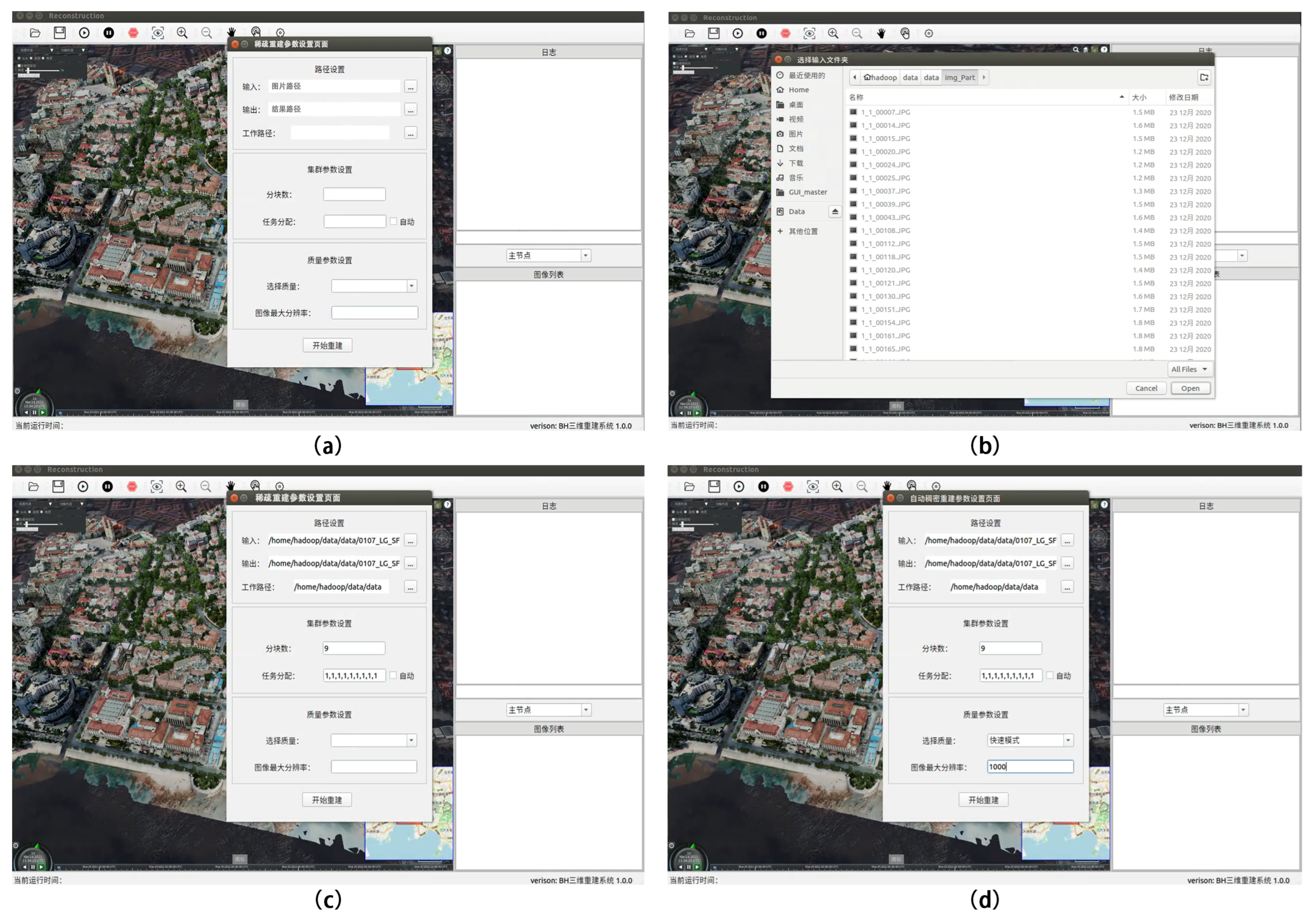
| 1 | On the system home page, click on “Sparse Reconstruction—Sparse Reconstruction Parameter Setting”, as shown in Figure 9a. |
| 2 | As shown in Figure 9b, click the folder selection button on the right side of “Enter image path” to select the path of the input image folder. |
| 3 | Select a storage folder path for the output sparse point-cloud model by clicking the folder selection button on the right side of “Output Path”. |
| 4 | To select the storage path for the intermediate files, click the folder selection button on the right side of the “Work Path”. |
| 5 | Set the number of chunks in the reconstruction area—that is, set the number of compute nodes in the requested cluster. |
| 6 | Figure 9c shows how to set the task allocation ratio of each calculation node or select the check box to allocate tasks evenly by default. |
| 7 | Click the quality selection combo box and select the desired quality of the 3D reconstruction. |
| 8 | Set the image resolution used in the sparse point-cloud reconstruction. |
| 9 | As shown in Figure 9d, click the Start Reconstruction button to begin the fully automated, hands-free process of 3D sparse point-cloud reconstruction. |
| Operation No. | Operating Steps |
|---|---|
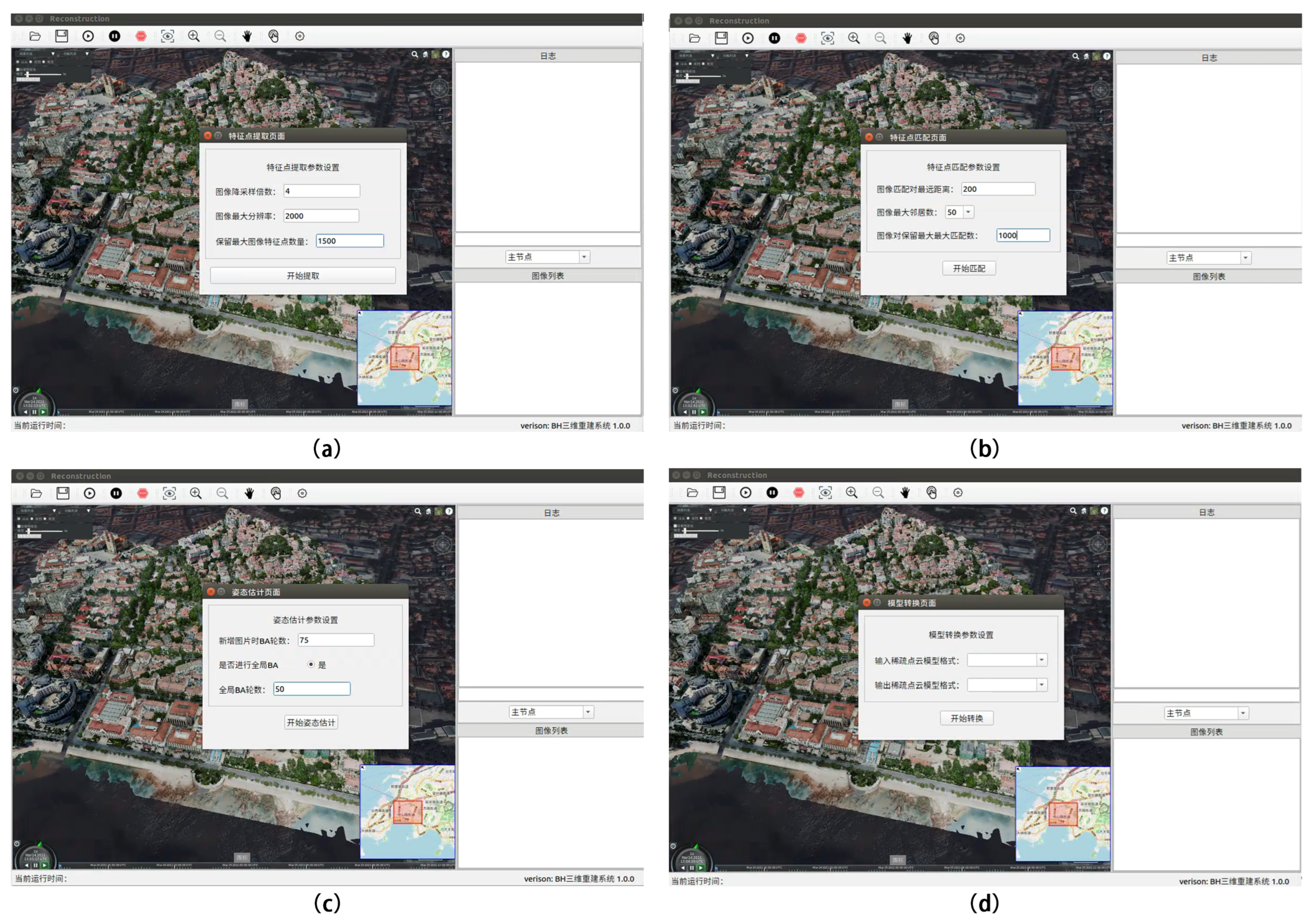
| 1 | On the system home page, the user selects “Sparse Reconstruction-Feature Extraction” in the menu bar, and the “Feature Extraction” dialog box appears. |
| 2 | As shown in Figure 10a, set the downsampling multiplier, the maximum resolution, and the maximum number of retained image features based on the requirements of the user. |
| 3 | The user selects “Sparse Reconstruction-Feature Matching” in the menu bar of the system home page, and the “Feature Matching” dialog box pops up. |
| 4 | Depending upon the user requirements and the actual situation in the scene, determine the farthest distance of image-matching pairs, the maximum number of neighbors for each image (the number of pairs to match), and the maximum number of matches between image-matching pairs, as shown in Figure 10b. |
| 5 | Upon selecting “Sparse Reconstruction-BA” from the menu bar of the system home page, the “BA” dialog box appears. |
| 6 | In Figure 10c, the user specifies the number of BA rounds when adding pictures according to the actual requirements, checks the option to perform a global BA, and enters the number of BA rounds. |
| 7 | As shown in Figure 10d, the “Format Conversion” dialog box appears when the user selects “Sparse Reconstruction-Format Conversion” in the menu bar of the system home page. |
| 8 | Case 1: Output model format. The user may only select the output sparse point cloud model format. That is, the default is the model format following the 3D reconstruction of the sparse point cloud. Case 2: Convert model format. The user can convert the existing point cloud model to another point cloud format supported by the system. |
Disclaimer/Publisher’s Note: The statements, opinions and data contained in all publications are solely those of the individual author(s) and contributor(s) and not of MDPI and/or the editor(s). MDPI and/or the editor(s) disclaim responsibility for any injury to people or property resulting from any ideas, methods, instructions or products referred to in the content. |
© 2023 by the authors. Licensee MDPI, Basel, Switzerland. This article is an open access article distributed under the terms and conditions of the Creative Commons Attribution (CC BY) license (https://creativecommons.org/licenses/by/4.0/).
Share and Cite
Li, Y.; Qi, Y.; Wang, C.; Bao, Y. A Cluster-Based 3D Reconstruction System for Large-Scale Scenes. Sensors 2023, 23, 2377. https://doi.org/10.3390/s23052377
Li Y, Qi Y, Wang C, Bao Y. A Cluster-Based 3D Reconstruction System for Large-Scale Scenes. Sensors. 2023; 23(5):2377. https://doi.org/10.3390/s23052377
Chicago/Turabian StyleLi, Yao, Yue Qi, Chen Wang, and Yongtang Bao. 2023. "A Cluster-Based 3D Reconstruction System for Large-Scale Scenes" Sensors 23, no. 5: 2377. https://doi.org/10.3390/s23052377
APA StyleLi, Y., Qi, Y., Wang, C., & Bao, Y. (2023). A Cluster-Based 3D Reconstruction System for Large-Scale Scenes. Sensors, 23(5), 2377. https://doi.org/10.3390/s23052377