


Cross-Domain Transfer of EEG to EEG or ECG Learning for CNN Classification Models
Abstract
:1. Introduction
2. Materials and Methods
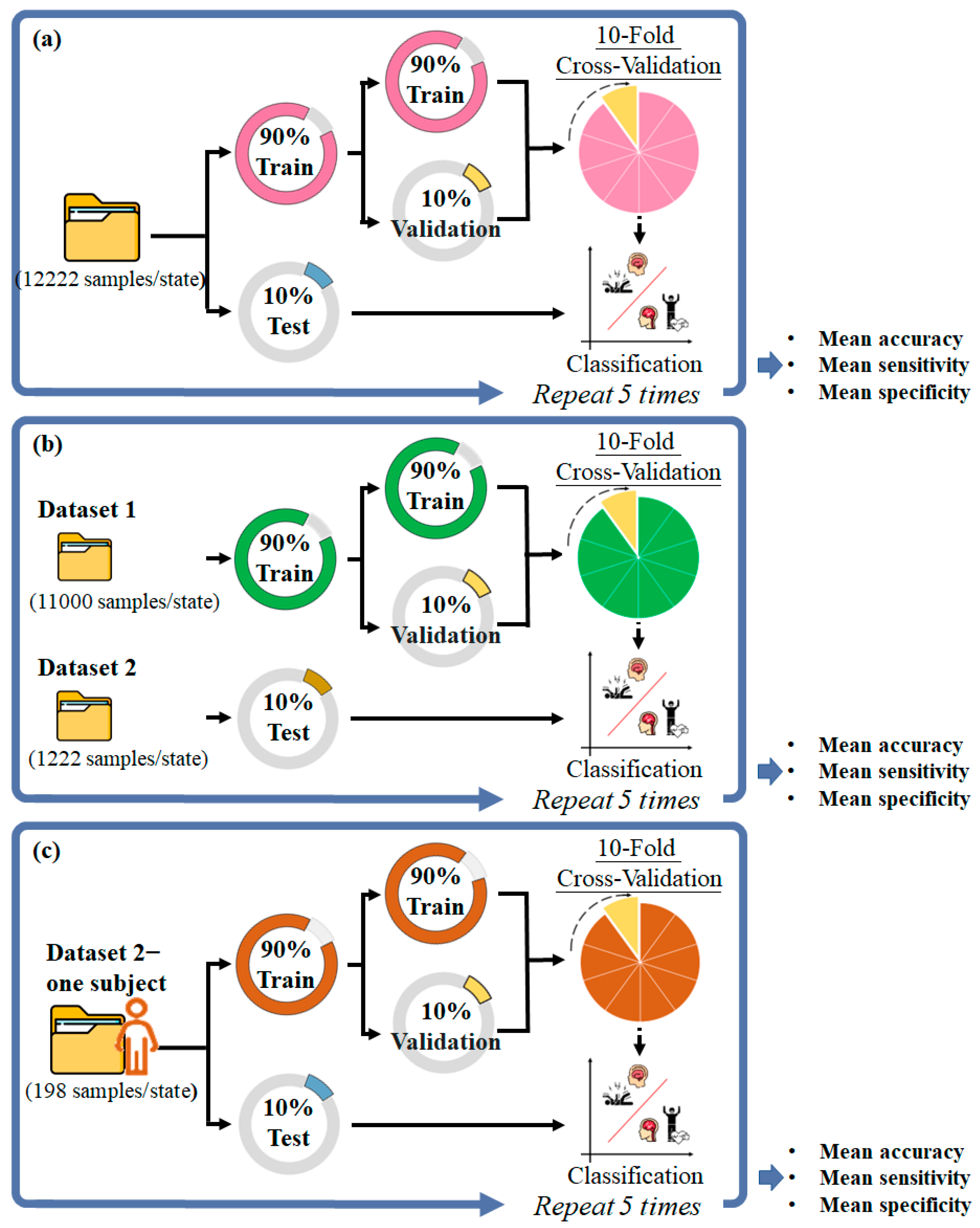
2.1. Experiment 1
2.1.1. Datasets
2.1.2. Data Acquisition
2.1.3. Data Analysis
2.1.4. Classification and Performance Evaluation
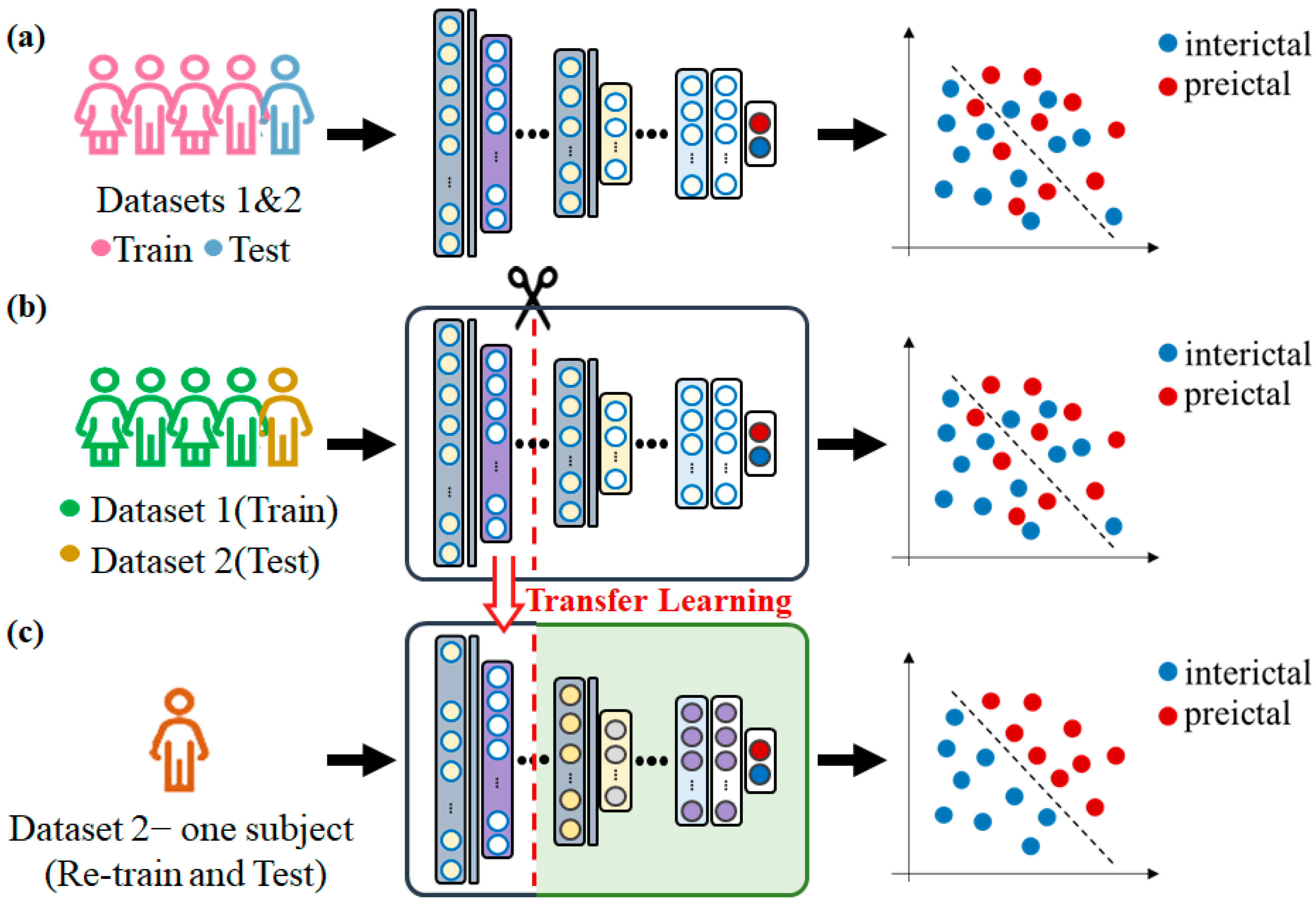
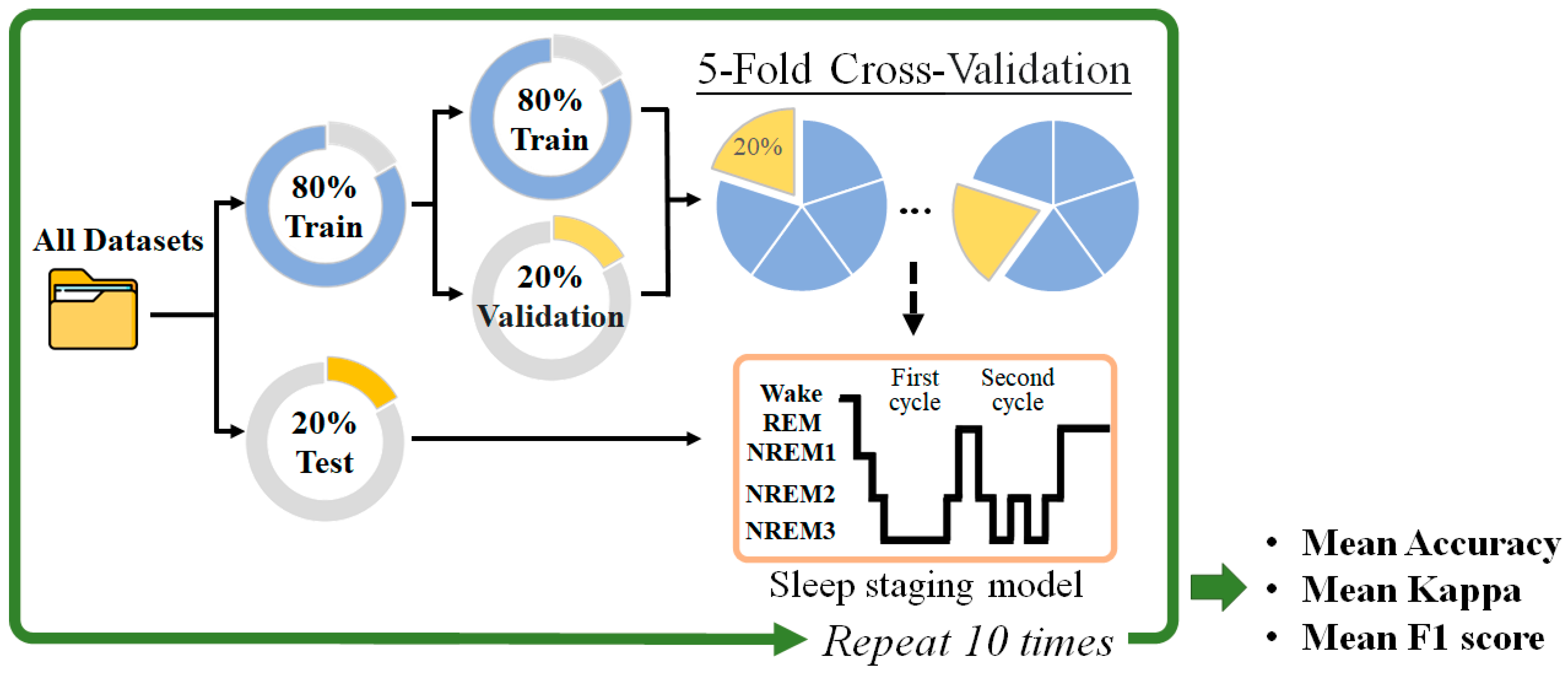
2.2. Experiment 2
2.2.1. Datasets
2.2.2. Data Acquisition
2.2.3. Data Analysis
2.2.4. Classification and Performance Evaluation
3. Results
3.1. Experiment 1
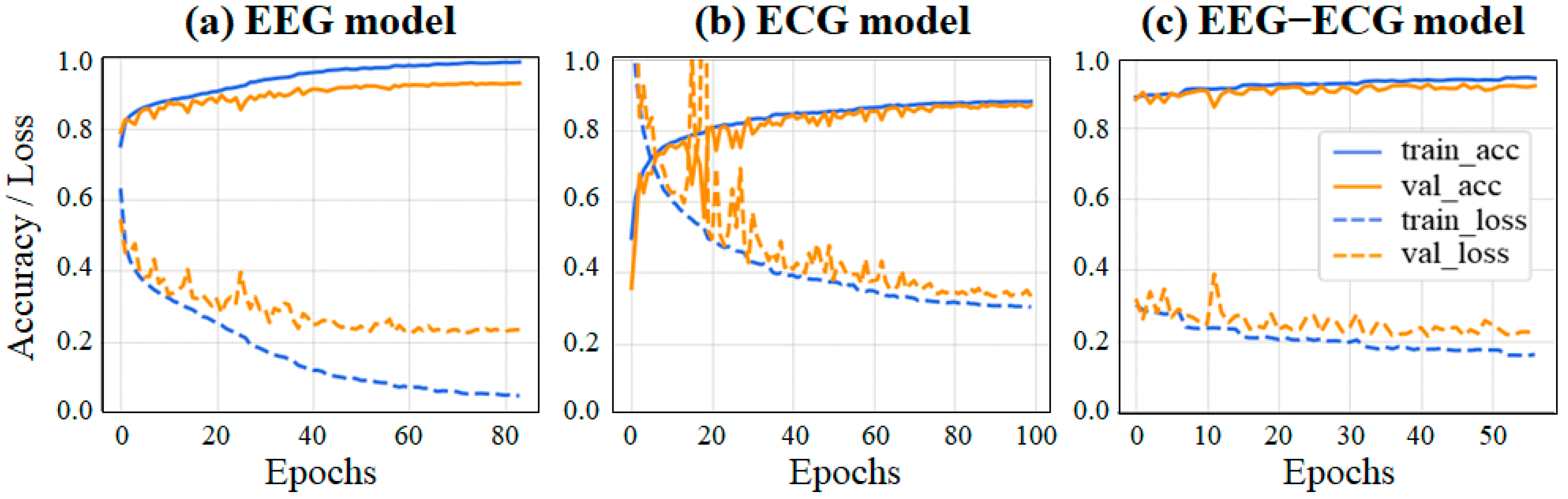
3.2. Experiment 2
4. Discussion
4.1. Experiment 1
4.2. Experiment 2
5. Conclusions
Author Contributions
Funding
Institutional Review Board Statement
Informed Consent Statement
Data Availability Statement
Acknowledgments
Conflicts of Interest
References
- Binnie, C.D.; Prior, P.F. Electroencephalography. J. Neurol. Neurosurg. Psychiatry Res. 1994, 57, 1308–1319. [Google Scholar] [CrossRef] [Green Version]
- Oh, S.L.; Hagiwara, Y.; Raghavendra, U.; Yuvaraj, R.; Arunkumar, N.; Murugappan, M.; Acharya, U.R. A deep learning approach for Parkinson’s disease diagnosis from EEG signals. Neural. Comput. Appl. 2018, 32, 10927–10933. [Google Scholar] [CrossRef]
- Rim, B.; Sung, N.J.; Min, S.; Hong, M. Deep learning in physiological signal data: A survey. Sensors 2020, 20, 969. [Google Scholar] [CrossRef] [PubMed] [Green Version]
- Han, C.; Peng, F.; Chen, C.; Li, W.; Zhang, X.; Wang, X.; Zhou, W. Research progress of epileptic seizure predictions based on electroencephalogram signals. J. Biomed. Eng. 2021, 38, 1193–1202. [Google Scholar] [PubMed]
- Yang, C.Y.; Huang, Y.Z. Parkinson’s Disease Classification Using machine learning approaches and resting-state EEG. J. Med. Biol. Eng. 2022, 42, 263–270. [Google Scholar] [CrossRef]
- Shoeibi, A.; Sadeghi, D.; Moridian, P.; Ghassemi, N.; Heras, J.; Alizadehsani, R.; Khadem, A.; Kong, Y.; Nahavandi, S.; Zhang, Y.; et al. Automatic diagnosis of schizophrenia in EEG signals using CNN-LSTM models. Front. Neurosci. 2021, 15, 777977. [Google Scholar] [CrossRef]
- Cimtay, Y.; Ekmekcioglu, E. Investigating the use of pretrained convolutional neural network on cross-subject and cross-dataset EEG emotion recognition. Sensors 2020, 20, 2034. [Google Scholar] [CrossRef] [Green Version]
- Urtnasan, E.; Park, J.U.; Joo, E.Y.; Lee, K.J. Deep convolutional recurrent model for automatic scoring sleep stages based on single-lead ECG signal. Diagnostics 2022, 12, 1235. [Google Scholar] [CrossRef]
- Panigrahi, S.; Nanda, A.; Swarnkar, T. A Survey on Transfer Learning. In Intelligent and Cloud Computing; Springer: Singapore, 2021; pp. 781–789. [Google Scholar]
- Phan, H.; Chén, O.Y.; Koch, P.; Lu, Z.; McLoughlin, I.; Mertins, A.; De Vos, M. Towards more accurate automatic sleep staging via deep transfer learning. IEEE Trans. Biomed. Eng. 2021, 68, 1787–1798. [Google Scholar] [CrossRef]
- Wan, Z.; Yang, R.; Huang, M.; Zeng, N.; Liu, X. A review on transfer learning in EEG signal analysis. Neurocomputing 2021, 421, 1–14. [Google Scholar] [CrossRef]
- Zargar, B.S.; Mollaei, M.R.K.; Ebrahimi, F.; Rasekhi, J. Generalizable epileptic seizures prediction based on deep transfer learning. Cogn. Neurodyn. 2023, 17, 119–131. [Google Scholar] [CrossRef] [PubMed]
- Bird, J.J.; Kobylarz, J.; Faria, D.R.; Ekárt, A.; Ribeiro, E.P. Cross-domain MLP and CNN transfer learning for biological signal processing: EEG and EMG. IEEE Access 2020, 8, 54789–54801. [Google Scholar] [CrossRef]
- Moshe, S.L.; Perucca, E.; Ryvlin, P.; Tomson, T. Epilepsy: New advances. Lancet 2015, 385, 884–898. [Google Scholar] [CrossRef] [PubMed]
- Lun, X.; Yu, Z.; Chen, T.; Wang, F.; Hou, Y. A Simplified CNN Classification Method for MI-EEG via the Electrode Pairs Signals. Front. Hum. Neurosci. 2020, 14, 338. [Google Scholar] [CrossRef]
- Goldberger, A.L.; Amaral, L.A.; Glass, L.; Hausdorff, J.M.; Ivanov, P.C.; Mark, R.G.; Mietus, J.E.; Moody, G.B.; Peng, C.K.; Stanley, H.E. PhysioBank, PhysioToolkit, and PhysioNet: Components of a new research resource for complex physiologic signals. Circulation 2000, 101, 215–220. [Google Scholar] [CrossRef] [Green Version]
- Detti, P.; Vatti, G.; Zabalo, M.D.L. EEG Synchronization Analysis for seizure prediction: A study on data of noninvasive recordings. Processes 2020, 8, 846. [Google Scholar] [CrossRef]
- Billeci, L.; Marino, D.; Insana, L.; Vatti, G.; Varanini, M. Patient-specific seizure prediction based on heart rate variability and recurrence quantification analysis. PLoS ONE 2020, 13, e0204339. [Google Scholar] [CrossRef] [Green Version]
- Skrandies, W. Data reduction of multichannel fields: Global field power and principal component analysis. Brain Topogr. 1989, 2, 73–80. [Google Scholar] [CrossRef]
- Wang, X.; Wang, X.; Liu, W.; Chang, Z.; Kärkkäinen, T.; Cong, F. One dimensional convolutional neural networks for seizure onset detection using long-term scalp and intracranial EEG. Neurocomputing 2021, 459, 212–222. [Google Scholar] [CrossRef]
- Kemp, B.; Zwinderman, A.H.; Tuk, B.; Kamphuisen, H.A.; Oberyé, J.J. Analysis of a sleep-dependent neuronal feedback loop: The slow-wave microcontinuity of the EEG. IEEE Trans. Biomed. Eng. 2000, 47, 1185–1194. [Google Scholar] [CrossRef]
- Alvarez-Estevez, D.; Rijsman, R.M. Inter-database validation of a deep learning approach for automatic sleep scoring. PLoS ONE 2021, 16, e0256111. [Google Scholar] [CrossRef]
- Hori, T.; Sugita, Y.; Koga, E.; Shirakawa, S.; Inoue, K.; Uchida, S.; Kuwahara, H.; Kousaka, M.; Kobayashi, T.; Tsuji, Y.; et al. Proposed supplements and amendments to ‘A Manual of Standardized Terminology, Techniques and Scoring System for Sleep Stages of Human Subjects’, the Rechtschaffen & Kales (1968) standard. Psychiatry Clin. 2001, 55, 305–310. [Google Scholar]
- Jadhav, P.; Mukhopadhyay, S. Automated Sleep Stage Scoring Using Time-frequency spectra convolution neural network. IEEE Trans. Instrum. Meas. 2022, 71, 2510309. [Google Scholar] [CrossRef]
- Acharya, U.R.; Oh, S.L.; Hagiwara, Y.; Tan, J.H.; Adeli, H. Deep convolutional neural network for the automated detection and diagnosis of seizure using EEG signals. Comput. Biol. Med. 2018, 100, 270–278. [Google Scholar] [CrossRef]
- Wei, X.; Zhou, L.; Zhang, Z.; Chen, Z.; Zhou, Y. Early prediction of epileptic seizures using a long-term recurrent convolutional network. J. Neurosci. 2019, 327, 108395. [Google Scholar] [CrossRef]
- Wang, Y.; Yang, Y.; Cao, G.; Guo, J.; Wei, P.; Feng, T.; Dai, Y.; Huang, J.; Kang, G.; Zhao, G. SEEG-Net: An explainable and deep learning-based cross-subject pathological activity detection method for drug-resistant epilepsy. Comput. Biol. Med. 2022, 148, 105703. [Google Scholar] [CrossRef]
- Al-Kadi, M.I.; Reaz, M.B.I.; Ali, M.A.M. Evolution of electroencephalogram signal analysis techniques during anesthesia. Sensors 2013, 13, 6605–6635. [Google Scholar] [CrossRef] [Green Version]
- Ardalan, Z.; Subbian, V. Transfer learning approaches for neuroimaging analysis: A scoping review. Front. Artif. Intell. 2022, 5, 780405. [Google Scholar] [CrossRef]
- Dissanayake, T.; Fernando, T.; Denman, S.; Sridharan, S.; Fookes, C. Geometric Deep learning for subject independent epileptic seizure prediction using scalp EEG signals. IEEE J. Biomed. Health Inform. 2022, 26, 527–538. [Google Scholar] [CrossRef]
- Zhao, Y.; Li, C.; Qian, R.; Song, R.; Chen, X. Patient-specific seizure prediction via adder nNetwork and supervised contrastive learning. IEEE Trans. Neural. Syst. Rehabil. Eng. 2022, 30, 1536–1547. [Google Scholar] [CrossRef]
- da Silveira, T.L.; Kozakevicius, A.J.; Rodrigues, C.R. Single-channel EEG sleep stage classification based on a streamlined set of statistical features in wavelet domain. Med. Biol. Eng. Comput. 2017, 5, 343–352. [Google Scholar] [CrossRef]
- Yildirim, O.; Baloglu, U.B.; Acharya, U.R. Deep learning model for automated sleep stages classification using PSG signals. Int. J. Environ. Res. Public Health 2019, 16, 599. [Google Scholar] [CrossRef] [PubMed] [Green Version]
- Ebrahimi, F.; Setarehdan, S.K.; Nazeran, H. Automatic sleep staging by simultaneous analysis of ECG and respiratory signals in long epochs. Biomed. Signal. Process. Control 2015, 1, 69–79. [Google Scholar] [CrossRef]
- Wei, Y.; Qi, X.; Wang, H.; Liu, Z.; Wang, G.; Yan, X. A multi-class automatic sleep staging method based on long short-term memory network using single-lead electrocardiogram signals. IEEE Access 2019, 7, 85959–85970. [Google Scholar] [CrossRef]
- Tang, M.; Zhang, Z.; He, Z.; Li, W.; Mou, X.; Du, L.; Wang, P.; Zhao, Z.; Chen, X.; Li, X.; et al. Deep adaptation network for subject-specific sleep stage classification based on a single-lead ECG. Biomed. Signal. Process. Control 2022, 75, 103548. [Google Scholar] [CrossRef]
- Radha, M.; Fonseca, P.; Moreau, A.; Ross, M.; Cerny, A.; Anderer, P.; Long, X.; Aarts, R.M. A deep transfer learning approach for wearable sleep stage classification with photoplethysmography. NPJ Digit. Med. 2021, 4, 135. [Google Scholar] [CrossRef]
- Li, C.; Qi, Y.; Ding, X.; Zhao, J.; Sang, T.; Lee, M. A deep learning method approach for sleep stage classification with EEG spectrogram. Int. J. Environ. Res. Public Health 2022, 19, 6322. [Google Scholar] [CrossRef]


| Layer | Type | Filter Size | # Filter | Stride | Output |
|---|---|---|---|---|---|
| conv1d_1 | Conv1D | 10 | 32 | 2 | 2556 × 32 |
| batch normalization_1 | Batch Normalization | - | - | - | 2556 × 32 |
| max_pooling1d_1 | MaxPooling1D | 3 | 1 | 1 | 2554 × 32 |
| conv1d_2 | Conv1D | 10 | 64 | 2 | 1273 × 32 |
| batch normalization_2 | Batch Normalization | - | - | - | 1273 × 32 |
| max_pooling1d_2 | MaxPooling1D | 3 | 1 | 1 | 1271 × 32 |
| conv1d_3 | Conv1D | 10 | 64 | 2 | 631 × 64 |
| batch normalization_3 | Batch Normalization | - | - | - | 631 × 64 |
| max_pooling1d_3 | MaxPooling1D | 3 | 1 | 1 | 629 × 64 |
| conv1d_4 | Conv1D | 10 | 128 | 1 | 620 × 128 |
| batch normalization_4 | Batch Normalization | - | - | - | 620 × 128 |
| max_pooling1d_4 | MaxPooling1D | 3 | 1 | 1 | 618 × 128 |
| global_average_pooling1d | GlobalAveragepooling | - | - | - | 128 |
| dense_1 | Dense | - | - | - | 256 |
| dense_2 | Dense | - | - | - | 128 |
| dense_3 | Dense | - | - | - | 2 |
| Block | Layer | Type | Filter Size | # Filter | Stride | Output |
|---|---|---|---|---|---|---|
| Block_1 | conv1d_1 | Conv1D | 5 | 16 | 1 | 2996 × 16 |
| batch normalization_1 | Batch Normalization | - | - | - | 2996 × 16 | |
| conv1d_2 | Conv1D | 5 | 16 | 1 | 2994 × 16 | |
| batch normalization_2 | Batch Normalization | - | - | - | 2994 × 16 | |
| average_pooling1d_1 | AveragePooling1D | 2 | 1 | 2 | 1496 × 16 | |
| Block_2 | conv1d_3 | Conv1D | 5 | 32 | 1 | 1492 × 32 |
| batch normalization_3 | Batch Normalization | - | - | - | 1492 × 32 | |
| conv1d_4 | Conv1D | 5 | 32 | 1 | 1488 × 32 | |
| batch normalization_4 | Batch Normalization | - | - | - | 1488 × 32 | |
| average_pooling1d_2 | AveragePooling1D | 2 | 1 | 2 | 744 × 32 | |
| Block_3 | conv1d_5 | Conv1D | 5 | 32 | 1 | 740 × 32 |
| batch normalization_5 | Batch Normalization | - | - | - | 740 × 32 | |
| global_average_pooling1d | GlobalAveragepooling | - | - | - | 32 | |
| dense_1 | Dense | - | - | - | 32 | |
| dense_2 | Dense | - | - | - | 5 |
| Record-Wise Training | ||||
| Accuracy (%) | Sensitivity (%) | Specificity (%) | Time | |
| preictal 20–10 | 99.37 (±0.14%) | 99.47 (±024%) | 99.27 (±047%) | 2 h 12 min 43 s |
| preictal 30–20 | 98.61 (±0.20%) | 98.21 (±0.12%) | 99.03 (±0.35%) | 2 h 13 min 43 s |
| preictal 40–30 | 99.59 (±0.22%) | 99.77 (±0.13%) | 99.40 (±0.44%) | 2 h 04 min 06 s |
| Subject-WiseTraining | ||||
| Accuracy (%) | Sensitivity (%) | Specificity (%) | Time | |
| preictal 20–10 | 84.25 (±0.20%) | 82.45 (±1.39%) | 82.45 (±1.39%) | 2 h 17 min 07 s |
| preictal 30–20 | 84.46 (±0.20%) | 84.81 (±0.94%) | 84.12 (±1.09%) | 2 h 19 min 11 s |
| preictal 40–30 | 86.17 (±0.84%) | 88.73 (±0.90%) | 83.60 (±2.05%) | 2 h 20 min 03 s |
| NO. | # of Frozen Layers | Preictal 20–10 | Preictal 30–20 | Preictal 40–30 | |||||||||
|---|---|---|---|---|---|---|---|---|---|---|---|---|---|
| Acc (%) | Sen (%) | Spe (%) | Time (s) | Acc (%) | Sen (%) | Spe (%) | Time (s) | Acc (%) | Sen (%) | Spe (%) | Time (s) | ||
| 2 | 3 | 98.0 | 96.1 | 100 | 42 | 100 | 100 | 100 | 39 | 99.5 | 100 | 99.1 | 43 |
| 6 | 100 | 100 | 100 | 40 | 100 | 100 | 100 | 37 | 100 | 100 | 100 | 37 | |
| 9 | 100 | 100 | 100 | 35 | 100 | 100 | 100 | 46 | 100 | 100 | 100 | 35 | |
| 12 | 97.5 | 100 | 94.7 | 104 | 97.0 | 93.3 | 100 | 112 | 100 | 100 | 100 | 107 | |
| 4 | 3 | 100 | 100 | 100 | 42 | 100 | 100 | 100 | 41 | 100 | 100 | 100 | 43 |
| 6 | 100 | 100 | 100 | 37 | 100 | 100 | 100 | 37 | 100 | 100 | 100 | 35 | |
| 9 | 100 | 100 | 100 | 35 | 100 | 100 | 100 | 46 | 100 | 100 | 100 | 33 | |
| 12 | 94.9 | 90.4 | 100 | 107 | 100 | 100 | 100 | 118 | 97.5 | 100 | 95.4 | 109 | |
| 5 | 3 | 100 | 100 | 100 | 39 | 100 | 100 | 100 | 37 | 100 | 100 | 100 | 33 |
| 6 | 100 | 100 | 100 | 34 | 100 | 100 | 100 | 34 | 100 | 100 | 100 | 31 | |
| 9 | 100 | 100 | 100 | 43 | 100 | 100 | 100 | 30 | 100 | 100 | 100 | 28 | |
| 12 | 100 | 100 | 100 | 107 | 100 | 100 | 100 | 109 | 100 | 100 | 100 | 103 | |
| 7 | 3 | 100 | 100 | 100 | 39 | 100 | 100 | 100 | 36 | 100 | 100 | 100 | 42 |
| 6 | 100 | 100 | 100 | 36 | 100 | 100 | 100 | 32 | 100 | 100 | 100 | 35 | |
| 9 | 100 | 100 | 100 | 44 | 100 | 100 | 100 | 33 | 100 | 100 | 100 | 32 | |
| 12 | 100 | 100 | 100 | 109 | 100 | 100 | 100 | 109 | 100 | 100 | 100 | 109 | |
| 8 | 3 | 100 | 100 | 100 | 41 | 100 | 100 | 100 | 56 | 100 | 100 | 100 | 37 |
| 6 | 100 | 100 | 100 | 32 | 100 | 100 | 100 | 33 | 100 | 100 | 100 | 36 | |
| 9 | 100 | 100 | 100 | 28 | 100 | 100 | 100 | 29 | 100 | 100 | 100 | 36 | |
| 12 | 100 | 100 | 100 | 109 | 100 | 100 | 100 | 109 | 99.5 | 100 | 97.7 | 109 | |
| 9 | 3 | 100 | 100 | 100 | 35 | 99.5 | 100 | 99.33 | 37 | 100 | 100 | 100 | 49 |
| 6 | 100 | 100 | 100 | 37 | 100 | 100 | 100 | 35 | 100 | 100 | 100 | 35 | |
| 9 | 100 | 100 | 100 | 33 | 100 | 100 | 100 | 34 | 100 | 100 | 100 | 31 | |
| 12 | 100 | 100 | 100 | 108 | 97.5 | 100 | 96.66 | 100 | 100 | 100 | 100 | 109 | |
| 10 | 3 | 100 | 100 | 100 | 46 | 100 | 100 | 100 | 44 | 100 | 100 | 100 | 46 |
| 6 | 100 | 100 | 100 | 34 | 100 | 100 | 100 | 40 | 100 | 100 | 100 | 36 | |
| 9 | 100 | 100 | 100 | 33 | 100 | 100 | 100 | 33 | 100 | 100 | 100 | 32 | |
| 12 | 97.5 | 94.7 | 100 | 89 | 100 | 100 | 100 | 109 | 100 | 100 | 100 | 109 | |
| 11 | 3 | 100 | 100 | 100 | 40 | 97.5 | 94.11 | 100 | 41 | 99.5 | 100 | 98.57 | 36 |
| 6 | 100 | 100 | 100 | 31 | 99 | 97.64 | 100 | 38 | 99.5 | 99.23 | 100 | 33 | |
| 9 | 100 | 100 | 100 | 30 | 98.99 | 100 | 98.6 | 33 | 97.5 | 96.15 | 100 | 29 | |
| 12 | 100 | 100 | 100 | 109 | 94.99 | 88.23 | 100 | 109 | 97.5 | 96.1 | 100 | 109 | |
| 13 | 3 | 100 | 100 | 100 | 48 | 98 | 95.7 | 100 | 36 | 100 | 100 | 100 | 34 |
| 6 | 100 | 100 | 100 | 36 | 99.9 | 98.9 | 100 | 28 | 100 | 100 | 100 | 36 | |
| 9 | 100 | 100 | 100 | 30 | 100 | 100 | 100 | 28 | 100 | 100 | 100 | 29 | |
| 12 | 100 | 100 | 100 | 109 | 100 | 100 | 100 | 105 | 100 | 100 | 100 | 106 | |
| Model | Accuracy | Kappa | F1 | Time |
|---|---|---|---|---|
| EEG | 92.67 (±0.45%) | 0.908 (±0.006) | 92.69 (±0.45%) | 1 h 32 min 42 s |
| ECG | 86.13 (±1.49%) | 0.827 (±0.019) | 86.07 (±1.46%) | 1 h 38 min 10 s |
| EEG–ECG (frozen block_1) | 88.64 (±1.00%) | 0.858 (±0.013) | 88.59 (±1.01%) | 47 min 31 s |
| EEG–ECG (frozen block_1&2) | 82.16 (±0.56%) | 0.777 (±0.007) | 82.12 (±0.52%) | 17 min 00 s |
| EEG–ECG (frozen block_1~3) | 63.38 (±0.62%) | 0.542 (±0.008) | 63.19 (±0.60%) | 17 min 05 s |
| Study | Dataset | Input | Model | Training Type | Acc (%) | Sen (%) | Spe (%) |
|---|---|---|---|---|---|---|---|
| Dissanayake et al. [30] | Siena EEG | MFCCs | C-GNN (distance-based) | S-Ind | 96.0 | 96.0 | 96.6 |
| C-GNN (partially learned) | 95.5 | 95.1 | 95.1 | ||||
| Zhao et al. [31] | CHB-MIT | Raw data | 1D-CNN | P-Spc | - | 88.7 | - |
| ResCNN | 89.9 | ||||||
| SCL-AddNets | 93 | ||||||
| This Study | CHB-MIT | Raw data (GFP) | 1D-CNN + transfer learning | P-Spc | 99.73 | 99.79 | 99.65 |
| Siena EEG + Zenodo | Raw data (GFP) | 1D-CNN + transfer learning | P-Spc | 99.9 | 99.9 | 100 |
| Study | Dataset | Input | Model | # CNN Layer | Sleep Stage | Acc (%) | Kappa | F1 (%) |
|---|---|---|---|---|---|---|---|---|
| Li et al. [38] | sleep-edfx | Spectrogram | EEGSNet | 15 | Wake-REM-N1-N2-N3 | 83.02 | 0.770 | 77.26 |
| Jadhav et al. [24] | sleep-edfx | Raw data | 1D-CNN | 6 | Wake-REM-N1-N2-N3 | 83.59 | 0.780 | 77.00 |
| SWT | 2D-CNN | 6 | 85.49 | 0.800 | 78.70 | |||
| STFT | 2D-CNN | 4 | 85.81 | 0.800 | 79.70 | |||
| This Study | sleep-edfx | Raw data | 1D-CNN | 5 | Wake-REM-N1-N2-N3 | 92.67 | 0.908 | 92.69 |
| Study | Dataset | Input | Model | # Class | Sleep Stages | Acc (%) | Kappa | F1 (%) |
|---|---|---|---|---|---|---|---|---|
| Urtnasan et al. [8] | Samsung Medical Center | Raw data | CNN+GRU | 3 | Wake-NREM-REM | 86.40 | - | - |
| 5 | Wake-REM-N1-N2-N3 | 74.20 | - | - | ||||
| Tang et al. [36] | SHHS2 | Raw data | CNN+GRU (Domain adaptation) | 4 | Wake-REM- Light-Deep | 78.70 | 0.749 | - |
| SHHS1 | 74.80 | 0.675 | - | |||||
| MESA | 80.60 | 0.705 | - | |||||
| This Study | HMC sleep center | Raw data | 1D-CNN (ECG) | 5 | Wake-REM-N1-N2-N3 | 86.13 | 0.827 | 86.07 |
| 1D-CNN (EEG-ECG) | 88.64 | 0.858 | 88.59 |
Disclaimer/Publisher’s Note: The statements, opinions and data contained in all publications are solely those of the individual author(s) and contributor(s) and not of MDPI and/or the editor(s). MDPI and/or the editor(s) disclaim responsibility for any injury to people or property resulting from any ideas, methods, instructions or products referred to in the content. |
© 2023 by the authors. Licensee MDPI, Basel, Switzerland. This article is an open access article distributed under the terms and conditions of the Creative Commons Attribution (CC BY) license (https://creativecommons.org/licenses/by/4.0/).
Share and Cite
Yang, C.-Y.; Chen, P.-C.; Huang, W.-C. Cross-Domain Transfer of EEG to EEG or ECG Learning for CNN Classification Models. Sensors 2023, 23, 2458. https://doi.org/10.3390/s23052458
Yang C-Y, Chen P-C, Huang W-C. Cross-Domain Transfer of EEG to EEG or ECG Learning for CNN Classification Models. Sensors. 2023; 23(5):2458. https://doi.org/10.3390/s23052458
Chicago/Turabian StyleYang, Chia-Yen, Pin-Chen Chen, and Wen-Chen Huang. 2023. "Cross-Domain Transfer of EEG to EEG or ECG Learning for CNN Classification Models" Sensors 23, no. 5: 2458. https://doi.org/10.3390/s23052458
APA StyleYang, C.-Y., Chen, P.-C., & Huang, W.-C. (2023). Cross-Domain Transfer of EEG to EEG or ECG Learning for CNN Classification Models. Sensors, 23(5), 2458. https://doi.org/10.3390/s23052458