
Self-Supervised Wavelet-Based Attention Network for Semantic Segmentation of MRI Brain Tumor

 , , , and
Abstract
:1. Introduction
- 1251 patients’ 3D MRI datasets were gathered from the BraTS dataset in the research.
- The Self Supervised Wavelet-based Attention Network (SSW-AN), which splits low-frequency and high-frequency data into four channels, employs the 2D Wavelet transform.
- We use self-supervised attention channels and spatial attention modules (SSAB).
- We give in-depth analysis of the scientific advancements achieved in the field of semantic image segmentation for natural and medical images.
- We discuss the literature on the various medical imaging modalities, including both 2D and volumetric images.
2. Problem Statement
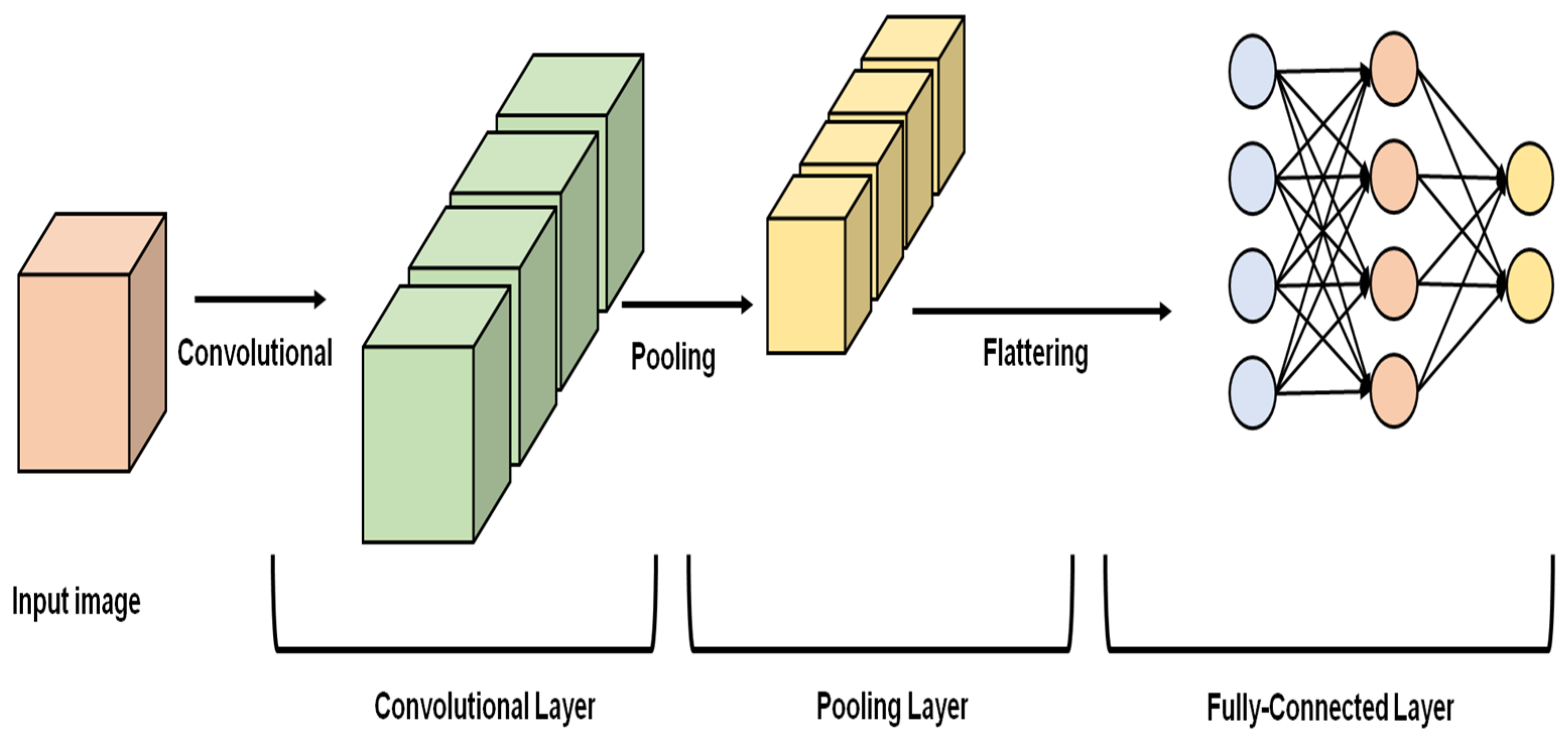
3. Methodology
3.1. Self-Supervised Wavelet-Based Attention Network
3.2. Channel Attention Module
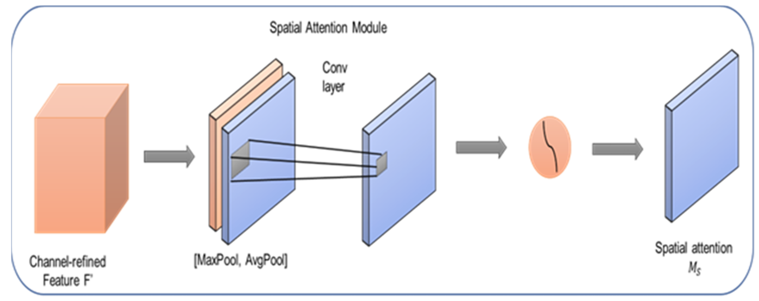
3.3. Spatial Attention Module
4. Loss Function
5. Results and Discussion
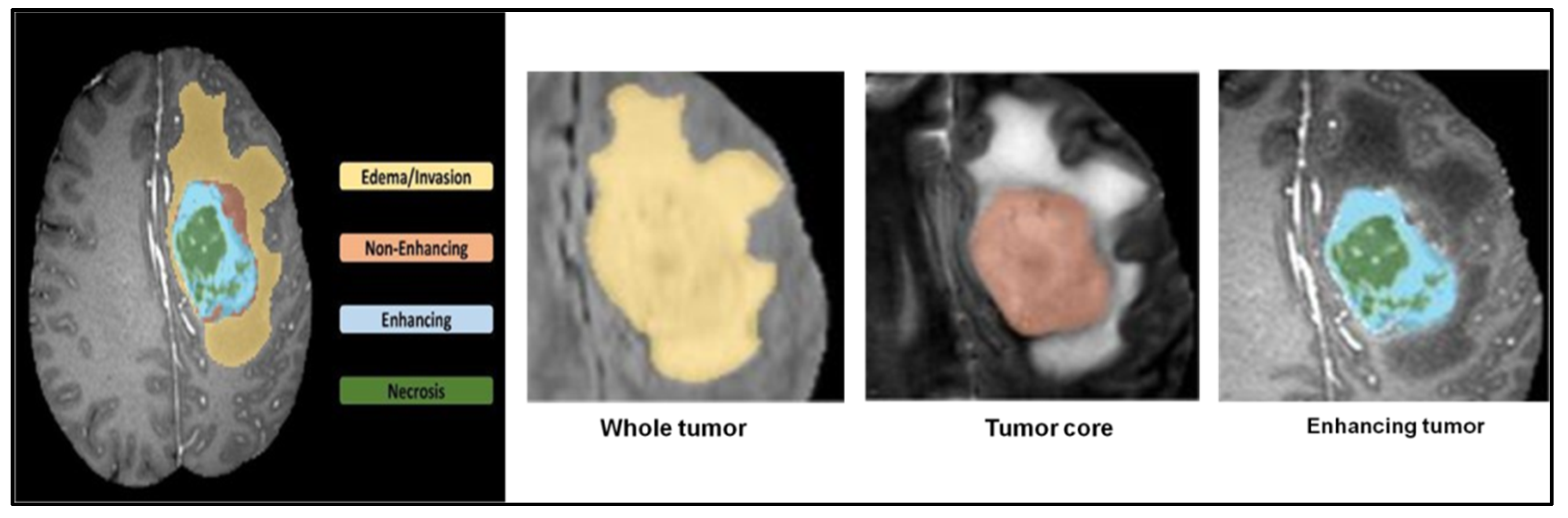
5.1. Dataset
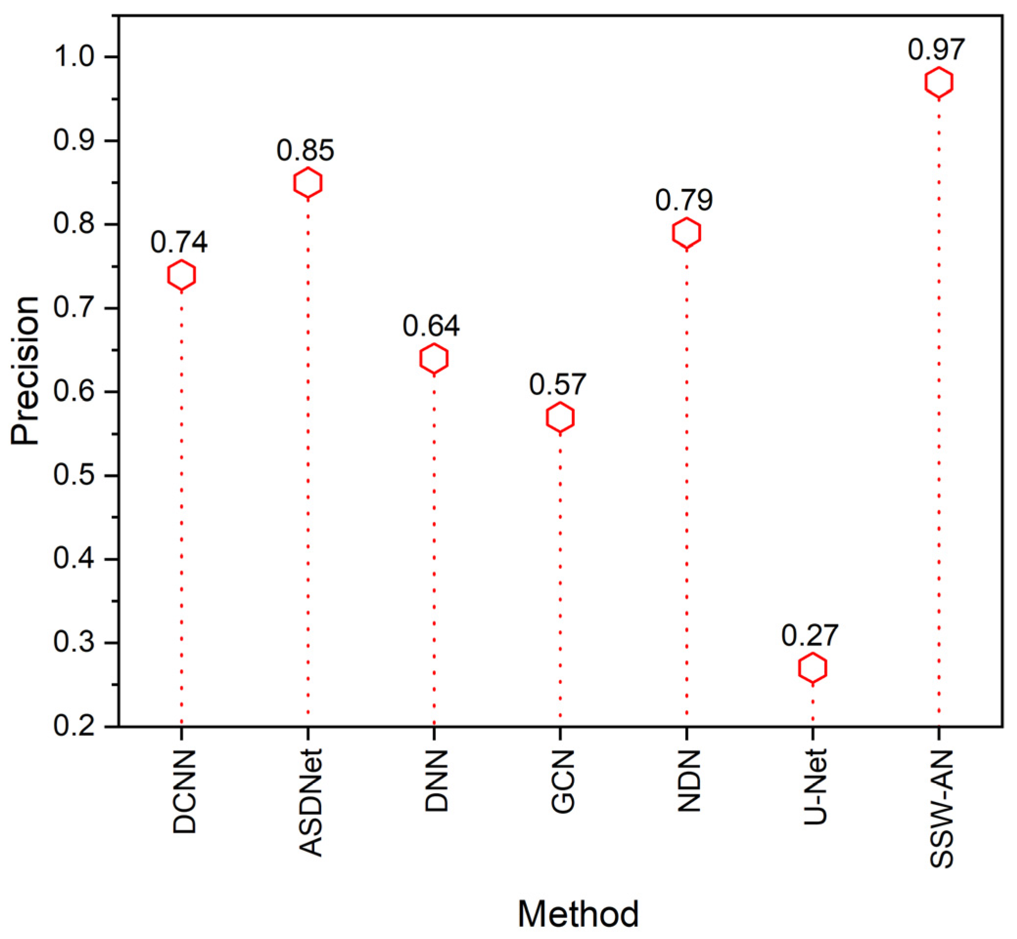
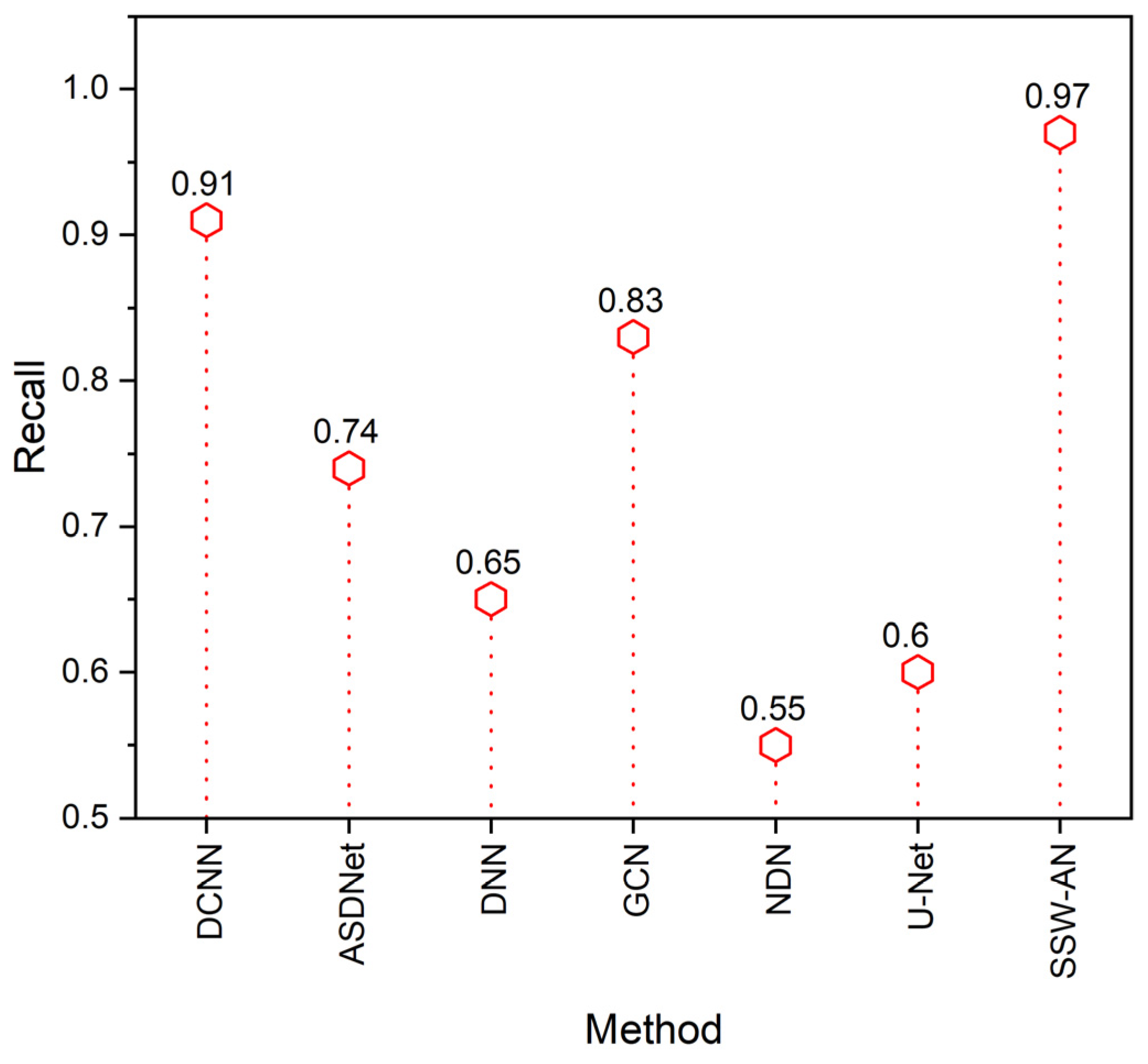
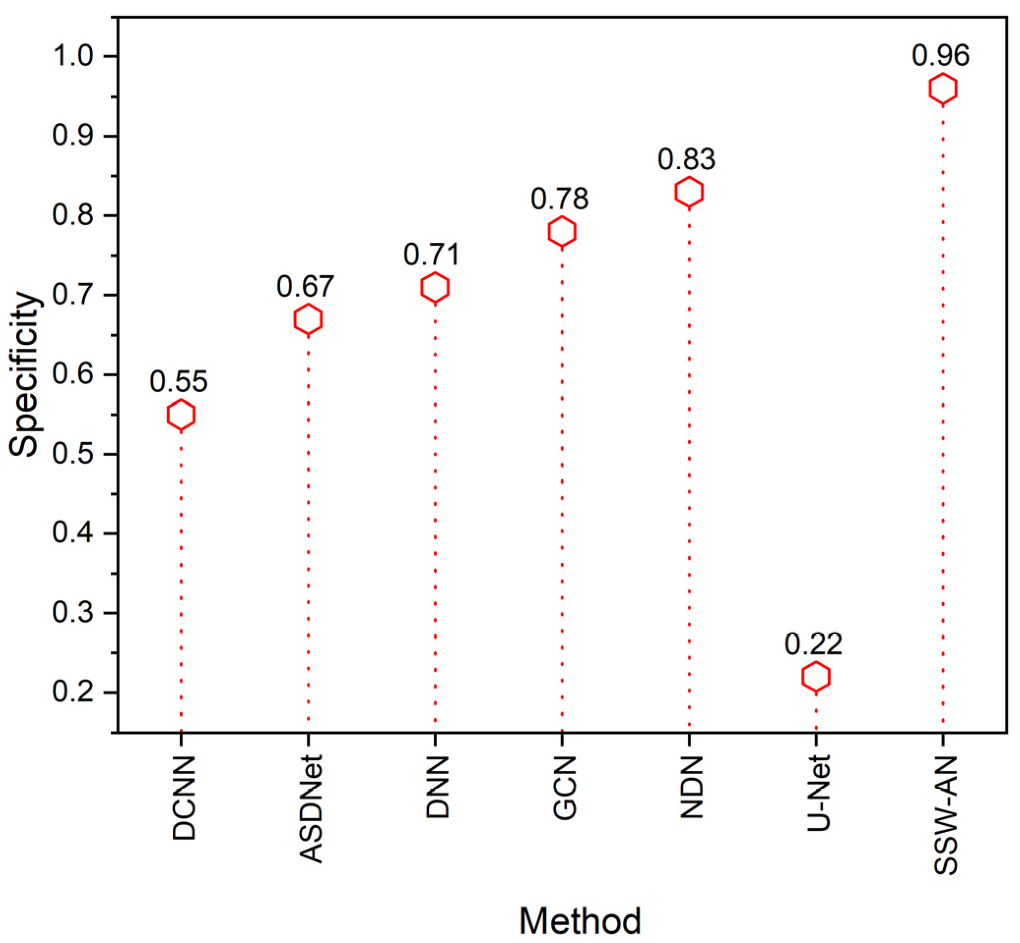
5.2. Discussion
6. Conclusions
Author Contributions
Funding
Institutional Review Board Statement
Informed Consent Statement
Data Availability Statement
Conflicts of Interest
References
- Li, S.; Zhang, C.; He, X. Shape-aware semi-supervised 3D semantic segmentation for medical images. In Medical Image Computing and Computer Assisted Intervention—MICCAI 2020; Springer International Publishing: Cham, Switzerland, 2020; pp. 552–561. [Google Scholar]
- Jin, K.; Huang, X.; Zhou, J.; Li, Y.; Yan, Y.; Sun, Y.; Zhang, Q.; Wang, Y.; Ye, J. FIVES: A fundus image dataset for artificial intelligence based vessel segmentation. Sci. Data 2022, 9, 475. [Google Scholar] [CrossRef] [PubMed]
- Xie, B.; Li, S.; Li, M.; Liu, C.H.; Huang, G.; Wang, G. SePiCo: Semantic-guided pixel contrast for domain adaptive semantic segmentation. IEEE Trans. Pattern Anal. Mach. Intell. 2023, 1–17. [Google Scholar] [CrossRef]
- Asgari Taghanaki, S.; Abhishek, K.; Cohen, J.P.; Cohen-Adad, J.; Hamarneh, G. Deep semantic segmentation of natural and medical images: A review. Artif. Intell. Rev. 2021, 54, 137–178. [Google Scholar] [CrossRef]
- Liu, L.; Wu, F.-X.; Wang, Y.-P.; Wang, J. Multi-receptive-field CNN for semantic segmentation of medical images. IEEE J. Biomed. Health Inform. 2020, 24, 3215–3225. [Google Scholar] [CrossRef]
- Ban, Y.; Wang, Y.; Liu, S.; Yang, B.; Liu, M.; Yin, L.; Zheng, W. 2D/3D multimode medical image alignment based on spatial histograms. Appl. Sci. 2022, 12, 8261. [Google Scholar] [CrossRef]
- Cheng, Z.; Qu, A.; He, X. Contour-aware semantic segmentation network with spatial attention mechanism for medical image. Vis. Comput. 2022, 38, 749–762. [Google Scholar] [CrossRef] [PubMed]
- Lu, H.; Wang, H.; Zhang, Q.; Yoon, S.W.; Won, D. A 3D convolutional neural network for volumetric image semantic segmentation. Procedia Manuf. 2019, 39, 422–428. [Google Scholar] [CrossRef]
- Alalwan, N.; Abozeid, A.; ElHabshy, A.A.; Alzahrani, A. Efficient 3D deep learning model for medical image semantic segmentation. Alex. Eng. J. 2021, 60, 1231–1239. [Google Scholar] [CrossRef]
- Fang, K.; Li, W.-J. DMNet: Difference minimization network for semi-supervised segmentation in medical images. In Medical Image Computing and Computer Assisted Intervention—MICCAI 2020; Springer International Publishing: Cham, Switzerland, 2020; pp. 532–541. [Google Scholar]
- Rezaei, M.; Yang, H.; Harmuth, K.; Meinel, C. Conditional generative adversarial refinement networks for unbalanced medical image semantic segmentation. In Proceedings of the 2019 IEEE Winter Conference on Applications of Computer Vision (WACV), Waikoloa Village, HI, USA, 7–11 January 2019. [Google Scholar]
- Rezaei, M.; Yang, H.; Meinel, C. Recurrent generative adversarial network for learning imbalanced medical image semantic segmentation. Multimed. Tools Appl. 2020, 79, 15329–15348. [Google Scholar] [CrossRef]
- Jiang, F.; Grigorev, A.; Rho, S.; Tian, Z.; Fu, Y.; Jifara, W.; Adil, K.; Liu, S. Medical image semantic segmentation based on deep learning. Neural Comput. Appl. 2018, 29, 1257–1265. [Google Scholar] [CrossRef]
- Petit, O.; Thome, N.; Charnoz, A.; Hostettler, A.; Soler, L. Handling missing annotations for semantic segmentation with deep ConvNets. In Deep Learning in Medical Image Analysis and Multimodal Learning for Clinical Decision Support; Springer International Publishing: Cham, Switzerland, 2018; pp. 20–28. [Google Scholar]
- Karayegen, G.; Aksahin, M.F. Brain tumor prediction on MR images with semantic segmentation by using deep learning network and 3D imaging of tumor region. Biomed. Signal Process. Control 2021, 66, 102458. [Google Scholar] [CrossRef]
- Xia, Y.; Zhang, Y.; Liu, F.; Shen, W.; Yuille, A.L. Synthesize then compare: Detecting failures and anomalies for semantic segmentation. In Computer Vision—ECCV 2020; Springer International Publishing: Cham, Switzerland, 2020; pp. 145–161. [Google Scholar]
- Wang, Z.; Zheng, J.-Q.; Voiculescu, I. An uncertainty-aware transformer for MRI cardiac semantic segmentation via mean teachers. In Medical Image Understanding and Analysis; Springer International Publishing: Cham, Switzerland, 2022; pp. 494–507. [Google Scholar]
- van Rijthoven, M.; Balkenhol, M.; Siliņa, K.; van der Laak, J.; Ciompi, F. HookNet: Multi-resolution convolutional neural networks for semantic segmentation in histopathology whole-slide images. Med. Image Anal. 2021, 68, 101890. [Google Scholar] [CrossRef] [PubMed]
- Yang, X.; Yu, L.; Li, S.; Wen, H.; Luo, D.; Bian, C.; Qin, J.; Ni, D.; Heng, P.-A. Towards automated semantic segmentation in prenatal volumetric ultrasound. IEEE Trans. Med. Imaging 2019, 38, 180–193. [Google Scholar] [CrossRef] [PubMed]
- Ali, M.; Gilani, S.O.; Waris, A.; Zafar, K.; Jamil, M. Brain tumour image segmentation using deep networks. IEEE Access 2020, 8, 153589–153598. [Google Scholar] [CrossRef]
- Kumar, D.M.; Satyanarayana, D.; Prasad, M.N.G. An improved Gabor wavelet transform and rough K-means clustering algorithm for MRI brain tumor image segmentation. Multimed. Tools Appl. 2021, 80, 6939–6957. [Google Scholar] [CrossRef]
- Wang, W.; Chen, C.; Ding, M.; Yu, H.; Zha, S.; Li, J. TransBTS: Multimodal brain tumor segmentation using transformer. In Medical Image Computing and Computer Assisted Intervention—MICCAI 2021; Springer International Publishing: Cham, Switzerland, 2021; pp. 109–119. [Google Scholar]
- Wadhwa, A.; Bhardwaj, A.; Singh Verma, V. A review on brain tumor segmentation of MRI images. Magn. Reson. Imaging 2019, 61, 247–259. [Google Scholar] [CrossRef]
- Zhao, Y.-X.; Zhang, Y.-M.; Liu, C.-L. Bag of tricks for 3D MRI brain tumor segmentation. In Brainlesion: Glioma, Multiple Sclerosis, Stroke and Traumatic Brain Injuries; Springer International Publishing: Cham, Switzerland, 2020; pp. 210–220. [Google Scholar]
- Liu, X.; Wang, S.; Lin, J.C.-W.; Liu, S. An algorithm for overlapping chromosome segmentation based on region selection. Neural Comput. Appl. 2022, 1–10. [Google Scholar] [CrossRef]
- Bruno, P.; Calimeri, F.; Marte, C.; Manna, M. Combining deep learning and ASP-based models for the semantic segmentation of medical images. In Rules and Reasoning; Springer International Publishing: Cham, Switzerland, 2021; pp. 95–110. [Google Scholar]
- Emara, T.; Munim, H.E.A.E.; Abbas, H.M. LiteSeg: A novel lightweight ConvNet for semantic segmentation. In Proceedings of the 2019 Digital Image Computing: Techniques and Applications (DICTA), Perth, Australia, 2–4 December 2019. [Google Scholar]
- Qin, Y.; Kamnitsas, K.; Ancha, S.; Nanavati, J.; Cottrell, G.; Criminisi, A.; Nori, A. Autofocus Layer for Semantic Segmentation. In Medical Image Computing and Computer Assisted Intervention—MICCAI 2018; Springer International Publishing: Cham, Switzerland, 2018; pp. 603–611. [Google Scholar]
- Fang, F.; Yao, Y.; Zhou, T.; Xie, G.; Lu, J. Self-supervised multi-modal hybrid fusion network for brain tumor segmentation. IEEE J. Biomed. Health Inform. 2022, 26, 5310–5320. [Google Scholar] [CrossRef]
- Ding, Y.; Gong, L.; Zhang, M.; Li, C.; Qin, Z. A multi-path adaptive fusion network for multimodal brain tumor segmentation. Neurocomputing 2020, 412, 19–30. [Google Scholar] [CrossRef]
- Jiang, Y.; Ye, M.; Wang, P.; Huang, D.; Lu, X. MRF-IUNet: A multiresolution fusion brain tumor segmentation network based on improved inception U-Net. Comput. Math. Methods Med. 2022, 2022, 6305748. [Google Scholar] [CrossRef]
- Zhou, T.; Ruan, S.; Guo, Y.; Canu, S. A multi-modality fusion network based on attention mechanism for brain tumor segmentation. In Proceedings of the 2020 IEEE 17th International Symposium on Biomedical Imaging (ISBI), Iowa City, IA, USA, 3–7 April 2020. [Google Scholar]
- Liu, X.; Xing, F.; El Fakhri, G.; Woo, J. Self-semantic contour adaptation for cross modality brain tumor segmentation. In Proceedings of the 2022 IEEE 19th International Symposium on Biomedical Imaging (ISBI), Kolkata, India, 28–31 March 2022. [Google Scholar]
- Liu, H.; Liu, M.; Li, D.; Zheng, W.; Yin, L.; Wang, R. Recent advances in pulse-coupled neural networks with applications in image processing. Electronics 2022, 11, 3264. [Google Scholar] [CrossRef]
- Kalinin, A.A.; Iglovikov, V.I.; Rakhlin, A.; Shvets, A.A. Medical image segmentation using deep neural networks with pre-trained encoders. In Advances in Intelligent Systems and Computing; Springer Singapore: Singapore, 2020; pp. 39–52. [Google Scholar]
- Hatamizadeh, A.; Nath, V.; Tang, Y.; Yang, D.; Roth, H.R.; Xu, D. Swin UNETR: Swin transformers for semantic segmentation of brain tumors in MRI images. In Brainlesion: Glioma, Multiple Sclerosis, Stroke and Traumatic Brain Injuries; Springer International Publishing: Cham, Switzerland, 2022; pp. 272–284. [Google Scholar]
- Jha, D.; Riegler, M.A.; Johansen, D.; Halvorsen, P.; Johansen, H.D. DoubleU-net: A deep convolutional neural network for medical image segmentation. In Proceedings of the 2020 IEEE 33rd International Symposium on Computer-Based Medical Systems (CBMS), Rochester, MN, USA, 28–30 July 2020. [Google Scholar]
- Nie, D.; Gao, Y.; Wang, L.; Shen, D. ASDNet: Attention based semi-supervised deep networks for medical image segmentation. In Medical Image Computing and Computer Assisted Intervention—MICCAI 2018; Springer International Publishing: Cham, Switzerland, 2018; pp. 370–378. [Google Scholar]
- Ni, J.; Wu, J.; Tong, J.; Chen, Z.; Zhao, J. GC-Net: Global context network for medical image segmentation. Comput. Methods Programs Biomed. 2020, 190, 105121. [Google Scholar] [CrossRef] [PubMed]
- Wang, L.; Chen, R.; Wang, S.; Zeng, N.; Huang, X.; Liu, C. Nested dilation network (NDN) for multi-task medical image segmentation. IEEE Access 2019, 7, 44676–44685. [Google Scholar] [CrossRef]
- Siddique, N.; Paheding, S.; Elkin, C.P.; Devabhaktuni, V. U-net and its variants for medical image segmentation: A review of theory and applications. IEEE Access 2021, 9, 82031–82057. [Google Scholar] [CrossRef]


Disclaimer/Publisher’s Note: The statements, opinions and data contained in all publications are solely those of the individual author(s) and contributor(s) and not of MDPI and/or the editor(s). MDPI and/or the editor(s) disclaim responsibility for any injury to people or property resulting from any ideas, methods, instructions or products referred to in the content. |
© 2023 by the authors. Licensee MDPI, Basel, Switzerland. This article is an open access article distributed under the terms and conditions of the Creative Commons Attribution (CC BY) license (https://creativecommons.org/licenses/by/4.0/).
Share and Cite
Anusooya, G.; Bharathiraja, S.; Mahdal, M.; Sathyarajasekaran, K.; Elangovan, M. Self-Supervised Wavelet-Based Attention Network for Semantic Segmentation of MRI Brain Tumor. Sensors 2023, 23, 2719. https://doi.org/10.3390/s23052719
Anusooya G, Bharathiraja S, Mahdal M, Sathyarajasekaran K, Elangovan M. Self-Supervised Wavelet-Based Attention Network for Semantic Segmentation of MRI Brain Tumor. Sensors. 2023; 23(5):2719. https://doi.org/10.3390/s23052719
Chicago/Turabian StyleAnusooya, Govindarajan, Selvaraj Bharathiraja, Miroslav Mahdal, Kamsundher Sathyarajasekaran, and Muniyandy Elangovan. 2023. "Self-Supervised Wavelet-Based Attention Network for Semantic Segmentation of MRI Brain Tumor" Sensors 23, no. 5: 2719. https://doi.org/10.3390/s23052719