Author Contributions
Conceptualization, A.D. and K.K.; methodology, A.D., A.I., M.S. and K.K.; software, A.D., A.I. and M.S.; validation, J.P., S.T. and A.K.; formal analysis, K.K. and F.A.M.; investigation, K.K., J.P., S.T. and A.K.; resources, A.D., A.I. and M.S.; data curation, A.D., A.I. and M.S.; writing—original draft preparation, A.D.; writing—review and editing, K.K. and F.A.M.; visualization, A.I. and M.S.; supervision, K.K. and F.A.M.; project administration, J.P., S.T. and A.K.; funding acquisition, J.P., S.T. and A.K. All authors have read and agreed to the published version of the manuscript.
Figure 1.
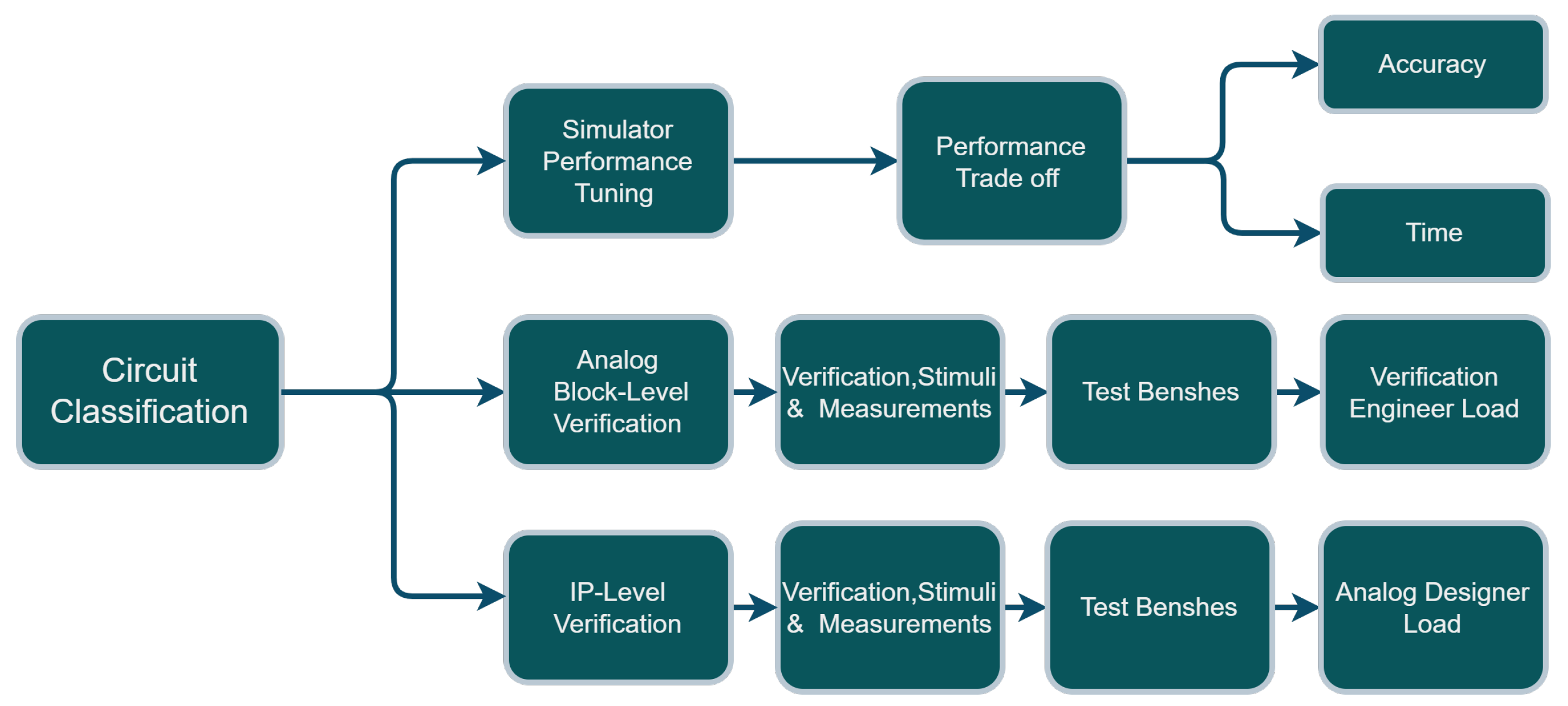
Circuit classification use cases: Simulator performance tuning, analog block-level verification, and IP-level verification.
Figure 1.
Circuit classification use cases: Simulator performance tuning, analog block-level verification, and IP-level verification.
Figure 2.
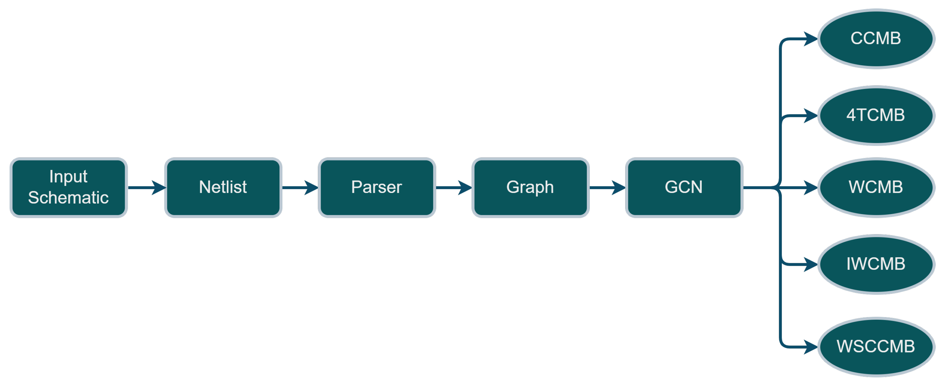
Overall system PIPELINE of the developed Analog Circuit Classifier. An input schematic is converted to a graph model through a parser we have developed. Then, the equivalent graph model is fed into the GCN to be classified into one of the following classes: Cascode Current Mirror Bank (CCMB), 4 Transistor Current Mirror Bank (4TCMB), Wilson Current Mirror Bank (WCMB), Improved Wilson Current Mirror Bank (IWCMB), Wide Swing Cascode Current Mirror Bank (WSCCMB).
Figure 2.
Overall system PIPELINE of the developed Analog Circuit Classifier. An input schematic is converted to a graph model through a parser we have developed. Then, the equivalent graph model is fed into the GCN to be classified into one of the following classes: Cascode Current Mirror Bank (CCMB), 4 Transistor Current Mirror Bank (4TCMB), Wilson Current Mirror Bank (WCMB), Improved Wilson Current Mirror Bank (IWCMB), Wide Swing Cascode Current Mirror Bank (WSCCMB).
Figure 3.
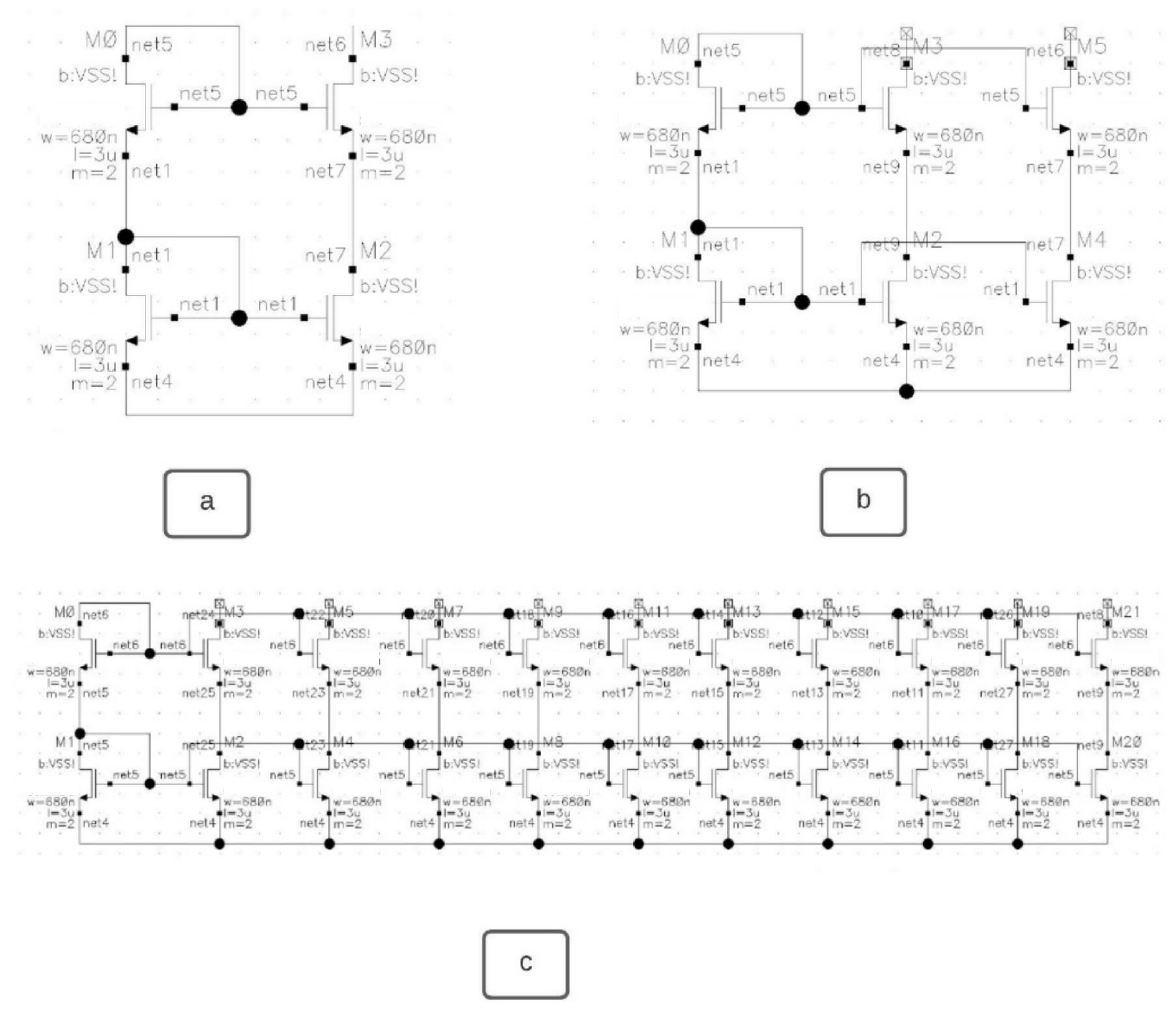
Example schematics samples of the same class “cascode current mirror bank (CCMB”). Different configurations are presented here: (a) 0 bank; (b) 1 bank; and (c) 9 banks. For each other class (in total we have 5 classes) within the dataset, there are similarly 10 topology/architecture variations.
Figure 3.
Example schematics samples of the same class “cascode current mirror bank (CCMB”). Different configurations are presented here: (a) 0 bank; (b) 1 bank; and (c) 9 banks. For each other class (in total we have 5 classes) within the dataset, there are similarly 10 topology/architecture variations.
Figure 4.
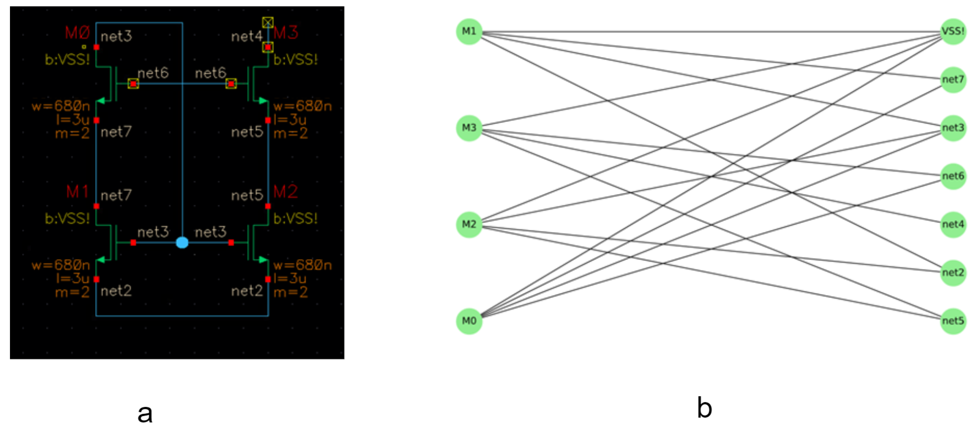
(a) An NMOS current mirror of four transistors. (b) its representation as a bipartite graph.
Figure 4.
(a) An NMOS current mirror of four transistors. (b) its representation as a bipartite graph.
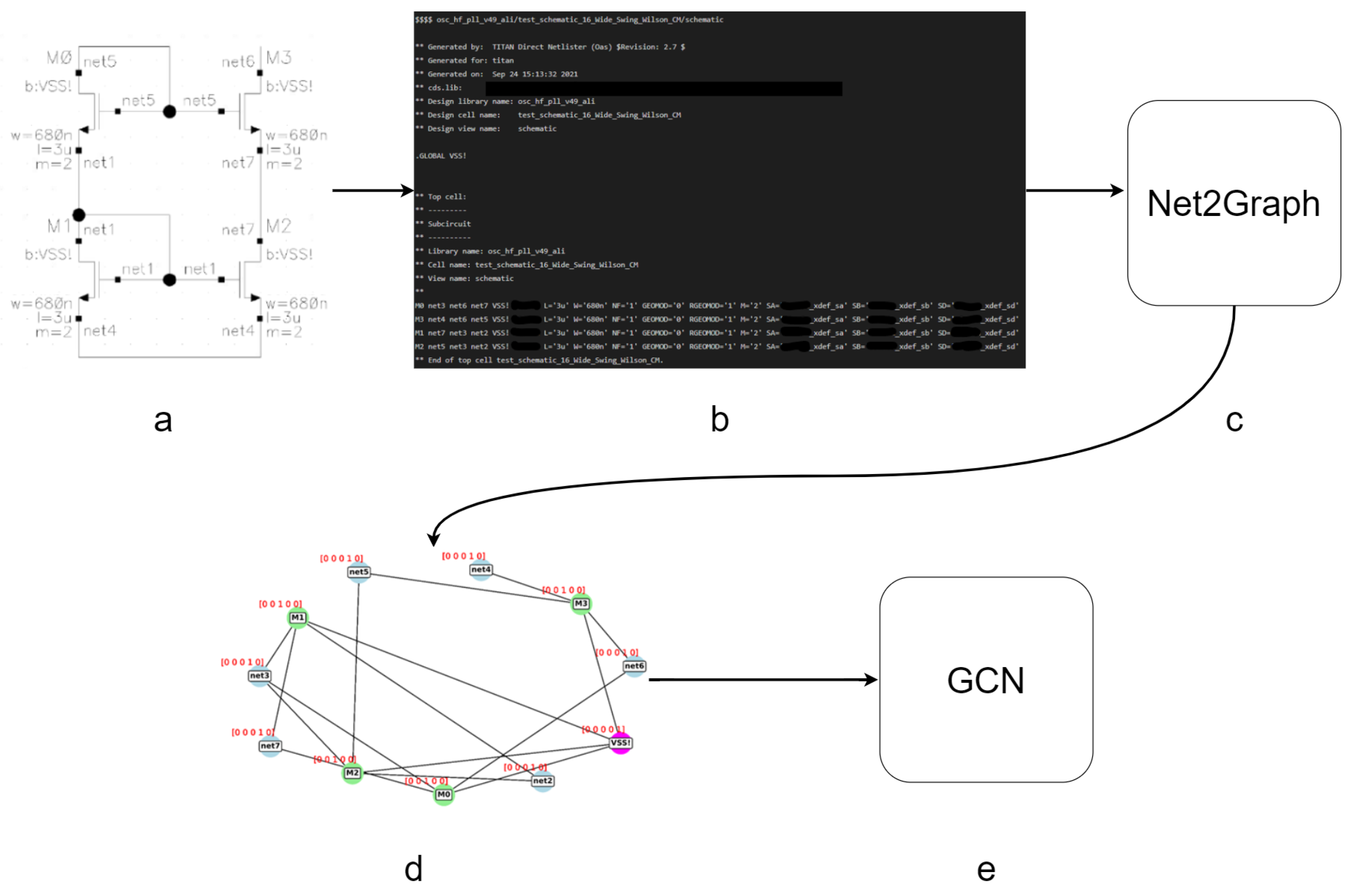
Figure 5.
System overview: a pipeline for one sample classification using GCN. (a) Input schematic, (b) the schematic is converted to Spice netlist using Cadence Virtuoso, (c) Spice netlist parser, (d) the parser is used to convert the netlist into a graph, (e) GCN is the chosen neural network model to perform the classification.
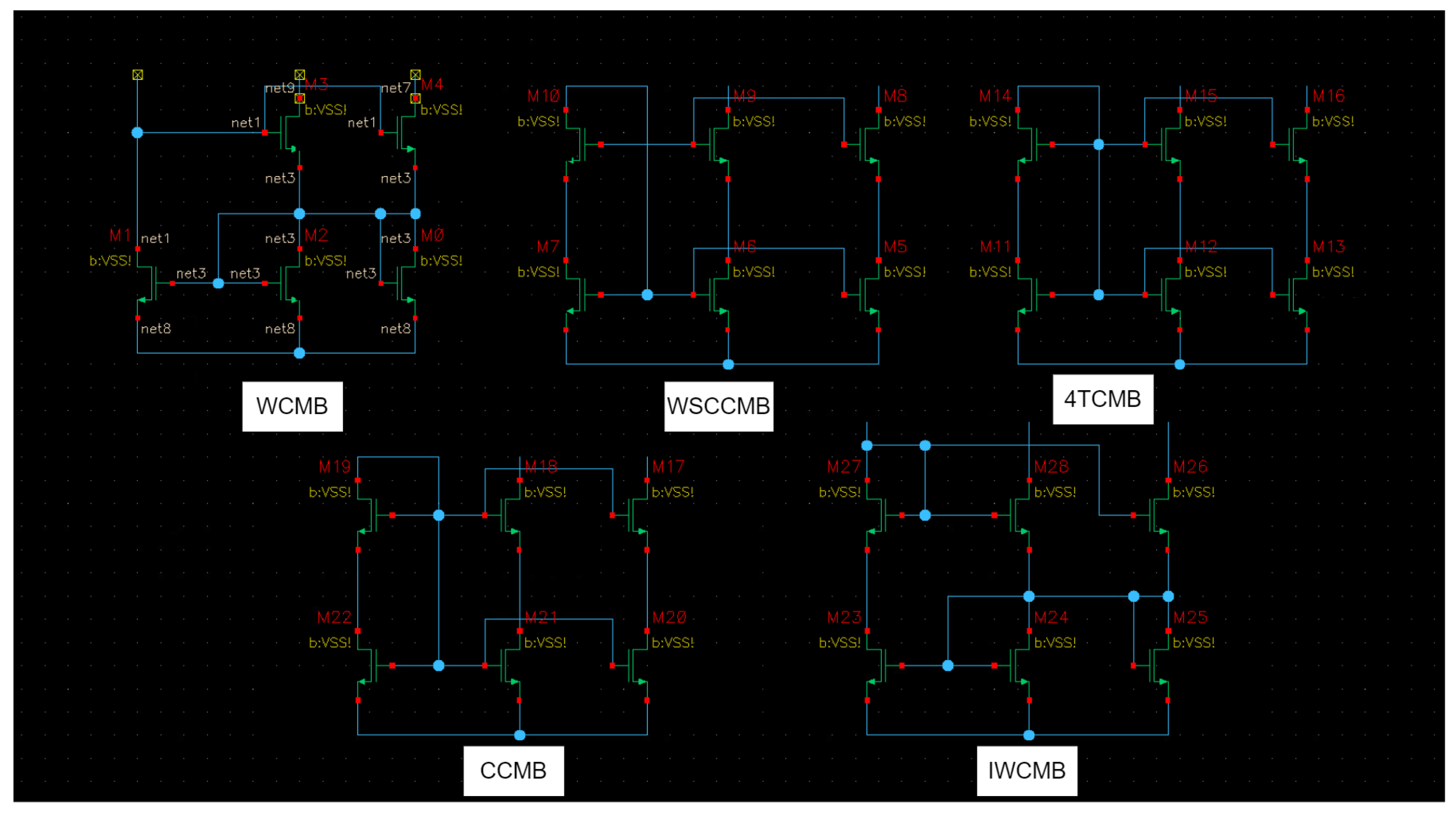
Figure 6.
Five classes of current mirror banks to be classified: Cascode Current Mirror Bank(CCMB), 4 Transistor Current Mirror Bank (4TCMB), Wilson Current Mirror Bank (WCMB), Improved Wilson Current Mirror Bank (IWCMB), Wide Swing Cascode Current Mirror Bank (WSCCMB). Each one has an extra bank and the possibility to add more banks on the right side [
24].
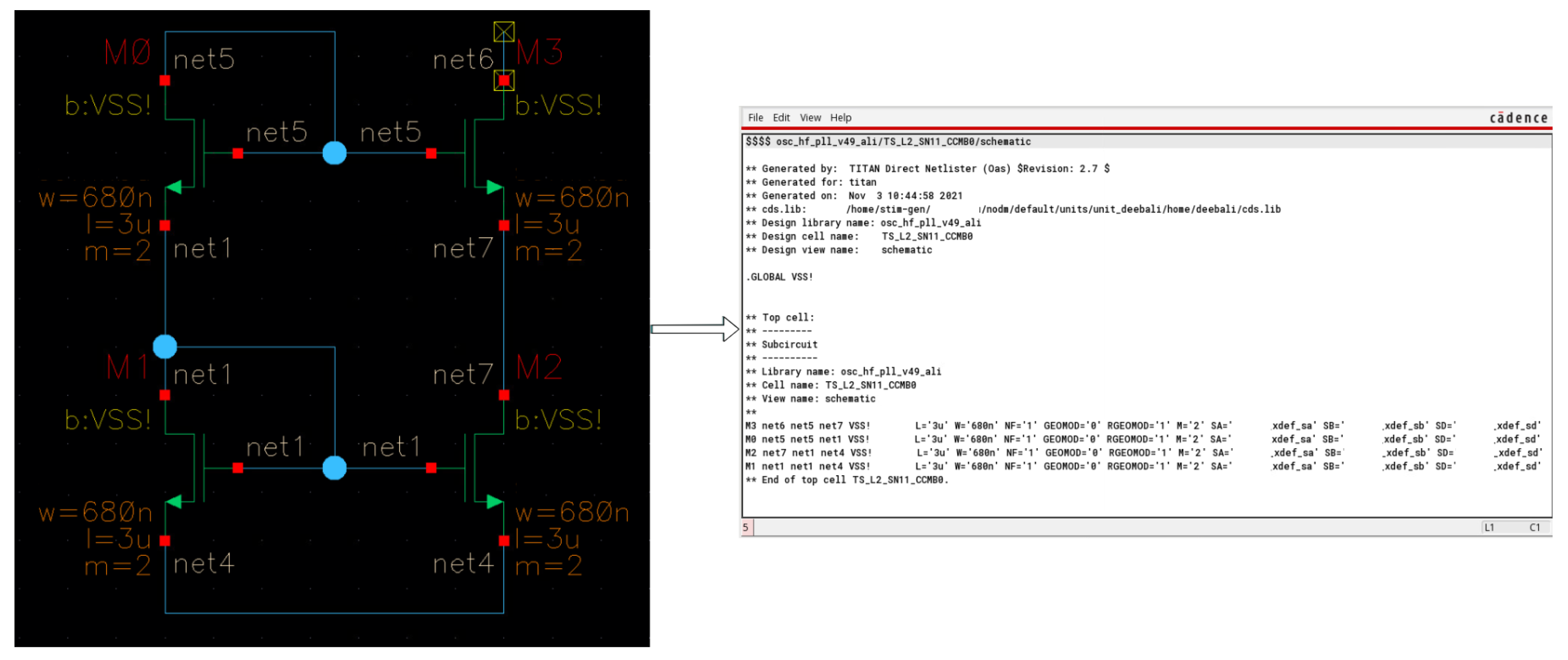
Figure 7.
Dataset Transformation: Converting schematics to netlists using Cadence Virtuoso. The connectivity of the transistors is described after each transistor name in text form, followed by the electrical description and characterization of each transistor.
Figure 7.
Dataset Transformation: Converting schematics to netlists using Cadence Virtuoso. The connectivity of the transistors is described after each transistor name in text form, followed by the electrical description and characterization of each transistor.
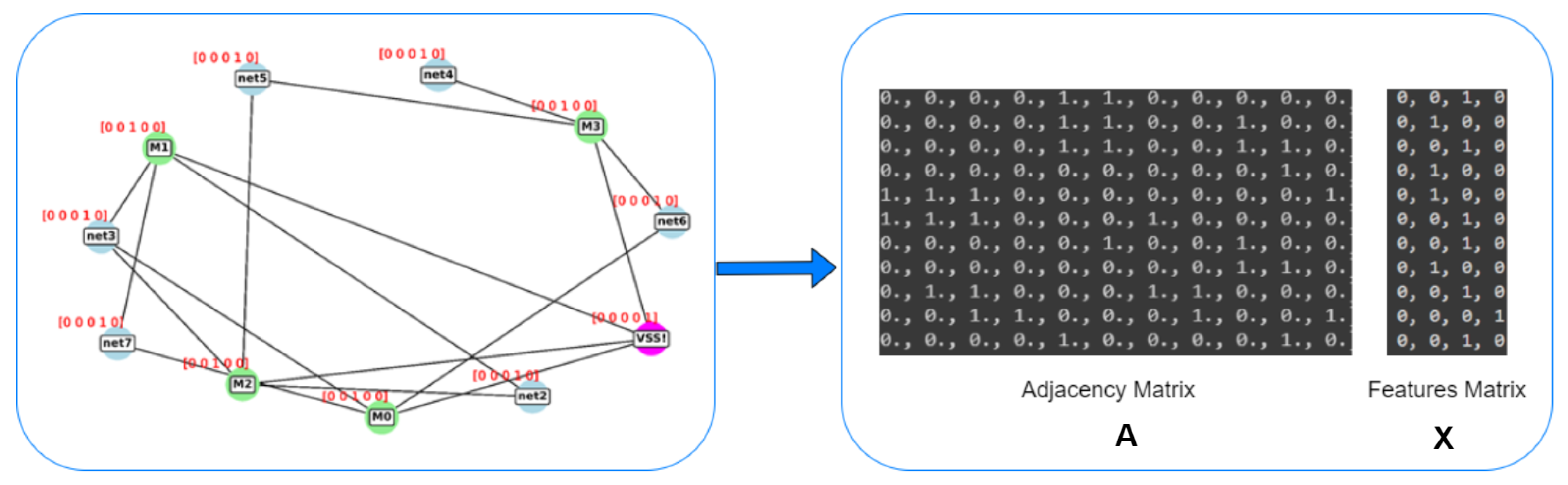
Figure 8.
Dataset preprocessing: Converting the netlist to annotated graphs, then representing each graph with adjacency and feature matrices.
Figure 8.
Dataset preprocessing: Converting the netlist to annotated graphs, then representing each graph with adjacency and feature matrices.
Figure 9.
The architecture of the GCN classifier model. Using the fast approximation of spectral convolution, H1 and H2 are the output of the first and second convolution layers, calculated using
, the normalized Adjacency matrix [
41], a. ReLU layers remove the negative values, and finally, the SoftMax layer votes for the detected class.
Figure 10.
Kfold cross-validation mechanism: in each iteration, a part of the dataset is used for testing the model while the rest is used for training the model independently. In other iterations, another part is used for testing, and so on [
56].
Figure 10.
Kfold cross-validation mechanism: in each iteration, a part of the dataset is used for testing the model while the rest is used for training the model independently. In other iterations, another part is used for testing, and so on [
56].
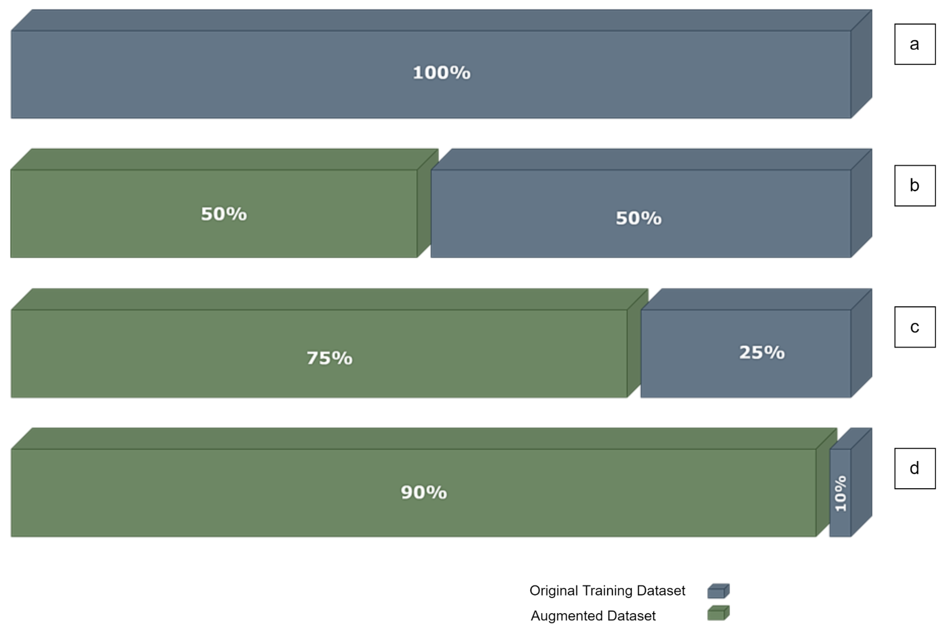
Figure 11.
(a) Training dataset TDS. (b) TDS/2: 50% of the training dataset and 50% augmented data. (c) TDS/4: 25% of the training dataset and 75% augmented data. (d) TDS/10: 10% of the training dataset and 90% augmented data.
Figure 11.
(a) Training dataset TDS. (b) TDS/2: 50% of the training dataset and 50% augmented data. (c) TDS/4: 25% of the training dataset and 75% augmented data. (d) TDS/10: 10% of the training dataset and 90% augmented data.
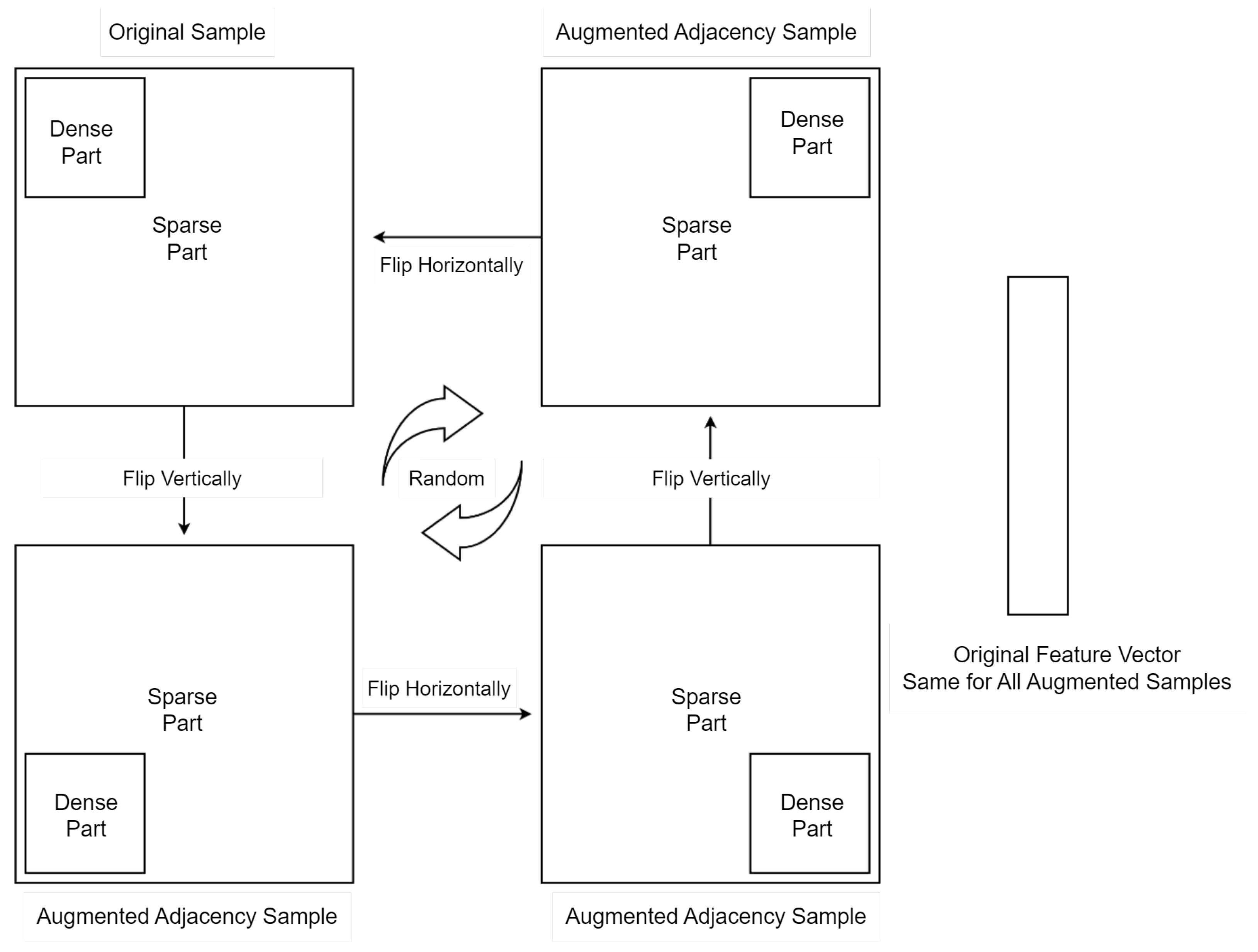
Figure 12.
For each adjacency matrix in the training set, the dense part is flipped systematically and the original feature vector is fixed for all augmented samples. Then we extend the training dataset with the new augmented adjacency matrix concatenated with the original feature vector as follows [Adj Augmented | X Original].
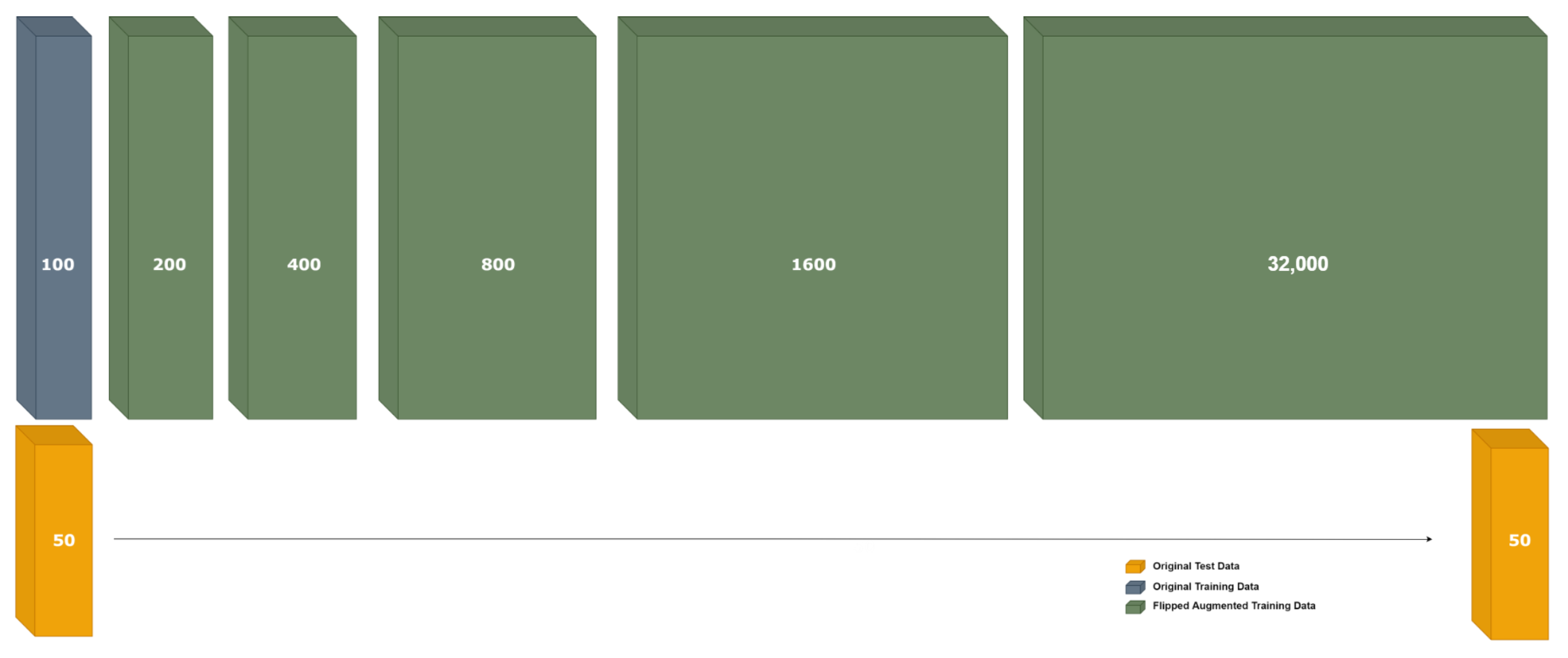
Figure 13.
Augmentation by flipping: Original test dataset was kept the same. On the other hand, the training dataset was augmented from 100 graphs up to 32,000 graphs through 5 stages.
Figure 13.
Augmentation by flipping: Original test dataset was kept the same. On the other hand, the training dataset was augmented from 100 graphs up to 32,000 graphs through 5 stages.
Figure 14.
Augmentation by flipping: Original test dataset was kept the same. On the other hand, the training dataset was augmented from 100 graphs up to 32,000 graphs through 5 stages.
Figure 14.
Augmentation by flipping: Original test dataset was kept the same. On the other hand, the training dataset was augmented from 100 graphs up to 32,000 graphs through 5 stages.
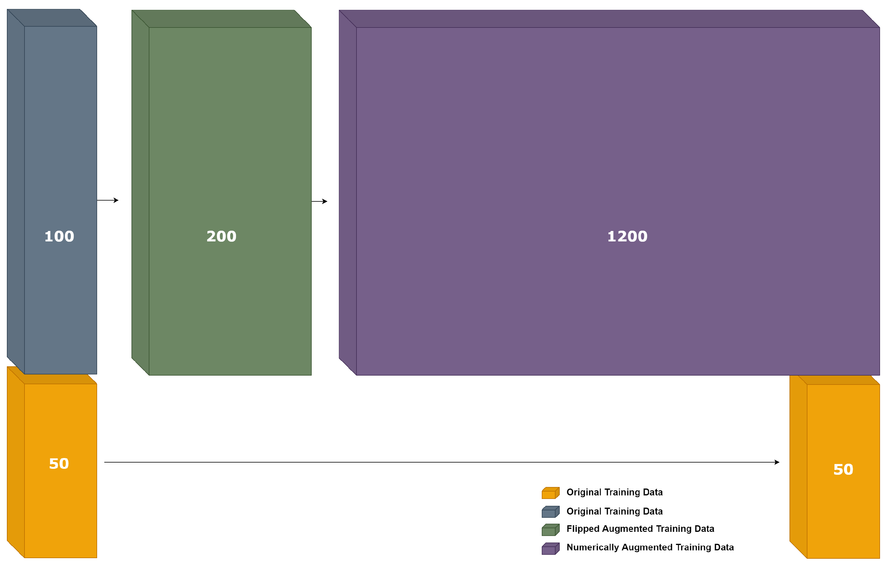
Figure 15.
Multistage augmentation visualization: Data augmented first by flipping and then numerically.
Figure 15.
Multistage augmentation visualization: Data augmented first by flipping and then numerically.
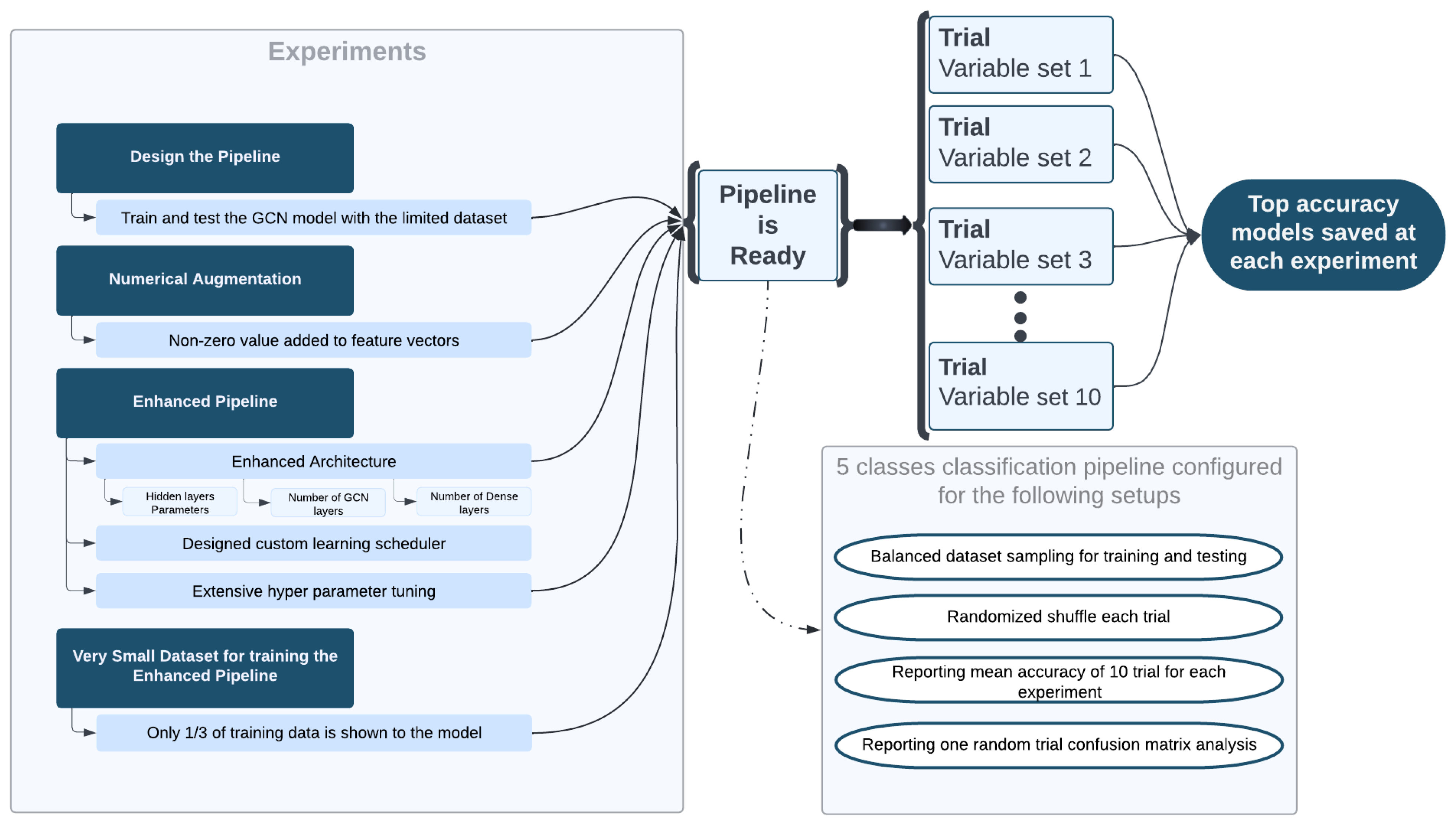
Figure 16.
Block diagram of the experiments anatomy of the pipelines for describing the progress until developing the finally used best pipeline.
Figure 16.
Block diagram of the experiments anatomy of the pipelines for describing the progress until developing the finally used best pipeline.
Table 1.
An overview of the most relevant related works w.r.t. an assessment of how far they do satisfy the six requirements formulated and outlined in
Section 2 (see Requirements Engineering dossier).
Table 1.
An overview of the most relevant related works w.r.t. an assessment of how far they do satisfy the six requirements formulated and outlined in
Section 2 (see Requirements Engineering dossier).
| Most Relevant Related Works | Classification Accuracy in Range 97–99% (REQ-1) | Robustness w.r.t. Architecture Variations (REQ-2) | Robustness w.r.t. Architecture Extension through Banks (REQ-3) | Robustness w.r.t. Transistor Technologies Variations (REQ.4) | Robustness w.r.t. Training Dataset Imperfections (REQ-5) | Applicability to Higher Levels of AMS IP Stacks |
|---|
| Kunal et al. [4] | Yes | Yes | No | No | No | Yes, possibly |
| Hong et al. [5] | Yes | Yes | No | No | No | Yes, possibly |
| Zhang et al. [19] | Yes | Yes | No | No | No | Yes, possibly |
| Ahmad et al. [24] | Yes | Yes | No | No | No | Yes, possibly |
Table 2.
Created dataset in Cadence Virtuoso: For each class of current mirror banks, 10 schematics were created by adding more banks. The first sample was created with no banks at all, and the last one was created with nine banks.
Table 2.
Created dataset in Cadence Virtuoso: For each class of current mirror banks, 10 schematics were created by adding more banks. The first sample was created with no banks at all, and the last one was created with nine banks.
| Wide Swing Cascode Current Mirror Bank | Cascode Current Mirror Bank | 4 Transistor Current Mirror Bank | Wilson Current Mirror Bank | Improved Wilson Current Mirror Bank |
|---|
| TS_L2_SN1_WSCCMB0 | TS_L2_SN11_CCMB0 | TS_L2_SN21_4TCMB0 | TS_L2_SN31_WCMB0 | TS_L2_SN41_ IWCMB0 |
| TS_L2_SN2_WSCCMB1 | TS_L2_SN12_CCMB1 | TS_L2_SN22_4TCMB1 | TS_L2_SN32_WCMB1 | TS_L2_SN42_ IWCMB1 |
| TS_L2_SN3_WSCCMB2 | TS_L2_SN13_CCMB2 | TS_L2_SN23_4TCMB2 | TS_L2_SN33_WCMB2 | TS_L2_SN43_ IWCMB2 |
| TS_L2_SN4_WSCCMB3 | TS_L2_SN14_CCMB3 | TS_L2_SN24_4TCMB3 | TS_L2_SN34_WCMB3 | TS_L2_SN44_ IWCMB3 |
| TS_L2_SN5_WSCCMB4 | TS_L2_SN15_CCMB4 | TS_L2_SN25_4TCMB4 | TS_L2_SN35_WCMB4 | TS_L2_SN45_ IWCMB4 |
| TS_L2_SN6_WSCCMB5 | TS_L2_SN16_CCMB5 | TS_L2_SN26_4TCMB5 | TS_L2_SN36_WCMB5 | TS_L2_SN46_ IWCMB5 |
| TS_L2_SN7_WSCCMB6 | TS_L2_SN17_CCMB6 | TS_L2_SN27_4TCMB6 | TS_L2_SN37_ WCMB6 | TS_L2_SN47_ IWCMB6 |
| TS_L2_SN8_WSCCMB7 | TS_L2_SN18_CCMB7 | TS_L2_SN28_4TCMB7 | TS_L2_SN38_ WCMB7 | TS_L2_SN48_ IWCMB7 |
| TS_L2_SN9_WSCCMB8 | TS_L2_SN19_CCMB8 | TS_L2_SN29_4TCMB8 | TS_L2_SN39_ WCMB8 | TS_L2_SN49_ IWCMB8 |
| TS_L2_SN10_WSCCMB9 | TS_L2_SN20_CCMB9 | TS_L2_SN30_4TCMB9 | TS_L2_SN40_ WCMB9 | TS_L2_SN50_ IWCMB9 |
Table 3.
Five unique types of elements are considered for this classification problem.
Table 3.
Five unique types of elements are considered for this classification problem.
| Node Type | Feature Vector |
|---|
| NMOS [CMOS] | [0 1 0 0 0] |
| PMOS [CMOS] | [0 0 1 0 0] |
| BIPOLAR | [1 0 0 0 0] |
| N- Voltage Source | [0 0 0 0 1] |
| N-Net | [0 0 0 1 0] |
Table 4.
K-Fold (5 folds case): 1/5 of the dataset is used for testing and the rest is used for training. A confusion matrix is drawn for each one of the five folds. They show 100% accuracy for fold 4, and 90% accuracy for fold 3.
Table 4.
K-Fold (5 folds case): 1/5 of the dataset is used for testing and the rest is used for training. A confusion matrix is drawn for each one of the five folds. They show 100% accuracy for fold 4, and 90% accuracy for fold 3.
| Score for fold 1—Accuracy of 100% |
| True labels | 4TCM | 100% (9/9) | | | | |
| WCM | | 100% (4/4) | | | |
| WSCCM | | | 100% (6/6) | | |
| IWCM | | | | 100% (6/6) | |
| CCM | | | | | 100% (5/5) |
| | | 4TCM | WCM | WSCCM | IWCM | CCM |
| | | Predicted labels |
| Score for fold 2—Accuracy of 100% |
| True labels | 4TCM | 100% (8/8) | | | | |
| WCM | | 100% (9/9) | | | |
| WSCCM | | | 100% (3/3) | | |
| IWCM | | | | 100% (6/6) | |
| CCM | | | | | 100% (4/4) |
| | | 4TCM | WCM | WSCCM | IWCM | CCM |
| | | Predicted labels |
| Score for fold 3— Accuracy of 90% |
| True labels | 4TCM | 100% (3/3) | | | | |
| WCM | | 100% (8/8) | | | |
| WSCCM | 30% (3) | | 100% (7/10) | | |
| IWCM | | | | 100% (2/2) | |
| CCM | | | | | 100% (7/7) |
| | | 4TCM | WCM | WSCCM | IWCM | CCM |
| | | Predicted labels |
| Score for fold 4—Accuracy of 100% |
| True labels | 4TCM | 100% (5/5) | | | | |
| WCM | | 100% (3/3) | | | |
| WSCCM | | | 100% (4/4) | | |
| IWCM | | | | 100% (9/9) | |
| CCM | | | | | 100% (9/9) |
| | | 4TCM | WCM | WSCCM | IWCM | CCM |
| | | Predicted labels |
| Score for fold 5—Accuracy of 100% |
| True labels | 4TCM | 100% (5/5) | | | | |
| WCM | | 100% (6/6) | | | |
| WSCCM | | | 100% (7/7) | | |
| IWCM | | | | 100% (7/7) | |
| CCM | | | | | 100% (5/5) |
| | | 4TCM | WCM | WSCCM | IWCM | CCM |
| | | Predicted labels |
Table 5.
A total of 15 folds were applied on the dataset, which means in each fold 1/15 of the dataset is used for testing and the rest 14/15 is used for training independently. For each fold, a confusion matrix is drawn, and all confusion matrices show 100% accuracy of detection.
Table 5.
A total of 15 folds were applied on the dataset, which means in each fold 1/15 of the dataset is used for testing and the rest 14/15 is used for training independently. For each fold, a confusion matrix is drawn, and all confusion matrices show 100% accuracy of detection.
| Score for fold 1—Accuracy of 100% |
| True labels | 4TCM | 100% (4/4) | | | | |
| WCM | | 100% (2/2) | | | |
| WSCCM | | | 100% (2/2) | | |
| IWCM | | | | 100% (2/2) | |
| | | 4TCM | WCM | WSCCM | IWCM | |
| | | Predicted labels | |
| Score for fold 2—Accuracy of 100% |
| True labels | 4TCM | 100% (5/5) | | | | |
| WCM | | 100% (2/2) | | | |
| WSCCM | | | 100% (3/3) | | |
| | | 4TCM | WCM | WSCCM | | |
| | | Predicted labels | | |
| Score for fold 3—Accuracy of 100% |
| True labels | 4TCM | 100% (1/1) | | | | |
| WCM | | 100% (1/1) | | | |
| WSCCM | | | 100% (6/6) | | |
| IWCM | | | | 100% (2/2) | |
| | | 4TCM | WCM | WSCCM | IWCM | |
| | | Predicted labels | |
| Score for fold 4—Accuracy of 100% |
| True labels | 4TCM | 100% (6/6) | | | | |
| WCM | | 100% (4/4) | | | |
| | | 4TCM | WCM | | | |
| | | Predicted labels | |
| Score for fold 5—Accuracy of 100% |
| True labels | 4TCM | 100% (4/4) | | | | |
| WCM | | 100% (2/2) | | | |
| WSCCM | | | 100% (3/3) | | |
| IWCM | | | | 100% (1/1) | |
| | | 4TCM | WCM | WSCCM | IWCM | |
| | | Predicted labels | |
| Score for fold 6—Accuracy of 100% |
| True labels | 4TCM | 100% (3/3) | | | | |
| WCM | | 100% (1/1) | | | |
| WSCCM | | | 100% (2/2) | | |
| IWCM | | | | 100% (2/2) | |
| CCM | | | | | 100% (2/2) |
| | | 4TCM | WCM | WSCCM | IWCM | CCM |
| | | Predicted labels |
| Score for fold 7—Accuracy of 100% |
| True labels | 4TCM | 100% (1/1) | | | | |
| WCM | | 100% (2/2) | | | |
| WSCCM | | | 100% (1/1) | | |
| IWCM | | | | 100% (2/2) | |
| CCM | | | | | 100% (4/4) |
| | | 4TCM | WCM | WSCCM | IWCM | CCM |
| | | Predicted labels |
| Score for fold 8—Accuracy of 100% |
| True labels | 4TCM | 100% (1/1) | | | | |
| WCM | | 100% (1/1) | | | |
| WSCCM | | | 100% (3/3) | | |
| IWCM | | | | 100% (3/3) | |
| CCM | | | | | 100% (2/2) |
| | | 4TCM | WCM | WSCCM | IWCM | CCM |
| | | Predicted labels |
| Score for fold 9—Accuracy of 100% |
| True labels | 4TCM | 100% (4/4) | | | | |
| WCM | | 100% (4/4) | | | |
| WSCCM | | | 100% (2/2) | | |
| | | 4TCM | WCM | WSCCM | | |
| | | Predicted labels | | |
| Score for fold 10—Accuracy of 100% |
| True labels | 4TCM | 100% (2/2) | | | | |
| WCM | | 100% (2/2) | | | |
| WSCCM | | | 100% (3/3) | | |
| IWCM | | | | 100% (2/2) | |
| CCM | | | | | 100% (1/1) |
| | | 4TCM | WCM | WSCCM | IWCM | CCM |
| | | Predicted labels |
| Score for fold 11—Accuracy of 100% |
| True labels | 4TCM | 100% (1/1) | | | | |
| WCM | | 100% (1/1) | | | |
| WSCCM | | | 100% (3/3) | | |
| IWCM | | | | 100% (4/4) | |
| CCM | | | | | 100% (1/1) |
| | | 4TCM | WCM | WSCCM | IWCM | CCM |
| | | Predicted labels |
| Score for fold 12—Accuracy of 100% |
| True labels | 4TCM | 100% (4/4) | | | | |
| WCM | | 100% (3/3) | | | |
| WSCCM | | | 100% (3/3) | | |
| | | 4TCM | WCM | WSCCM | | |
| | | Predicted labels | | |
| Score for fold 13—Accuracy of 100% |
| True labels | 4TCM | 100% (1/1) | | | | |
| WCM | | 100% (2/2) | | | |
| WSCCM | | | 100% (4/4) | | |
| IWCM | | | | 100% (1/1) | |
| CCM | | | | | 100% (2/2) |
| | | 4TCM | WCM | WSCCM | IWCM | CCM |
| | | Predicted labels |
| Score for fold 14—Accuracy of 100% |
| True labels | 4TCM | 100% (1/1) | | | | |
| WCM | | 100% (2/2) | | | |
| WSCCM | | | 100% (3/3) | | |
| IWCM | | | | 100% (1/1) | |
| CCM | | | | | 100% (3/3) |
| | | 4TCM | WCM | WSCCM | IWCM | CCM |
| | | Predicted labels |
| Score for fold 15—Accuracy of 100% |
| True labels | 4TCM | 100% (1/1) | | | | |
| WCM | | 100% (2/2) | | | |
| WSCCM | | | 100% (6/6) | | |
| IWCM | | | | 100% (1/1) | |
| | | 4TCM | WCM | WSCCM | IWCM | |
| | | Predicted labels | |
Table 11.
(a). Confusion matrix for test using 50 graphs, where the GCN model was trained using 100 graphs. (b). Confusion matrix after a “multistage augmentation”: the confusion matrix shows a 100% classification accuracy.
Table 11.
(a). Confusion matrix for test using 50 graphs, where the GCN model was trained using 100 graphs. (b). Confusion matrix after a “multistage augmentation”: the confusion matrix shows a 100% classification accuracy.
| (a) |
| True | 4TCM | 100% (10/10) | | | | |
| WCM | | 100% (10/10) | | | |
| WSCCM | | | 100% (10/10) | | |
| IWCM | | | | 100% (10/10) | |
| CCM | 10%(1/10) | | | | 100% (9/10) |
| | 4TCM | WCM | WSCCM | IWCM | CCM |
| | Predicted |
| (b) |
| True | 4TCM | 100% (10/10) | | | | |
| WCM | | 100% (10/10) | | | |
| WSCCM | | | 100% (10/10) | | |
| IWCM | | | | 100% (10/10) | |
| CCM | | | | | 100% (10/10) |
| | 4TCM | WCM | WSCCM | IWCM | CCM |
| | Predicted |
Table 12.
Number of features per class while before applying the hyperphysical augmentation.
Table 12.
Number of features per class while before applying the hyperphysical augmentation.
| Feature Type | Number of Features |
|---|
| NMOS [CMOS] | 1 |
| PMOS [CMOS] | 1 |
| Bipolar | 1 |
| N-Net | 1 |
Table 13.
Number of features per class while taking into consideration the hyperphysical augmentation.
Table 13.
Number of features per class while taking into consideration the hyperphysical augmentation.
| Feature Type | Number of Features |
|---|
| NMOS [CMOS] | 4 |
| PMOS [CMOS] | 4 |
| Bipolar | 4 |
| N-Net | 1 |
Table 14.
Thirteen unique types of elements are considered for Features Encoding.
Table 14.
Thirteen unique types of elements are considered for Features Encoding.
| Node Type | Feature Vector |
|---|
| NMOS [CMOS] | [1 0 0 0 0 0 0 0 0 0 0 0 0] |
| NMOS [CMOS][1] | [0 1 0 0 0 0 0 0 0 0 0 0 0] |
| NMOS [CMOS][2] | [0 0 1 0 0 0 0 0 0 0 0 0 0] |
| NMOS [CMOS][3] | [0 0 0 1 0 0 0 0 0 0 0 0 0] |
| PMOS [CMOS] | [0 0 0 0 1 0 0 0 0 0 0 0 0] |
| PMOS [CMOS][3] | [0 0 0 0 0 1 0 0 0 0 0 0 0] |
| PMOS [CMOS][2] | [0 0 0 0 0 0 1 0 0 0 0 0 0] |
| PMOS [CMOS][3] | [0 0 0 0 0 0 0 1 0 0 0 0 0] |
| BIPOLAR | [0 0 0 0 0 0 0 0 1 0 0 0 0] |
| BIPOLAR[1] | [0 0 0 0 0 0 0 0 0 1 0 0 0] |
| BIPOLAR[2] | [0 0 0 0 0 0 0 0 0 0 1 0 0] |
| BIPOLAR[3] | [0 0 0 0 0 0 0 0 0 0 0 1 0] |
| N-Net | [0 0 0 0 0 0 0 0 0 0 0 0 1] |
Table 15.
Five classes count after performing “Hyperphysical Augmentation” for increasing the number of samples from 150 to 600, and thus 120 samples per class.
Table 15.
Five classes count after performing “Hyperphysical Augmentation” for increasing the number of samples from 150 to 600, and thus 120 samples per class.
| Class | Count |
|---|
| Cascode Current Mirror Bank (CCMB) | 120 |
| 4 Transistor Current Mirror Bank (4TCMB) | 120 |
| Wilson Current Mirror Bank (WCMB) | |
| Improved Wilson Current Mirror Bank (IWCMB) | 120 |
| Wide Swing Cascode Current Mirror Bank (WSCCMB) | 120 |
Table 16.
Confusion matrix showing the performance after a “Hyperphysical Augmentation” of limited dataset size. The reached result: 100% accuracy.
Table 16.
Confusion matrix showing the performance after a “Hyperphysical Augmentation” of limited dataset size. The reached result: 100% accuracy.
| True | 4TCM | 100% (40/40) | | | | |
| WCM | | 100% (40/40) | | | |
| WSCCM | | | 100% (40/40) | | |
| IWCM | | | | 100% (40/40) | |
| CCM | | | | | 100% (40/40) |
| | | 4TCM | WCM | WSCCM | IWCM | CCM |
| | | Predicted |
Table 17.
Performance comparison; TDS is the dataset where 400 graphs are for training and 200 graphs for testing. The Numerical Augmentation ratio is Dataset × Augmentation-Scale.
Table 17.
Performance comparison; TDS is the dataset where 400 graphs are for training and 200 graphs for testing. The Numerical Augmentation ratio is Dataset × Augmentation-Scale.
| Dataset | TDS | TDS/2 | TDS/4 | TDS/10 |
|---|
| Mean Accuracy | 100.00 ± 0.00 | 98.20 ± 0.32 | 69.47 ± 0.57 | 49.85 ± 0.34 |
| Augmented Dataset | TDS | (TDS/2)*2 | (TDS/4)*4 | (TDS/10)*10 |
| Mean Accuracy | 100.00 ± 0.00 | 100.00 ± 0.00 | 92.15 ± 0.46 | 61.55 ± 0.50 |
Table 18.
Numerical augmentation of the hyperphysically augmented dataset: this confusion matrix shows that all classes were classified correctly and this results in a 100% accuracy.
Table 18.
Numerical augmentation of the hyperphysically augmented dataset: this confusion matrix shows that all classes were classified correctly and this results in a 100% accuracy.
| True | 4TCM | 100% (40/40) | | | | |
| WCM | | 100% (40/40) | | | |
| WSCCM | | | 100% (40/40) | | |
| IWCM | | | | 100% (40/40) | |
| CCM | | | | | 100% (40/40) |
| | | 4TCM | WCM | WSCCM | IWCM | CCM |
| | | Predicted |
Table 19.
A comprehensive summary of how far all elements of the comprehensive requirements dossier have been fully satisfied, and a brief comparison to the respective related works.
Table 19.
A comprehensive summary of how far all elements of the comprehensive requirements dossier have been fully satisfied, and a brief comparison to the respective related works.
| REQ-ID from the Requirements Engineering Dossier | What This Paper Has Specifically Done w.r.t. to REQ-ID | A Brief Commenting of a Sample of Relevant Related Work(s) | General Comments |
|---|
| REQ-1 | In this work, we managed to reach 100% accuracy of classification | Refs. [4,5,19,24] achieved above 98% accuracy of classification | our paper is as good as the relevant related works w.r.t. REQ-1 |
| REQ-2 | Our model is robust w.r.t. topology variations of circuits having the same label. | The model was robust against differences in circuit topology and was able to accurately identify the circuits regardless of the variations in their structure that occurred within a single class, which was achieved by [4,5] in circuits, and in [19,24] in graph domain. | This paper does as well as the relevant related works w.r.t. REQ-2 |
| REQ-3 | robust w.r.t. to topology variations/extension related
to banks (e.g., current mirror banks of different dimensions; etc.) | Refs. [4,5,19,24] did not discuss structure extension | This paper outperforms the relevant related works w.r.t. REQ-3 |
| REQ-4 | Our model was not sensitive to transistor technology changes in dataset samples classified as the same class (NMOS, PMOS, or Bipolar). | This was not the case in [4,5], and it is not valid in [19] nor in [24] since they classify graphs. | This paper outperform the relevant related works w.r.t. REQ-4 |
| REQ-5 | The most recent research findings were presented, each of which was derived from a larger dataset than the one we used. | In [4], they utilized a dataset with 1232 circuits, but we used a dataset with just 50 circuits. In [5], 80 graphs were used in training and 144 for testing. Regarding graph classification, it is easier to create a huge number of graphs which is not the case in schematics. For example, 50,000 graphs were used in [19] for multi-class classification. | This paper outperforms the relevant related works w.r.t. REQ-5 |
| REQ-6 | This paper presented a proof of concept, and the pipeline is capable of classifying any other higher level should the information be provided | In [4,5] circuits of the same level were classified, and the scalability to higher hierarchies of the issue of the circuit was not mentioned. In [19,24], graphs of the same size were classified as well hierarchal graphs were not discussed. | This paper outperforms the relevant related works w.r.t. REQ-6 |


 ,
, 


