Abstract
Ocean color is the result of absorption and scattering, as light interacts with the water and the optically active constituents. The measurement of ocean color changes enables monitoring of these constituents (dissolved or particulate materials). The main objective of this research is to use digital images to estimate the light attenuation coefficient (), the Secchi disk depth (), and the chlorophyll a ( concentration and to optically classify plots of seawater using the criteria proposed by Jerlov and Forel using digital images captured at the ocean surface. The database used in this study was obtained from seven oceanographic cruises performed in oceanic and coastal areas. Three approaches were developed for each parameter: a general approach that can be applied under any optical condition, one for oceanic conditions, and another for coastal conditions. The results of the coastal approach showed higher correlations between the modeled and validation data, with values of 0.80 for , 0.90 for , 0.85 for Chla, 0.73 for Jerlov, and 0.95 for Forel–Ule. The oceanic approach failed to detect significant changes in a digital photograph. The most precise results were obtained when images were captured at 45° (n = 22; ). Therefore, to ensure precise results, the angle of photography is key. This methodology can be used in citizen science programs to estimate ZSD, Kd, and the Jerlov scale.
1. Introduction
Human activity involves direct or indirect consumption goods from ecosystems, known as ecosystem services (ES) [1,2]. Unrestrained exploitation has led to the exhaustion or collapse of some of these natural resources [3,4]. Planning rational use without compromising future use requires an understanding of ecosystemic variability [3,4,5,6]. To this end, it is necessary to define the primary variables that can describe the changes in ecosystems and define its baseline [1,7,8]. The baseline represents the combination of natural and anthropogenic variability [1,4].
To build the baseline, monitoring programs need to generate long enough time series. Current long-term monitoring initiatives include the Latin American Marine Monitoring Network (ANTARES) [9], the Hawaii Ocean Time Series (HOT) [10], and the California Current Ecosystem Long Term Ecological Research (CCE-LTER) [11]. However, the implementation of these monitoring initiatives involves high investment and maintenance costs [1]. These costs are particularly high in the case of marine ecosystems due to their complexity. These costs are generally incurred by government agencies, either as part of national programs (mostly) or by international conventions (less important), which implies a challenge because the budget can vary or be canceled at the end of each legislative period [1].
An alternative to overcome this challenge is to supplement monitoring programs with citizen monitoring programs, in which low-cost and easy-to-apply methodologies are used for the evaluation of key variables representing changes in the ecosystem [12]. These programs should reflect the work conducted by citizens collaborating with scientists or under their leadership [13] and represent an alternative that can help generate high-quality data with broad spatiotemporal coverage, leading to a better understanding of ecosystems [12,14,15] and, therefore, of the ES linked to them.
This work focuses on marine ecosystems for two reasons: the high cost of traditional monitoring programs and the intense anthropic pressure to which they are subjected [16,17]. Discharges in the sea produce increased levels of colored dissolved organic material (CDOM) [18,19] and particulate substances [20,21]. These compounds affect the light field in the water and the phytoplankton community (short-lived organisms that reflect short-term changes) [22,23,24]. Consequently, seawater has a characteristic color, which, together with transparency, is used to classify it in optical terms [25,26]. Changes in the optical classification of water reflect changes in the ecosystem [27].
There have been several attempts to classify water plots based on their color and transparency [28]. The first classifications were subjective and qualitative [29]. The classification proposed by Pietro Angelo Secchi [30] was based on estimating water transparency according to Secchi disk depth (), which is the depth at which a Secchi disk is no longer viewable by an observer when it is lowered into the water. is a visual turbidity assessment that is inversely proportional to the amount of attenuating material present in the water column. Although it represents a quantitative measure of the transparency of a water body, it is considered subjective and qualitative because it relies on the human eye and, therefore, different people can record different disk readings. The Forel–Ule (FU) scale [31,32] is a sea color comparator scale that was developed to cover all possible natural sea colors. It consists of vials with fluid of 21 colors ranging from blue to brown; water samples are classified by matching colors. The development of underwater radiometric equipment allowed for quantitative classification schemes to relate optical parameters to the observed variability of water transparency and color [29]. The Jerlov scale [33] established five oceanic water types (I, IA, IB, II, and III) and five coastal water types (1, 3, 5, 7, and 9) based on measurements of the light attenuation coefficient () (a parameter that describes the attenuation of light in the water column). The classification of Morel and Prieur [34] sorts seawater into two types—case 1 and optically complex waters—based on their reflectance and light absorption coefficient (a(λ)). In recent studies, optical classifications have also been made based on products obtained from remote sensing, such as Moore’s optical water types, which are based on remote sensing reflectance (Rrs) [35,36,37,38,39,40,41,42,43,44,45]. For instance, the FU scale is applicable to remote sensing data thanks to new algorithms that convert remote sensing reflectance (Rrs) from satellite-borne ocean color sensors to FU [46].
The ability to obtain RGB digital color intensities from digital camera images taken from fixed platforms, boats, or unmanned aerial vehicles has been evaluated in other studies [47,48,49,50,51,52,53,54]. The objective of these studies was to obtain water-leaving radiance [54] or RGB reflectance to estimate surface optical parameters [48,49,50,51,53]. These latter approaches are based on the mixing ratio of each color, ranging from 0 to 255, where 0 indicates the absence of color and 255 indicates the maximum mixing ratio. Accordingly, each color is defined according to three numbers or digital values (R, G, B) [48,49,50,51,53,54]. Once digital values have been obtained, they are associated with in situ optical parameters of the studied surface [48,49,50,51,53,54].
For marine waters, Goddijn-Murphy et al. [48] developed two approaches to estimate surface chlorophyll a . These authors used conventional digital cameras, the Nikon Coolpix885(®) (Minato, Tokyo, Japan) and the SeaLife ECOshot(®) (Moorestown, NJ, USA), to perform measurements at 12 stations located in Galway Bay (North Atlantic). They used a Nikon Coolpix885 (®) with a plastic tube fitted around the lens to break the air–water interface to prevent surface-reflected light from entering the camera and to allow the camera to capture only the water-leaving radiance. They also used a SeaLife ECOshot(®), a waterproof digital camera, to operate below the water surface, taking pictures of upwelling light; they then inverted the setup it to capture downwelling sunlight. In this work, they obtained a significant but low relationship between colors B and G colors of the images and the concentration of .
Based on the previous results and with the development of smartphones, the cameras integrated into these devices began to be used to remotely monitor the optical characteristics of a water parcels using mobile applications (app), such as:
- The Secchi3000 app 2.0, which was designed to estimate turbidity and ZSD. Along with the app, a simple and cheap device is provided that must be filled with the water to be tested; then, a photograph must be taken in specific areas of the sample. The image is sent to the server, where it is processed using pattern recognition and computer vision techniques [49];
- TheEyeofWater app 2.4.0, which allows for evaluation of water color. The app guides the user to capture an image of the water surface. After capturing the image, the observed water is assigned one of the 21 colors on the Forel–Ule scale [50]
- The HydroColor app 2.0, which allows images of the water surface to be taken following a specific protocol that includes the positioning angle of the camera and the observer. Subsequently, the app processes the colors of the image to estimate the turbidity of the water [51].
The aim of this research is to increase the possibly of using digital camera images to determine key optical parameters, specifically to estimate and . is an indicator of the turbidity of the water column, an apparent optical property (AOP) that is a property of water that changes with a changing light field [27]. It is directly related to the concentration of scattering particles in the water column; non-algal particles, phytoplankton, CDOM, and water itself are considered the four optically significant substances that control it [27]. It is an important parameter for water quality that can be used to predict the euphotic depth and estimate primary productivity; it is also essential for monitoring of the eutrophication process due to light attenuation by phytoplankton growth or suspended matter [55,56]. It is important to maximize the benefits of this low-cost methodology.
The objectives of the present work are to (1) use digital images to estimate the optical parameters , ZSD, and Chla and to optically classify plots of seawater according to the Jerlov scale and the Forel–Ule scale; (2) evaluate the effect of camera angles relative to sea surface when capturing such images; and (3) describe the validated image-capturing methodology to be used in citizen science programs.
2. Materials and Methods
The database used in this study was obtained from seven oceanographic cruises performed in oceanic and coastal areas Figure 1. The cruises Pangas 0613, Vaquita 0716, and Exfinife 0916 were conducted in the Gulf of California (Pacific Ocean, Mexico). The cruises Point Sur 0413, Glyders 0615, Marias 0316, and Marias 0916 were conducted in the Northeastern tropical Mexican Pacific Figure 1. During these cruises, digital images of the sea surface were captured, in addition to measurements of light irradiance in the water column (Ed (PAR)), a(λ), ZSD, and Chla on the surface, using the methodologies described below. The number of samples obtained for each variable in each cruise is shown in Table 1.
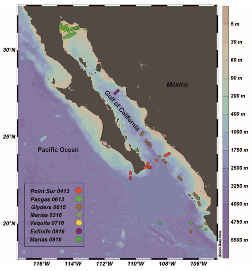
Figure 1.
Map showing the locations of the stations used in this study.

Table 1.
Number of stations from which data for each variable were obtained.
The digital images were captured on an iPad Air 2 with an 8 megapixel camera (San Diego, CA, USA). The Spyglass application [57] was downloaded on this device to determine the tilt angle of the camera and capture the images. The locations of stations were determined by integrating a Bad Elf GPS with the device.
The images were captured following the protocol of Deschamps et al. [58] on days with nil or little cloud cover (maximum 30% coverage allowed) and at a time of the day when the sun was more than 45° above the horizon (between 10:00 am and 4:00 pm for mid-latitudes). To minimize residual polarization and quantify the emerging radiance of water, the observer applied the following steps [58,59]:
- Position his/her body at the bow of the vessel with the sun on his/her back (the sun must be at an angle greater than or equal to 45° relative to the horizon). It is recommended to be located at the bow of the vessel because it is the narrowest and least shady area Figure 2a;
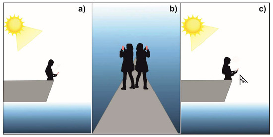 Figure 2. Scheme depicting the steps to follow to capture an image of the sea surface. With the sun on the back (a), rotate 45° to the left or right of the initial position to achieve 135° in the azimuth between the position of the sun and his/her visual field (b), place the camera lens at 45° relative to the sea surface and capture the image (c).
 - Rotate the body 45° to the right or left of the starting position and select a position where the shadow of the vessel is not projected upon the photographic field. According to the methodology proposed by Deschamps et al. [58], this position is required because the observer must be positioned at 135° in the azimuth between the position of the sun and his/her visual field to facilitate measurements from any platform in the ocean, including moving vessels Figure 2b;
- Place the camera at 45°relative to the sea surface, and capture the image Figure 2c.
At least six digital images were captured at each station. We selected images captured at exactly 45° from the sea surface and with no foam within the central zone. To obtain the digital colors (R, G, B), the images were processed in Corel Photo Paint X8. According to Leeuw and Boss [51], for each image, four 1 cm × 1 cm quadrants were selected; in each quadrant, a color histogram was obtained, from which the digital values (R, G, B) were extracted Figure 3. To reduce the natural variability of water color, the digital values of each station were taken as the mean of the values obtained from all quadrants in all the images selected for each station.
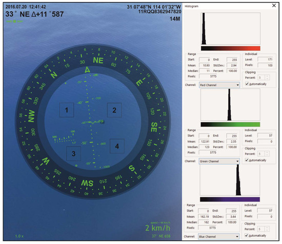
Figure 3.
Example of digital photo processing. The four quadrants selected and the histograms used from this image to obtain the average digital values (R, G, B) are shown.
To estimate the Forel–Ule scale for each station, we applied the criteria of Novoa et al. [60], and the digital values (R, G, B) were converted to chromaticity coordinates (x, y, z) according to the definition of the International Commission on Illumination—x+ y + z = 1; therefore, z = 1 − x – y; hence, the coordinate (z) provides no additional information, so only the coordinates (x, y) are used to represent a color in a chromaticity diagram [60,61].
Once the chromaticity coordinates (x, y) for each image were obtained, they were contrasted with the coordinates estimated by Novoa et al. [60] for each type of Forel–Ule water Table 2. This was carried out by applying the least-squares criteria based on a goodness-of-fit test [62,63].
Table 2.
Chromaticity coordinates (x, y) estimated by Novoa et al. [60] for each Forel–Ule water type.
Measurements of were carried out simultaneously when capturing images of the sea surface. A 30 cm diameter oceanographic disk was used for measurements, which was lowered into the water column from the sunny side of the vessel [26]. The depth at which the disk disappeared from the observer’s view (to the naked eye) was recorded as [30,64]. The Ed (PAR) measurements were conducted with a Li-Cor scalar irradiometer (LI-193) (Lincoln, NE, USA), which recorded the light at 1 m intervals across the water column up to a maximum depth of 30 m.
Subsequently, Kd was estimated based on two methodologies. In the first methodology, it was calculated indirectly from the measurements of and by applying the criteria of Castillo-Ramirez et al. [56]. In the second methodology, the measurements of Ed (PAR) were used based on the criteria of Kirk [27], as expressed in the following equation (Equation (1)):
where Kd is the slope of a linear regression, and the dependent variable is the natural logarithm of irradiance as a function of depth.
Likewise, the oceanographic cruises collected water samples to estimate a(λ) based on the criteria of Mitchell et al. [65] and the concentration of Chla following the methodology of Thomas [66]. a(λ) was estimated considering the light absorption of pure water (aw(λ)), phytoplankton (aphy(λ)), and CDOM ((aCDOM (λ)) [67] (Equation (2)).
The estimated a(λ) was used to classify the stations according to the Jerlov optical water types following the criteria of Solonenko and Mobley [67] and Castillo-Ramirez et al. [56].
The database described above covers a range of optical conditions, from clear (oceanic) to turbid (coastal) waters (Figure 1). For this reason, three types of empirical approaches were generated for each optical variable (Forel–Ule scale, ZSD, Kd, Jerlov scale, and Chla): a general approach that can be applied under oceanic and coastal conditions and two specific approaches to be applied separately under these conditions (oceanic and coastal approaches) Figure 4. The full database, including oceanic and coastal waters, was used for the general approach. For the oceanic and coastal approaches, the stations were classified first by the Jerlov scale Figure 4.
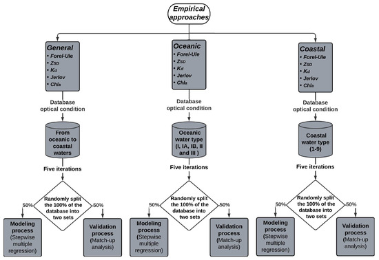
Figure 4.
Scheme of approaches for each optical parameter and the database used for its development.
The empirical approach relates the Forel–Ule scale, ZSD, Kd, the Jerlov scale, and Chla with the digital values (R, G, B) based on a stepwise multiple regression analysis following the Bass criteria [68] (Equation (3)).
where is the variable to predict, which can be the Forel–Ule scale, , , Jerlov scale, a (dependent variable), with (R, G, B) as the independent variables and as their associated coefficients.
On the other hand, to eliminate unusual observations, an analysis of residuals was applied based on the following equation (Equation (4)):
where is the residual; it can be considered as the error calculated as the distance divided by the observed value ( and the modeled value (. Residuals closer to zero indicate a better model performance.
To identify high-noise observations, the criteria of the Six Sigma analysis were followed based on standardized errors [64], where e (Ze) is standardized (Equation (5)).
where is the average of the residuals, and is the standard deviation of the residual.
Once the high-noise observations were removed, the database for each variable was randomly split into two sets: 50% for modeling and 50% for validating purposes [69,70]. To reduce the random error in the selection of the two datasets and test the robustness of the models, we performed five iterations by randomly selecting five different datasets to model, with their respective validation set (Figure 4). A stepwise multiple regression was applied to the data used for modeling, following the criteria of Bass [68].
Subsequently, to demonstrate that the independent variables were significant in each model, a t-test (Equation (6)) was applied to the coefficients associated with each of these variables.
where is the regression coefficient associated with the independent variable, and is the standard error of the coefficient () expressed in the following equations (Equation (7)–(9)):
where (R, G, B) are the digital colors (independent variables).
To test the general significance of the resulting models, an F-test was run based on Equation (10):
where is the number of independent variables (three in this case), is the squared mean of the regression, and is the squared mean of the residual error.
The proportion of the variation of the dependent variable that can be explained by independent variables was estimated with the coefficient of determination () (Equation (11)).
where is the variability explained by the model, and is the variability explained by .
Once the models for each variable were obtained, they were validated based on a match-up analysis [71], where the statistical validity of the models was estimated using the Pearson correlation coefficient (rP), expressed as (Equation (12)):
where rP is the Pearson correlation, Covmodel,val is the covariance of the modeled and validated datasets, and SDmodel and SDval are the standard deviations of the modeled and validated datasets, respectively. This coefficient is a measure of the linear correlation between two variables; it ranges between −1 and +1 (where +1 indicates a direct linear relationship, −1 indicates an inverse linear relationship, and 0 indicates a nonlinear relationship).
In order to compare the models estimated in this work with those from the literature, three statistical descriptors were calculated: mean absolute error () (Equation (13)), root-mean square error () (Equation (14)), and analysis of bias (BIAS) (Equation (15)).
where n is the total number of data points included in this analysis, represents residual observations, and is the absolute value of residuals.
where BIAS is the residual mean.
Lower and values represent better results, whereas BIAS values closer to zero indicate better results. To determine which was the best model, the model performance index (MPI) was estimated [56] (Equation (16)), which is based on the three statistical descriptors mentioned above.
where are the range of and , respectively; is the absolute range of ; and p is the total number of compared models. The ranks were calculated following the criteria of Wilcoxon [72]. The MPI intervals range from 0 to 1, where values closer to 1 represent a better model.
To evaluate whether the differences between the in situ values and the results obtained from the 45° and non-45° images were statistically significant, the models mentioned above were applied for those stations that met the following criteria: (1) stations that had in situ data for the variable to be modeled, (2) R, G, B values obtained from images captured at 45°, and (3) R, G, B values obtained from images captured at an angle other than 45°. Following in situ quality control, whereby only images captured at or close to a 45° angle were retained, these data only included images captured with a ± 1° difference (44° and 46°). A non-parametric ANOVA analysis was performed by Friedman blocks following the criteria of Friedman [73] (Equation (17)).
where r is the number of observations, k is the number of treatments, and is the sum of the ranges in each treatment.
Once the differences were analyzed and to determine which results presented the lowest error, a standardized residual analysis was run (Equation (5)). Values closer to zero indicates a lower error.
To estimate the accuracy of the results, a confidence interval was established based on tcrít α/2, n−1 with an α of 95%; then, we calculated the percentage of the data that were within this interval. Finally, the data accuracy was tested based on a least-square test applied to the residuals following the criteria of Xu et al. [62]; the most accurate data are those with the lowest X2 value.
3. Results and Discussion
The approaches proposed in this work are empirical; therefore, they depend on the boundary limits established by the variables used in their development [26,74]. Empirical modeling of ocean color and optical parameters is challenged by limited sampling opportunity on sunny days with calm seas. These conditions are essential to obtain data that represent the true variability of the light field in water [75,76,77]. To address this challenge, in this research, we used data from seven oceanographic cruises carried out between 2013 and 2016. In each cruise, a sampling network of more than 70 stations was established. However, data could only be obtained at approximately 15% of the established stations due to unfavorable conditions (e.g., cloudy days and waves) Table 1. In addition, it is necessary to obtain an independent dataset to validate the developed model. This validation is essential to assess the ability of the model to predict values [26,74].
To address these challenges, the database for each variable was divided into two independent groups, using 50% of the data for the modeling process and the other 50% for validation. In addition, to ensure the robustness of the models, five iterations were performed randomly, selecting five different datasets to model, each with its corresponding validation set [56,69,70] (Figure 4). This approach helped to reduce the random error associated with the selection of the two datasets.
3.1. General Approach
The general approach was estimated from the complete database with optical conditions ranging from oceanic to coastal. This showed that the non-significant independent variable for the estimation of most parameters was the digital color R corresponding to the red wavelength (700 nm) Table 3. This is because the light absorption by water increases exponentially toward the red region of the electromagnetic spectrum [78], which implies a lower penetration capacity into the water column, a lower reflection of long wavelengths (~700 nm), and, therefore, fewer possibilities to react to changes in optically active compounds [27,79]. The only case in which the three digital colors (R, G, B) were significant Table 3 was to estimate the Forel–Ule scale (Equation (18)). This result may have occurred because this scale, unlike the parameters used in the other approaches, is based on a visual perception of water color, which results from the combination of these three colors (R, G, B) [80].
Table 3.
Results of the stepwise multiple regression analysis of the models for the general approach (.
Once the significant variables were identified, we confirmed that the general approach for all the parameters (Equations (18)–(22)) was significant (Table 3, column 10 (>)). This finding implies that the partition of a digital image into digital channels (R, G, B) and the association of these channels with in situ data of surface optical parameters can be also used to estimate ZSD, Kd, and the Jerlov scale. In addition, these findings support the reports by Goddijn-Murphy et al. [48], Novoa et al. [50], and Leeuw and Boss [51], who suggested the use of images as an alternative to estimate Chla, turbidity, and the Forel–Ule scale.
Subsequently, this approach was validated based on the criteria proposed by Gregg and Casey [81], Djavidnia et al. [82], and Santamaría-del-Ángel et al. [71], who established that rpcal values above 0.70 indicate a strong association. These criteria suggest that the correlations between the modeled and validation data were mostly highly significant Table 4. The Kd model expressed by (Equation (20)) yielded the lowest values. To improve Kd estimation, the criteria of Castillo-Ramirez et al. [56] were used based on values modeled according to (Equation (19)). The Castillo-Ramirez et al. [56] criteria yielded higher correlation values (= 0.85) Table 4; therefore, we propose this as the best alternative for estimating Kd from a digital image.
Table 4.
Results of the validation analysis of the models for the general approach.
3.2. Oceanic and Coastal Approaches
Morel and Prieur [34] proposed the classification of seawater into two types: case 1 and optically complex waters. Case 1 waters are those whose optical properties are driven mainly by phytoplankton and are generally found in oceanic areas far from the continental shelf. Optically complex waters contain suspended sediments, non-phytoplanktonic organic particles, or CDOM, in addition to phytoplankton. The sources of these compounds are frequently associated with coastal areas; however, in some cases, it is also possible to observe optically complex waters in oceanic areas. For instance, a phytoplanktonic bloom would increase CDOM levels in an oceanic water plot and would provide it with optically complex characteristics [34,79,83].
The approaches for oceanic and coastal conditions were obtained to assess whether more specific models (in terms of optical conditions) are more accurate to estimate the studied parameters. The results of the oceanic approach Table 5 show that none of the three digital colors (R, G, B) was significant for most of the parameters. The only significant model for the oceanic approach was that for the estimation of the Forel–Ule scale (Table 5; Equation (23)). The greatest quantity of optical components that produce a change in water color occurs in coastal areas, where they have a high variability [34]. The results obtained in the present work Table 5 indicate that water color changes in oceanic regions are not significant enough to be captured in a digital image to be associated with ZSD, Kd, the Jerlov scale, and Chla.
Table 5.
Results of stepwise multiple regression analysis for the oceanic approach models (.
The coastal approach showed that the digital color G was significant in all models, for some parameters in combination with the digital colors R or B Table 6. This variation in significant digital colors (or wavelengths) depends on the nature and quantity of particles present in the studied water plot [25]. Specifically:
Table 6.
Results of the stepwise multiple regression analysis for the coastal approach models (.
- Phytoplankton produces a green coloration in the water when it is in high concentrations due to the presence of Chla in cells, except for certain species that produce a red or brown coloration;
- Non-phytoplankton material (or detritus) produces a brown or reddish coloration depending on the source of the material;
- CDOM stains water a yellow–brown color.
The coastal approach was significant to estimate all the variables (Equations (24)–(28)) Table 6, the Forel–Ule scale, the Jerlov scale, ZSD, Kd, and Chla under optically complex conditions. The degree of association between modeled and validation data (rPcal) for the oceanic and coastal approach Table 7 was higher than that obtained in the general approach Table 4. The validation of these models shows that a more specific approach in terms of optical conditions results in greater accuracy Table 7. The model that yielded lower values than those reported for the general approach was that predicting the Jerlov scale (Equation (27)). This may be because the model proposed by Solonenko and Mobley [67] for associating a(λ) with the Jerlov water type ignores the contribution of non-phytoplanktonic particulate matter. This component includes phytoplankton, detritus, and other organic particles and minerals (Equation (2)), which represent important contributions in coastal areas, as reported by Morel and Prieur [34].
Table 7.
Results of the model validation analysis for the oceanic and coastal approaches.
3.3. Model Comparison
Table 8 shows a comparison of the performance of our general and coastal models (Equations (22) and (28)) with models proposed by Goddijn-Murphy et al. [48]. These authors developed two models, in which the B/G ratios are the independent variables and is the dependent variable.
Table 8.
general and coastal models compared with literature models.
The results presented in Table 8 show that the models proposed in this work achieved a better performance in the validation process compared to those reported in the literature applied to our data, demonstrating the relevance of acquiring field data under appropriate conditions (e.g., sunny days and calm sea). These conditions were not observed by Goddijn-Murphy et al. [48]. Additionally, the lower R2 obtained by Goddijn-Murphy et al. [48] could be due to the high CDOM concentrations reported, which could affect the absorption of blue wavelengths in water.
Gao et al. [53] developed an algorithm to estimate using smartphone images in continental water bodies. These authors observed the same conditions as in our study, including camera and sun angles. However, we could not apply their model to our data because it was developed for other conditions. Continental waters with high CDOM concentrations are characterized by high reflectance in R and high absorption in B [48]. They also used a limnologic Secchi disk, while in this research, an oceanic disk was used. Differences in terms of size and reflectance surface are noticeable in both versions [26,56], so they are not comparable.
3.4. Angle Effect
Friedman’s non-parametric analysis showed significant differences between the ZSD (Equation (25)) and the Chla (Equation (28)) values obtained from an image captured at 45° and at an angle other than 45° Table 9.
Table 9.
Results of the non-parametric Friedman analysis (α = 0.05), where = .
Subsequently, the precision of the results was evaluated; to this end, a confidence interval of ±2.08 was set when using the model to predict ZSD (Equation (25)) and ±2.06 for Chla (Equation (28)) Figure 5a,b. This methodology showed that when applying the ZSD model (Equation (25)), 95.45% of the data obtained from 45° images were within the confidence interval, while only 86.36% were within this interval for non-45° images Figure 5a. It was also observed that the data outside the confidence interval were underestimated. On the other hand, when we applied the Chla model (Equation (28)), 95.45% of the 45° data and 90.90% of non-45° data fell within the confidence interval Figure 5b. In this case, the data outside the interval are overestimated. Once the differences and precision of the results were analyzed, their accuracy was evaluated; the lowest X 2 values correspond to the results obtained using 45° images Table 10. This finding indicates that these results, in addition to being more precise, are more accurate.
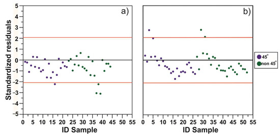
Figure 5.
Analysis of standardized residuals. (a) model; (b) Chla model.
Table 10.
Least-squares analysis for the and and Chla models.
4. Discussion
The methods traditionally used for in situ monitoring to estimate optical parameters involve the use of specialized instrumentation, which can be relatively complex and expensive [63,66,67,84,85,86,87,88,89,90]. In addition, these methods involve a slow analytical process, making them ineffective to obtain a large-scale view of the study area in a short time [48,90]. On the other hand, the logistics involved in preparing in situ monitoring based on optical parameters is not straightforward; it requires a vessel, field material, and personnel experienced in recording measurements and collecting samples. These monitoring procedures should be scheduled on sunny days, as clouds can distort light measurements in the water during field work [75,76,77].
- The results of this study show the potential of digital images to evaluate the surface optical parameters of a water plot. The main advantage of the proposed approaches is their easy implementation and low cost, since they do not demand optics expertise and only require a digital camera. These advantages can be summarized as follows [47,48,49,50,51,52,53,54,91,92,93,94,95,96]:
- Low-cost system: The use of smartphones, tablets, or digital cameras to capture digital images is a cost-effective method for estimating surface optical parameters in the ocean, as it does not require expensive specialized equipment. Smartphones and other devices are relatively inexpensive and widely available, making them an attractive option for researchers who are working with limited budgets or who do not have access to specialized instrumentation;
- Accessibility and ease of use: since these electronic devices are widely used, this methodology can provide a widespread network of data acquisition, which can be essential for global-scale analyses and modeling;
- High spatial and temporal resolution: digital image capture can provide high spatial and temporal resolution, allowing for a more detailed analysis of the ocean’s surface optical properties over a larger area;
- Versatility: smartphones, tablets, or digital cameras can be used to capture images from different platforms such as beaches, piers, and boats, making them versatile tools for surface optical parameter estimation;
- Citizen science: The use of digital images allows for citizen scientists to contribute to the data acquisition process. This can increase public participation in scientific research and environmental monitoring, as well as their awareness and engagement in oceanographic research;
- Environmental monitoring: Surface optical parameters play a crucial role in the health of marine ecosystems. The use of electronic devices can aid in environmental monitoring efforts, providing critical information for decision-making and conservation efforts;
- Rapid response: in the event of a phytoplankton bloom, the use of digital images can aid in rapid response efforts, providing real-time information on the extent and severity of spills.
This type of low-cost, user-friendly approach not only benefits scientists but could also be used by the tourism or aquaculture industries, as well as by individual citizens concerned about changes in the water quality in their local environment. The benefits of this approach go beyond just improving data collection. By enabling real-time and continuous monitoring of surface optical parameters, this approach provides valuable information for environmental management and decision making. The enhanced resolution and coverage of the data also offers new opportunities for researchers to investigate the complex relationships between surface optical parameters and environmental processes. This is especially important in coastal areas, where our results are more accurate, since 355 million people are expected to live within the 100 km of the coast between 2020 and 2035 [16,97,98]. This continuously increasing pressure will likely lead to the degradation of these ecosystems, adversely impacting the provided ES [26,99]. We propose implementing the use of the coastal approach to supplement traditionally used analyses for in situ monitoring.
Taking into account these advantages, using the model generated for the Jerlov scale (Equation (27)), as an example, would help to classify water types in a quick and efficient way, since the equipment currently used to define water types based on this scale require specialized knowledge for their use. This is the case of hyperspectral irradiometers [87] or spectrophotometers (for calculating inherent optical properties) if the criteria of Solonenko and Mobley [67] are followed, as in the cruises used to build the database used in the present study. Likewise, approaches such as that proposed by Mallick et al. [89], where Kd values are derived from satellite images, may be considered for estimating the Jerlov scale. However, as mentioned by Lebourgeois et al. [47], the processing of such images is more complex relative to digital images. In turn, the approach proposed herein could be used to obtain and monitor optical properties such as , the total dispersion coefficient (), and Kd , since, as reported by Jerlov [33] and Solonenko and Mobley [67], each Jerlov water type is associated with a typical spectrum of these properties. Therefore, a shift in the Jerlov water type may indicate that the components in the water column (phytoplankton, detritus, and CDOM) and the light field are changing.
Estimating Chla concentrations with the model proposed in this work (Equation (28)) would help us to monitor phytoplankton blooms [100,101] at a lower cost and more quickly. This is because the methodologies currently used in laboratories involve equipment such as spectrophotometers or high-performance liquid chromatography (HPLC), which require a filtration system, fiberglass filters, and solvents [66,102]. In addition, the methodology involving HPLC also requires standards of pigments to estimate their concentration and takes approximately 48 h [66]. However, phytoplankton blooms are proliferation events that can last less than 24 h (fast blooms), for several days, or for weeks [103]. Therefore, a rapid response can be crucial.
The estimated models to predict ZSD (Equation (25)) and water color based on the Forel–Ule scale (Equations (23) and (24)) could be used to monitor eutrophication and anoxic–hypoxic events, which influence water color and transparency [104,105,106]. In addition, they would assist us to obtain data on these variables on sunny days when a Secchi disk or color comparators are unavailable. In addition, in the case of the Forel–Ule scale, this approach allows for estimation of all 21 colors of the scale, as the currently used instrument only shows 16 color comparators.
Thus, this approach may facilitate surveying the water status in the study area without the need to collect water samples or previous planning. For example, data could be obtained on sunny days when no field trips are scheduled. However, it is worth noting that the reliability and usefulness of this approach requires additional in situ measurements to carry out additional calibration and validation studies.
In addition, the algorithms proposed herein may be implemented in the development of an app that provides the Forel–Ule scale, ZSD, Kd, the Jerlov scale, and Chla. However, to obtain high-quality data, it would be essential to implement quality flags such as those used in the “Eye on water” app 2.4.0 [107], where the user is asked to perform a test prior to capturing the image.
Although the use of digital images to estimate surface optical parameters in the ocean has notable advantages in terms of ease of use and low cost, it is important to mention that there are limitations that must be considered. One issue that could arise is whether different technologies used in smartphone cameras could generate different RGB readings. However, Leeuw and Boss [51] evaluated the spectral sensitivity of RGB channels in different next-generation devices and showed that although there may be differences in the spectral shape, the values in RGB peaks are practically the same between devices. The approaches presented in this work are based on the RGB peaks Figure 3, so they should be valid regardless of the device being used. Another issue is the interpretation of color changes in a relatively small area (1 cm × 1 cm). Our methodology is based on the work of Leeuw and Boss [51], who proposed establishing a fixed area within the photograph so that devices with cameras of different resolutions can be compared with each other, thanks to the fact that the field of view of the camera is the same between devices.
Variability in lighting and image quality can be critical factors that influence the quality of the obtained data, as mentioned in [75,76,77]. The quantity and quality of light reaching the ocean surface depends mainly on the position of the sun and cloud cover [27,28]. The image quality can be affected by elements influencing the visual state of the ocean surface, for example, the presence of waves or white caps, sunshine, or the shadows generated by the boat or platform from which the image is captured [50,51,53,58,59].
To overcome these limitations and obtain quality data, we followed the reflectance measurement methodology with a SIMBAD spectroradiometer to capture the photographs (refer to [58]). As mentioned by Fougnie et al. [108] and Deschamps et al. [58], this methodology is very specific with respect to the sun position and angle, as well as the equipment angles, and it allows for a reduction in the noise or interference caused by the sunshine and the reflection of the sky on the water surface. Digital images were captured at an angle of 45° relative to the ocean surface on sunny days, when the sun was at an angle equal to or greater than 45° relative to the horizon and with little or no cloud cover. A 45° sun position at the zenith minimizes Fresnel reflectance on the water surface, allowing greater light penetration, improving the accuracy of radiometric measurements, and facilitating accurate estimation of optical parameters in the ocean [108].
5. Conclusions
Changes in color or turbidity in the marine environment involve an alteration of the components that absorb or disperse light within the water column. These changes can be associated with natural or anthropogenic processes that affect water quality, such as anoxia–hypoxia, eutrophication, and phytoplanktonic blooms. Therefore, it is advisable to implement monitoring systems to generate time series with a sufficient time span to differentiate between natural variabilities and those derived from anthropogenic pressures.
A simple way to carry out this sort of monitoring without incurring high costs is to apply techniques such as the one proposed in the present work, which only require a smartphone or tablet. The results of this study demonstrate that images captured at the sea surface with the methodology described herein provide information about the optical characteristics (such as the Forel–Ule scale, ZSD, Kd, the Jerlov scale, and Chla) of a water plot. The use of these images for the development of empirical approaches yielded the best results in the coastal area. In addition, this study confirmed that if the established methodology for image capture is not followed in relation to the camera positioning angle, the results can be biased by the noise generated by the solar brightness and the reflection of the sky on the water surface. The conditions required for the proper performance of our approach that the image of the water surface be captured on days with low or no cloud cover, with a calm sea, and when the sun is behind the observer at an angle greater than or equal to 45° with respect to the horizon. Once the above conditions are met, the observer must turn his/her body 45° to the right or left of the starting position and select a position where the shadow of the boat does not interfere in the image recording field. Finally, the camera should be positioned at 45° relative to the sea surface to capture the image.
This user-friendly and low-cost methodology could be used as a supplement to the analyses traditionally applied in in situ monitoring. The observer does not necessarily have to be an expert in optics to use it, which facilitates its implementation in monitoring schemes involving citizen assistance for data generation. This advantage would help to expand the spatiotemporal coverage of monitoring. However, it is worth noting that the reliability and usefulness of this approach must be supplemented by in situ measurements to carry out additional calibration and validation studies. Moreover, this work establishes a basis for the future development of an app to deliver the Forel–Ule scale, ZSD, Kd, the Jerlov scale, and Chla, which could be suitable for use by scientists and the general public. To obtain data reflecting the true variability of a water plot and filter out images that fail to meet the methodological criteria, this app should include quality flags considering the angles of the observer and the camera relative to the position of the sun. In addition, this app should record information including the date, time, global position, and distance from the water surface. The above can be achieved with the tools currently included in mobile devices, such as calendar, clock, global positioning system (GPS), and barometer. For free access to the data, we also recommend developing a web page where these data can be viewed in real time and downloaded.
Author Contributions
Conceptualization, A.C.-R., E.S.-d.-Á., A.G.-S., J.A.-M., J.L.-C. and M.-T.S.-F.; methodology, A.C.-R., E.S.-d.-Á. and M.-T.S.-F.; software, A.C.-R., E.S.-d.-Á., M.-T.S.-F. and J.A.-M.; validation, A.C.-R., E.S.-d.-Á., M.-T.S.-F., J.A.-M. and J.L.-C.; formal analysis, A.C.-R., E.S.-d.-Á., A.G.-S., J.A.-M., J.L.-C. and M.-T.S.-F.; investigation, A.C.-R., E.S.-d.-Á., A.G.-S., J.A.-M., J.L.-C. and M.-T.S.-F.; resources, E.S.-d.-Á., A.G.-S., J.L.-C. and M.-T.S.-F.; data curation, A.C.-R. and E.S.-d.-Á.; writing—original draft preparation, A.C.-R., E.S.-d.-Á. and M.-T.S.-F.; writing—review and editing, A.C.-R., E.S.-d.-Á., A.G.-S., J.A.-M., J.L.-C. and M.-T.S.-F.; visualization, A.C.-R., E.S.-d.-Á. and M.-T.S.-F.; supervision, A.C.-R., E.S.-d.-Á., A.G.-S., J.A.-M., J.L.-C. and M.-T.S.-F.; project administration, A.C.-R., E.S.-d.-Á., A.G.-S., J.A.-M., J.L.-C. and M.-T.S.-F.; funding acquisition, E.S.-d.-Á., A.G.-S., J.L.-C. and M.-T.S.-F. All authors have read and agreed to the published version of the manuscript.
Funding
This research was funded by the projects "Influencia de remolinos de mesoescala sobre hábitats de larvas de peces (con énfasis en especies de importancia comercial) en la zona de mínimo de oxígeno del océano pacífico frente a México: océano abierto y efecto de islas" (“Influence of Mesoscale Eddies on the Habitats of Fish Larvae (with Emphasis on Species of Commercial Importance) in the Oxygen Minimum Layer of the Pacific Ocean off Mexico: Open Ocean and Effect of Islands”) (SEP-CONACyT 236864), “Fronteras de la Ciencia: Probando paradigmas sobre la expansión de la zona del mínimo de oxígeno: reducción del hábitat vertical del zooplancton y su efecto en el ecosistema pelágico mediante métodos de muestreo autónomos” (“Frontiers of Science: Testing Paradigms on the Expansion of the Oxygen Minimum Layer: Reduction of the Vertical Habitat of Zooplankton and its Effect on the Pelagic Ecosystem through Autonomous Sampling Methods”) (CONACYT 8662), “Flujo atmosférico de metales bioactivos y sus solubilidad en el Golfo de California: un escenario hacia el cambio climático” (“Atmospheric Flow of Bioactive Metals and their Solubility in the Gulf of California: a Scenario toward Climate Change (UABC-IIO), “Regionalización dinámica de la Bahía de Todos Santos mediante imágenes de color del océano” (“Dynamic Regionalization of Todos Santos Bay through Ocean Color Images” supported by the 18th Internal Call at UABC, ANTARES (IAI CRN393), SIMAC-CONACYT; “Dinámica Costera En Inmediaciones De San Felipe, B.C. (“Coastal Dynamics in the Vicinity of San Felipe, B.C.”); “Condiciones Oceanográficas Del Área De Refugio Para La Protección De La Vaquita Marina e Inmediaciones” (“Oceanographic Conditions in the Reserve Area for the Protection of the Vaquita and Adjacent Areas" (Secretariat of the Navy); “Estudio integral para la determinación del polígono para vertimientos de materiales producto del dragado en bahía Sebastián Vizcaíno, B.C.” (“Integral Study to Determine the Polygon for Emptying Dredged Materials in Bahia Sebastian Vizcaino, B.C.”) (Secretariat of the Navy), SIMAC-2000107017 (CICESE); and “Ecological Monitoring of the Upper Gulf of California” (PANGAS-Packard Foundation); INP-CICIMAR: SIP 1721,20160514-CONACYT 236864). M.-T.S.-F. was the beneficiary of two postdoctoral research grants: one from the Spanish Ministry of Education Culture and Sports (number CAS18/00107) and one from the Valencian Conselleria d’Educació, Investigació, Cultura i Esport (number BEST/2017/217)—both in support of her stay at the Universidad Autónoma de Baja California (México) during her advisory time.
Institutional Review Board Statement
Not applicable.
Informed Consent Statement
Not applicable.
Data Availability Statement
Not applicable.
Acknowledgments
The authors wish to thank Consejo Nacional de Ciencia y Tecnología (CONACyT) for the grant awarded to the first author for her studies. The authors also thank the SIMBIOS NASA Program, Universidad Autónoma de Baja California, Instituto de Investigaciones Oceanológicas, Centro de Investigación Científica y de Educación Superior de Ensenada, Secretaría de Marina Armada de México, Dirección General Adjunta de Oceanografía, Hidrografía y Meteorología, Instituto Politécnico Nacional. Maria Elena Sánchez-Salazar translated the manuscript into English.
Conflicts of Interest
The authors declare no conflict of interest.
References
- Santamaría-del-Angel, E.; Sebastia-Frasquet, M.T.; Millán-Nuñez, R.; González-Silvera, A.; Cajal-Medrano, R. Anthropocentric bias in management policies. Are we efficiently monitoring our ecosystem. In Coastal Ecosystems: Experiences and Recommendations for Environmental Monitoring Programs; Sebastiá-Frasquet, M.T., Ed.; Nova Science Publishers: New York, NY, USA, 2015; Chapter 1; pp. 1–12. ISBN 978-1-63482-189-6. [Google Scholar]
- Millennium Ecosystem Assessment (Program). Ecosystems and Human Well-Being: Synthesis; Island Press: Washington, DC, USA, 2005; p. 155. ISBN 1-59-726040-1. [Google Scholar]
- MacDougall, A.S.; McCann, K.S.; Gellner, G.; Turkington, R. Diversity Loss with Persistent Human Disturbance Increases Vulnerability to Ecosystem Collapse. Nature 2013, 494, 86–89. [Google Scholar] [CrossRef] [PubMed]
- Cearreta, A. La Perspectiva Del Antropoceno: Una Mirada Geológica al Cambio Climático. Metode 2021, 12, 107–113. [Google Scholar] [CrossRef]
- Leadley, P.; Pereira, H.M.; Alkemade, R.; Fernandez- Manjarres, J.F.; Proenca, V.; Scharlemann, J.P.W.; Walpole, M.J. Escenarios de biodiversidad: Proyecciones del siglo XXI a los cambios de biodiversidad y sus servicios ecosistémicos. In Serie Técnica Numero 50; Secretaria del Convenio Sobre Diversidad Biológica: Montreal, QC, Canada, 2010; p. 55. [Google Scholar]
- Waters, C.N.; Zalasiewicz, J.; Summerhayes, C.; Barnosky, A.D.; Poirier, C.; Gałuszka, A.; Cearreta, A.; Edgeworth, M.; Ellis, E.C.; Ellis, M.; et al. The Anthropocene Is Functionally and Stratigraphically Distinct from the Holocene. Science 2016, 351, aad2622. [Google Scholar] [CrossRef] [PubMed]
- Sebastiá-Frasquet, M.T. Coastal Ecosystems: Experiences and Recommendations for Environmental Monitoring Programs; Nova Science Publishers: New York, NY, USA, 2015; p. 228. ISBN 978-1-63482-189-6. [Google Scholar]
- Kitsiou, D.; Karydis, M. Marine Spatial Planning: Methodologies, Environmental Issues and Current Trends; Nova Science Publishers: New York, NY, USA, 2017; p. 491. ISBN 978-1-53612-170-4. [Google Scholar]
- ANTARES: Latin America. NANO | NF-POGO Alumni Network for the Ocean. Available online: https://nf-pogo-alumni.org/projects/latin-america/ (accessed on 7 October 2020).
- HOT: The Hawaii Ocean Time-Series. Available online: https://hahana.soest.hawaii.edu/hot/ (accessed on 7 October 2020).
- California Current Ecosystem LTER. Available online: https://lternet.edu/site/california-current-ecosystem-lter/ (accessed on 7 October 2020).
- Ceccaroni, L.; Piera, J.; Wernand, M.R.; Zielinski, O.; Busch, J.A.; Van Der Woerd, H.J.; Bardaji, R.; Friedrichs, A.; Novoa, S.; Thijsse, P.; et al. Citclops: A next-Generation Sensor System for the Monitoring of Natural Waters and a Citizens’ Observatory for the Assessment of Ecosystems’ Status. PLoS ONE 2020, 15, e0230084. [Google Scholar] [CrossRef]
- OED Oxford English Dictionary. Available online: https://www.oed.com/start?showLogin=false (accessed on 12 June 2019).
- Bøgestrand, J.; Kristensen, P.; Kronvang, B. Source Apportionment of Nitrogen and Phosphorus Inputs into the Aquatic Environment; European Environment Agency: Copenhagen, Denmark, 2005; p. 48. ISBN 9-29-167777-9. [Google Scholar]
- Jovanovic, S.; Carrion, D.; Brovelli, M.A. Citizen science for water quality monitoring applying foss. Int. Arch. Photogramm. Remote Sens. Spat. Inf. Sci. 2019, XLII-4/W14, 119–126. [Google Scholar] [CrossRef]
- Shukla, P.R.; Skea, J.; Calvo Buendia, E.; Masson-Delmotte, V.; Pörtner, H.-O.; Roberts, D.C.; Zhai, P.; Slade, R.; Connors, S.; van Diemen, R.; et al. Climate Change and Land: An IPCC Special Report on Climate Change, Desertification, Land Degradation, Sustainable Land Management, Food Security, and Greenhouse Gas Fluxes in Terrestrial Ecosystems; Intergovernmental Panel on Climate Change (IPCC): Geneva, Switzerland, 2019. [Google Scholar]
- Buonocore, E.; Grande, U.; Franzese, P.P.; Russo, G.F. Trends and Evolution in the Concept of Marine Ecosystem Services: An Overview. Water 2021, 13, 2060. [Google Scholar] [CrossRef]
- Amaral, V.; Romera-Castillo, C.; García-Delgado, M.; Gómez-Parra, A.; Forja, J. Distribution of Dissolved Organic Matter in Estuaries of the Southern Iberian Atlantic Basin: Sources, Behavior and Export to the Coastal Zone. Mar. Chem. 2020, 226, 103857. [Google Scholar] [CrossRef]
- Oh, Y.H.; Kim, Y.; Park, S.R.; Lee, T.; Son, Y.B.; Park, S.-E.; Lee, W.C.; Im, D.-H.; Kim, T.-H. Spatiotemporal Change in Coastal Waters Caused by Land-Based Fish Farm Wastewater-Borne Nutrients: Results from Jeju Island, Korea. Mar. Pollut. Bull. 2021, 170, 112632. [Google Scholar] [CrossRef]
- Kratzer, S.; Kyryliuk, D.; Brockmann, C. Inorganic Suspended Matter as an Indicator of Terrestrial Influence in Baltic Sea Coastal Areas—Algorithm Development and Validation, and Ecological Relevance. Remote Sens. Environ. 2020, 237, 111609. [Google Scholar] [CrossRef]
- Li, P.; Ke, Y.; Wang, D.; Ji, H.; Chen, S.; Chen, M.; Lyu, M.; Zhou, D. Human Impact on Suspended Particulate Matter in the Yellow River Estuary, China: Evidence from Remote Sensing Data Fusion Using an Improved Spatiotemporal Fusion Method. Sci. Total Environ. 2021, 750, 141612. [Google Scholar] [CrossRef]
- Guo, F.; Jiang, G.; Liu, F. Plankton Distribution Patterns and the Indicative Significance of Diverse Cave Wetlands in Subtropical Karst Basin. Front. Environ. Sci. 2022, 10, 1409. [Google Scholar] [CrossRef]
- Bharathi, M.D.; Sarma, V.V.S.S.; Ramaneswari, K.; Venkataramana, V. Influence of River Discharge on Abundance and Composition of Phytoplankton in the Western Coastal Bay of Bengal during Peak Discharge Period. Mar. Pollut. Bull 2018, 133, 671–683. [Google Scholar] [CrossRef]
- Kvesić, M.; Vojković, M.; Kekez, T.; Maravić, A.; Andričević, R. Spatial and Temporal Vertical Distribution of Chlorophyll in Relation to Submarine Wastewater Effluent Discharges. Water 2021, 13, 2016. [Google Scholar] [CrossRef]
- Prieur, L.; Sathyendranath, S. An Optical Classification of Coastal and Oceanic Waters Based on the Specific Spectral Absorption Curves of Phytoplankton Pigments, Dissolved Organic Matter, and Other Particulate Materials. Limnol. Oceanogr. 1981, 26, 671–689. [Google Scholar] [CrossRef]
- Santamaría-del-Angel, E.; Soto, I.; Millán-Nuñez, R.; González, A.; Wolny, J.; Cerdeira-Estrada, S.; Cajal-Medrano, R.; Muller, F.; Padilla-Rosas, Y.X.S.; Mercado-Santana, A.; et al. Phytoplankton Blooms: New Initiative Using Marine Optics as a Basis for Monitoring Programs. In Coastal Ecosystems: Experiences and Recommendations for Environmental Monitoring Programs; Sebastiá-Frasquet, M.T., Ed.; Nova Science Publishers: New York, NY, USA, 2015; Chapter 4; pp. 57–88. ISBN 978-1-63482-189-6. [Google Scholar]
- Kirk, J.T. Light and Photosynthesis in Aquatic Ecosystems, 2nd ed.; Cambridge University Press: Cambridge, UK, 2011; p. 649. [Google Scholar]
- Mobley, C.D. Light and Water: Radiative Transfer in Natural Waters; Academic Press: New York, NY, USA, 1994; p. 565. [Google Scholar]
- Arnone, R.A.; Wood, A.M.; Gould, R.W. The evolution of optical water mass classification. Oceanogr 2004, 17, 14–15. [Google Scholar] [CrossRef]
- Secchi, A. Schreiben Des Herrn Prof. Secchi, Directors Der Sternwarte Des Collegio Romano, an Den Herausgeber. Astron. Nachr. 1866, 68, 63. [Google Scholar] [CrossRef]
- Ule, W. Die Bestimmung der Wasserfarbe in Den Seen. Kleinere Mittheilungen. Dr. A. Petermanns Mittheilungen Aus Justus Perthes Geographischer Anstalt; Justus Perthes: Gotha, Germany, 1892; pp. 70–71. [Google Scholar]
- Forel, F. Couleur de L’Eau in Optique, Le Léman. Monographie Limnologique, 2nd ed.; Slatkins: Geneve, Switzerland, 1895; p. 538. [Google Scholar]
- Jerlov, N.G. Optical Studies of Ocean Water. Rept. Swedish Deep-Sea Exped. 1951, 3, 1–59. [Google Scholar]
- Morel, A.; Prieur, L. Analysis of Variations in Ocean Color. Limn. Oceanogr. 1977, 22, 709–722. [Google Scholar] [CrossRef]
- Moore, T.S.; Campbell, J.W.; Dowell, M.D. A Class-Based Approach to Characterizing and Mapping the Uncertainty of the MODIS Ocean Chlorophyll Product. Remote Sens. Environ. 2009, 113, 2424–2430. [Google Scholar] [CrossRef]
- Lubac, B.; Loisel, H. Variability and Classification of Remote Sensing Reflectance Spectra in the Eastern English Channel and Southern North Sea. Remote Sens. Environ. 2007, 110, 45–58. [Google Scholar] [CrossRef]
- Mélin, F.; Zibordi, G.; Berthon, J.-F.; Bailey, S.; Franz, B.; Voss, K.; Flora, S.; Grant, M. Assessment of MERIS Reflectance Data as Processed with SeaDAS over the European Seas. Opt. Express 2011, 19, 25657–25671. [Google Scholar] [CrossRef] [PubMed]
- Tilstone, G.H.; Peters, S.W.M.; van der Woerd, H.J.; Eleveld, M.A.; Ruddick, K.; Schönfeld, W.; Krasemann, H.; Martinez-Vicente, V.; Blondeau-Patissier, D.; Röttgers, R.; et al. Variability in Specific-Absorption Properties and Their Use in a Semi-Analytical Ocean Colour Algorithm for MERIS in North Sea and Western English Channel Coastal Waters. Remote Sens. Environ. 2012, 118, 320–338. [Google Scholar] [CrossRef]
- Vantrepotte, V.; Loisel, H.; Dessailly, D.; Mériaux, X. Optical Classification of Contrasted Coastal Waters. Remote Sens. Environ. 2012, 123, 306–323. [Google Scholar] [CrossRef]
- Moore, T.S.; Dowell, M.D.; Bradt, S.; Ruiz Verdu, A. An Optical Water Type Framework for Selecting and Blending Retrievals from Bio-Optical Algorithms in Lakes and Coastal Waters. Remote Sens. Environ. 2014, 143, 97–111. [Google Scholar] [CrossRef] [PubMed]
- Mélin, F.; Vantrepotte, V. How Optically Diverse Is the Coastal Ocean? Remote Sens. Environ. 2015, 160, 235–251. [Google Scholar] [CrossRef]
- Ye, H.; Li, J.; Li, T.; Shen, Q.; Zhu, J.; Wang, X.; Zhang, F.; Zhang, J.; Zhang, B. Spectral Classification of the Yellow Sea and Implications for Coastal Ocean Color Remote Sensing. Remote Sens. 2016, 8, 321. [Google Scholar] [CrossRef]
- Spyrakos, E.; O’Donnell, R.; Hunter, P.D.; Miller, C.; Scott, M.; Simis, S.G.H.; Neil, C.; Barbosa, C.C.F.; Binding, C.E.; Bradt, S. Optical Types of Inland and Coastal Waters. Limnol. Oceanogr. 2018, 63, 846–870. [Google Scholar] [CrossRef]
- Vandermeulen, R.A.; Mannino, A.; Craig, S.E.; Werdell, P.J. 150 Shades of Green: Using the Full Spectrum of Remote Sensing Reflectance to Elucidate Color Shifts in the Ocean. Remote Sens. Environ. 2020, 247, 111900. [Google Scholar] [CrossRef]
- Botha, E.J.; Anstee, J.M.; Sagar, S.; Lehmann, E.; Medeiros, T.A.G. Classification of Australian Waterbodies across a Wide Range of Optical Water Types. Remote Sens. 2020, 12, 3018. [Google Scholar] [CrossRef]
- Pitarch, J.; van der Woerd, H.J.; Brewin, R.J.W.; Zielinski, O. Optical Properties of Forel-Ule Water Types Deduced from 15 years of Global Satellite Ocean Color Observations. Remote Sens. Environ. 2019, 231, 111249. [Google Scholar] [CrossRef]
- Lebourgeois, V.; Bégué, A.; Labbé, S.; Mallavan, B.; Prévot, L.; Roux, B. Can Commercial Digital Cameras Be Used as Multispectral Sensors? A Crop Monitoring Test. Sensors 2008, 8, 7300–7322. [Google Scholar] [CrossRef]
- Goddijn-Murphy, L.; Dailloux, D.; White, M.; Bowers, D. Fundamentals of in Situ Digital Camera Methodology for Water Quality Monitoring of Coast and Ocean. Sensors 2009, 9, 5825–5843. [Google Scholar] [CrossRef]
- Toivanen, T.; Koponen, S.; Kotovirta, V.; Molinier, M.; Chengyuan, P. Water quality analysis using an inexpensive device and a mobile phone. Environ. Syst. Res. 2013, 2, 9. [Google Scholar] [CrossRef]
- Novoa, S.; Wernand, M.R.; van der Woerd, H.J. The Modern Forel-Ule Scale: A ‘Do-It-Yourself’ Colour Comparator for Water Monitoring. J. Eur. Opt. Soc. 2014, 9, 14025. [Google Scholar] [CrossRef]
- Leeuw, T.; Boss, E. The HydroColor App: Above Water Measurements of Remote Sensing Reflectance and Turbidity Using a Smartphone Camera. Sensors 2018, 18, 256. [Google Scholar] [CrossRef]
- Jiang, X.P.; Gao, M.; Gao, Z.Q. A novel index to detect green-tide using uav-based rgb imagery. Estuar. Coast. Shelf Sci. 2020, 245, 106943. [Google Scholar] [CrossRef]
- Gao, M.; Li, J.; Wang, S.; Zhang, F.; Yan, K.; Yin, Z.; Xie, Y.; Shen, W. Smartphone–Camera–Based Water Reflectance Measurement and Typical Water Quality Parameter Inversion. Remote Sens. 2022, 14, 1371. [Google Scholar] [CrossRef]
- Gao, M.; Li, J.; Zhang, F.; Wang, S.; Xie, Y.; Yin, Z.; Zhang, B. Measurement of Water Leaving Reflectance Using a Digital Camera Based on Multiple Reflectance Reference Cards. Sensors 2020, 20, 6580. [Google Scholar] [CrossRef]
- Gomes, A.C.C.; Bernardo, N.; do Carmo, A.C.; Rodrigues, T.; Alcântara, E. Diffuse Attenuation Coefficient Retrieval in CDOM Dominated Inland Water with High Chlorophyll-a Concentrations. Remote Sens. 2018, 10, 1063. [Google Scholar] [CrossRef]
- Castillo-Ramírez, A.; Santamaría-del-Ángel, E.; González-Silvera, A.; Frouin, R.; Sebastiá-Frasquet, M.-T.; Tan, J.; Lopez-Calderon, J.; Sánchez-Velasco, L.; Enríquez-Paredes, L. A New Algorithm to Estimate Diffuse Attenuation Coefficient from Secchi Disk Depth. J. Mar. Sci. Eng. 2020, 8, 558. [Google Scholar] [CrossRef]
- Spyglass App Store. Available online: https://apps.apple.com/us/app/spyglass/id332639548 (accessed on 5 August 2016).
- Deschamps, P.-Y.; Fougnie, B.; Frouin, R.; Lecomte, P.; Verwaerde, C. SIMBAD: A Field Radiometer for Satellite Ocean-Color Validation. Appl. Opt. AO 2004, 43, 4055–4069. [Google Scholar] [CrossRef] [PubMed]
- Bastidas-Salamanca, M.; Gonzalez-Silvera, A.; Millán-Núñez, R.; Santamaria-del-Angel, E.; Frouin, R. Bio-Optical Characteristics of the Northern Gulf of California during June 2008. Int. J. Oceanogr. 2014, 2014, 384618. [Google Scholar] [CrossRef]
- Novoa, S.; Wernand, M.R.; van der Woerd, H.J. The Forel-Ule Scale Revisited Spectrally: Preparation Protocol, Transmission Measurements and Chromaticity. J. Eur. Opt. Soc. 2013, 8, 13057. [Google Scholar] [CrossRef]
- Wernand, M.R.; van der Woerd, H.J.; Gieskes, W.W.C. Trends in Ocean Colour and Chlorophyll Concentration from 1889 to 2000, Worldwide. PLoS ONE 2013, 8, e63766. [Google Scholar] [CrossRef]
- Xu, W.; Chen, W.; Liang, Y. Feasibility Study on the Least Square Method for Fitting Non-Gaussian Noise Data. Phys. A Stat. Mech. Appl. 2018, 492, 1917–1930. [Google Scholar] [CrossRef]
- Zar, J.H. Biostatistical Analysis, 5th ed.; Prentice-Hall: New Jersey, NJ, USA, 2010; p. 944. [Google Scholar]
- Tyler, J.E. The Secchi Disc. Limnol. Oceanogr. 1968, 13, 1–6. [Google Scholar] [CrossRef]
- Mitchell, B.G.; Bricaud, A.; Carder, K.; Cleveland, J.; Ferrari, G.M.; Gould, R.; Kahru, M.; Kishino, M.; Maske, H.; Moisan, T. Determination of Spectral Absorption Coefficients of Particles, Dissolved Material and Phytoplankton for Discrete Water Samples. In Ocean Optics Protocols for Satellite Ocean Color Sensor Validation; Fargion, G.S., Mueller, J.L., McClain, C.R., Eds.; Revision 2; Goddard Space Flight Space Center: Greenbelt, MD, USA, 2000; pp. 125–153. [Google Scholar]
- Thomas, C. The HPLC Method. In The Fifth SeaWiFs HPLC Analysis Round-Robin Experiment (SeaHARRE-5); Hooker, S.B., Clementson, L., Thomas, C.S., Schlüter, L., Allerup, M., Claustre, H., Normandeau, C., Cullen, J., Kienast, M., Kozlowski, W., et al., Eds.; Goddard Space Flight Center: Greenbelt, ML, USA, 2012; pp. 63–72. [Google Scholar]
- Solonenko, M.G.; Mobley, C.D. Inherent Optical Properties of Jerlov Water Types. Appl. Opt. 2015, 54, 5392–5401. [Google Scholar] [CrossRef]
- Bass, I. Six Sigma Statistics with Excel and Minitab; McGraw-Hill: New York, NY, USA, 2007; Volume 7, p. 386. [Google Scholar]
- Luijken, K.; Wynants, L.; van Smeden, M.; Van Calster, B.; Steyerberg, E.W.; Groenwold, R.H.H.; Timmerman, D.; Bourne, T.; Ukaegbu, C. Changing Predictor Measurement Procedures Affected the Performance of Prediction Models in Clinical Examples. J. Clin. Epidemiol. 2020, 119, 7–18. [Google Scholar] [CrossRef]
- IOCCG. Synergy between Ocean Colour and Biogeochemical/Ecosystem Models 2020; Dutkiewicz, S., Ed.; IOCCG Report Series, No. 19; International Ocean Colour Coordinating Group: Dartmouth, NS, Canada, 2020; p. 184. [Google Scholar] [CrossRef]
- Santamaría-del-Ángel, E.; Millán-Núñez, R.; González-Silvera, A.; Callejas-Jiménez, M.; Cajal-Medrano, R.; Galindo-Bect, M.S. The Response of Shrimp Fisheries to Climate Variability off Baja California, México. ICES J. Mar. Sci. 2011, 68, 766–772. [Google Scholar] [CrossRef]
- Wilcoxon, F. Some uses of statistics in plant pathology. Biom. Bull. 1945, 1, 41–45. [Google Scholar] [CrossRef]
- Friedman, M. A Comparison of Alternative Tests of Significance for the Problem of m Rankings. Ann. Stat. 1940, 11, 86–92. [Google Scholar] [CrossRef]
- Santamaría-del-Ángel, E.; Sebastia-Frasquet, M.-T.; González-Silvera, A.; Aguilar-Maldonado, J.; Mercado-Santana, A.; Herrera-Carmona, J.C. Uso potencial de las anomalías estandarizadas en la interpretación de fenómenos oceanográficos globales a escalas locales. Chapter Procesos y ciclos en la costa. In Tópicos de Agenda para la Sostenibilidad de Costas y Mares Mexicanos; Rivera-Arriaga, E., Sánchez-Gil, P., Gutiérrez, J., Eds.; Universidad Autónoma de Campeche: Campeche, Mexico, 2019; pp. 193–212, 334. ISBN 978-6-07844-457-1. [Google Scholar]
- Nann, S.; Riordan, C. Solar Spectral Irradiance under Clear and Cloudy Skies: Measurements and a Semiempirical Model. J. Appl. Meteorol. Climatol. 1991, 30, 447–462. [Google Scholar] [CrossRef]
- Bartlett, J.S.; Ciotti, Á.M.; Davis, R.F.; Cullen, J.J. The Spectral Effects of Clouds on Solar Irradiance. J. Geophys. Res. Oceans 1998, 103, 31017–31031. [Google Scholar] [CrossRef]
- Stramska, M.; Dickey, T.D. Short-Term Variability of the Underwater Light Field in the Oligotrophic Ocean in Response to Surface Waves and Clouds. Deep Sea Res. Part I Oceanogr. Res. Pap. 1998, 45, 1393–1410. [Google Scholar] [CrossRef]
- Pope, R.M.; Fry, E.S. Absorption Spectrum (380–700 Nm) of Pure Water. II. Integrating Cavity Measurements. Appl. Opt. 1997, 36, 8710–8723. [Google Scholar] [CrossRef]
- Sakshaug, E.; Johnsen, G.H.; Kovacs, K.M. Light. In Ecosystem Barents Sea; Sakshaug, E., Johnsen, G.H., Kovacs, K.M., Eds.; Tapir Academic Press: Trondheim, Norway, 2009; p. 565. [Google Scholar]
- Klein, G.A.; Meyrath, T. Industrial Color Physics; Springer: New York, NY, USA, 2010. [Google Scholar]
- Gregg, W.W.; Casey, N.W. Global and Regional Evaluation of the SeaWiFS Chlorophyll Data Set. Remote Sens. Environ. 2004, 93, 463–479. [Google Scholar] [CrossRef]
- Djavidnia, S.; Mélin, F.; Hoepffner, N. Analysis of multi-sensor global and regional ocean colour products. MERSEA-IP Mar. Environ. Secur. Eur. Area-Integr. Proj. Rep. Deliv. D 2006, 2, 228. [Google Scholar]
- Gordon, H.R.; Morel, A.Y. Remote assessment of ocean color for interpretation of satellite visible imagery, A review. In Lecture Notes on Coastal and Estuarine Studies; Barver, R.T., Mooers, C.N.K., Bowman, M.J., Zeitschel, B., Eds.; Springer Science & Business Media: Berlin, Germany, 2012; p. 114. [Google Scholar]
- D’Sa, E.J.; Zaitzeff, J.B.; Steward, R.G. Monitoring Water Quality in Florida Bay with Remotely Sensed Salinity and in Situ Bio-Optical Observations. Int. J. Remote Sens. 2000, 21, 811–816. [Google Scholar] [CrossRef]
- Bowers, D.G.; Smith, P.S.D.; Kratzer, S.; Morrison, J.R.; Tett, P.; Walne, A.W.; Wild-Allen, K. On the Calibration and Use of in Situ Ocean Colour Measurements for Monitoring Algal Blooms. Int. J. Remote Sens. 2001, 22, 359–368. [Google Scholar] [CrossRef]
- Siddorn, J.R.; Bowers, D.G.; Hoguane, A.M. Detecting the Zambezi River Plume Using Observed Optical Properties. Mar. Pollut. Bull 2001, 42, 942–950. [Google Scholar] [CrossRef]
- Prasetyo, B.A.; Siregar, V.P.; Agus, S.B.; Asriningrum, W. In-situ measurement of diffuse attenuation coefficient and its relationship with water constituent and depth estimation of shallow waters by remote sensing technique. Int. J. Remote Sens. Earth Sci. 2017, 14, 47–60. [Google Scholar] [CrossRef]
- Rau, M.J.; Ackleson, S.G.; Smith, G.B. Effects of Turbulent Aggregation on Clay Floc Breakup and Implications for the Oceanic Environment. PLoS ONE 2018, 13, e0207809. [Google Scholar] [CrossRef] [PubMed]
- Mallick, S.K.; Agarwal, N.; Sharma, R.; Prasad, K.V.S.R.; Weller, R.A. Impact of Satellite-Derived Diffuse Attenuation Coefficient on Upper Ocean Simulation Using High-Resolution Numerical Ocean Model: Case Study for the Bay of Bengal. Mar. Geod. 2019, 42, 535–557. [Google Scholar] [CrossRef]
- Boss, E.E.D.; Freeman, S.; Fry, E.; Mueller, J.; Pegau, S.; Rick, A.R.; Roesler, C.; Rottgers, R.; Stramski, D.; Twardowski, M.; et al. Inherent Optical Property Measurements and Protocols: Absorption Coefficient. In Ioccg Protocol Series: Ocean Optics & Biogeochemistry Protocols for Satellite Ocean Colour Sensor Validation; Neeley, A., Mannino, A., Eds.; IOCCG: Dartmouth, NS, Canada, 2018; p. 86. [Google Scholar]
- Buytaert, W.; Zulkafli, Z.; Grainger, S.; Acosta, L.; Alemie, T.C.; Bastiaensen, J.; De Bièvre, B.; Bhusal, J.; Clark, J.; Dewulf, A.; et al. Citizen science in hydrology and water resources: Opportunities for knowledge generation, ecosystem service management, and sustainable development. Front. Earth Sci. 2014, 2, 26. [Google Scholar] [CrossRef]
- Capitán-Vallvey, L.F.; López-Ruiz, N.; Martínez-Olmos, A.; Erenas, M.M.; Palma, A.J. Recent developments in computer vision-based analytical chemistry: A tutorial review. Anal. Chim. Acta 2015, 899, 23–56. [Google Scholar] [CrossRef]
- Busch, J.A.; Bardaji, R.; Ceccaroni, L.; Friedrichs, A.; Piera, J.; Simon, C.; Thijsse, P.; Wernand, M.; Van der Woerd, H.J.; Zielinski, O. Citizen Bio-Optical Observations from Coast- and Ocean and Their Compatibility with Ocean Colour Satellite Measurements. Remote Sens. 2016, 8, 879. [Google Scholar] [CrossRef]
- Valentini, N.; Balouin, Y. Assessment of a Smartphone-Based Camera System for Coastal Image Segmentation and Sargassum monitoring. J. Mar. Sci. Eng. 2020, 8, 23. [Google Scholar] [CrossRef]
- Malthus, T.J.; Ohmsen, R.; Woerd, H.J.V.D. An Evaluation of Citizen Science Smartphone Apps for Inland Water Quality Assessment. Remote Sens. 2020, 12, 1578. [Google Scholar] [CrossRef]
- Lane, N.D.; Miluzzo, E.; Lu, H.; Peebles, D.; Choudhury, T.; Campbell, A.T. A survey of mobile phone sensing. IEEE Commun. Mag. 2010, 48, 140–150. [Google Scholar] [CrossRef]
- Burke, L.; Kura, Y.; Kassem, K.; Revenga, C.; Spalding, M.; McAllister, D. Pilot Analysis of Global Ecosystems: Coastal Ecosystems; World Recourses Institute: Washington, DC, USA, 2001. [Google Scholar]
- Fritz, S.; See, L.; Carlson, T.; Haklay, M.; Oliver, J.L.; Fraisl, D.; Mondardini, R.; Brocklehurst, M.; Shanley, L.A.; Schade, S.; et al. Citizen Science and the United Nations Sustainable Development Goals. Nat. Sustain. 2019, 2, 922–930. [Google Scholar] [CrossRef]
- Duedall, I.W.; Maul, G.A. Demography of coastal populations. encyclopaedia of coastal science. In Encyclopedia of Coastal Science; Encyclopedia of Earth Sciences Series; Schwartz, M.L., Ed.; Springer: Dordrecht, The Netherlands, 2005; pp. 368–374. [Google Scholar]
- Boyer, J.N.; Kelble, C.R.; Ortner, P.B.; Rudnick, D.T. Phytoplankton Bloom Status: Chlorophyll a Biomass as an Indicator of Water Quality Condition in the Southern Estuaries of Florida, USA. Ecol. Indic. 2009, 9, S56–S67. [Google Scholar] [CrossRef]
- Gaffey, C.B.; Frey, K.E.; Cooper, L.W.; Grebmeier, J.M. Phytoplankton Bloom Stages Estimated from Chlorophyll Pigment Proportions Suggest Delayed Summer Production in Low Sea Ice Years in the Northern Bering Sea. PLoS ONE 2022, 17, e0267586. [Google Scholar] [CrossRef]
- Lorenzen, C.J. Determination of Chlorophyll and Pheo-Pigments: Spectrophotometric Equations1. Limnol. Oceanogr. 1967, 12, 343–346. [Google Scholar] [CrossRef]
- Aguilar-Maldonado, J.A.; Santamaría-del-Ángel, E.; Gonzalez-Silvera, A.; Sebastiá-Frasquet, M.T. Detection of Phytoplankton Temporal Anomalies Based on Satellite Inherent Optical Properties: A Tool for Monitoring Phytoplankton Blooms. Sensors 2019, 19, 3339. [Google Scholar] [CrossRef]
- Anderson, D.M.; Glibert, P.M.; Burkholder, J.M. Harmful Algal Blooms and Eutrophication: Nutrient Sources, Composition, and Consequences. Estuaries 2002, 25, 704–726. [Google Scholar] [CrossRef]
- Heisler, J.; Glibert, P.M.; Burkholder, J.M.; Anderson, D.M.; Cochlan, W.; Dennison, W.C.; Dortch, Q.; Gobler, C.J.; Heil, C.A.; Humphries, E.; et al. Eutrophication and Harmful Algal Blooms: A Scientific Consensus. Harmful Algae 2008, 8, 3–13. [Google Scholar] [CrossRef]
- Sidabutar, T.; Cappenberg, H.; Srimariana, E.S.; Muawanah, A.; Wouthuyzen, S. Harmful Algal Blooms and Their Impact on Fish Mortalities in Lampung Bay: An Overview. IOP Conf. Ser. Earth Environ. Sci. 2021, 944, 012027. [Google Scholar] [CrossRef]
- EyeOnWaterColour Apps on Google Play. Available online: https://play.google.com/store/apps/details?id=nl.maris.eyeonwater&hl=en_US&gl=US (accessed on 3 August 2021).
- Fougnie, B.; Frouin, R.; Lecomte, P.; Deschamps, P.-Y. Reduction of Skylight Reflection Effects in the Above-Water Measurement of Diffuse Marine Reflectance. Appl. Opt. 1999, 38, 3844–3856. [Google Scholar] [CrossRef]


Disclaimer/Publisher’s Note: The statements, opinions and data contained in all publications are solely those of the individual author(s) and contributor(s) and not of MDPI and/or the editor(s). MDPI and/or the editor(s) disclaim responsibility for any injury to people or property resulting from any ideas, methods, instructions or products referred to in the content. |
© 2023 by the authors. Licensee MDPI, Basel, Switzerland. This article is an open access article distributed under the terms and conditions of the Creative Commons Attribution (CC BY) license (https://creativecommons.org/licenses/by/4.0/).