Article

MAX-DOAS Measurements of Tropospheric NO2 and HCHO Vertical Profiles at the Longfengshan Regional Background Station in Northeastern China

1
State Key Laboratory of Severe Weather & Institute of Tibetan Plateau Meteorology, Chinese Academy of Meteorological Sciences, Beijing 100081, China
2
State Key Laboratory of Applied Optics, Changchun Institute of Optics, Fine Mechanics and Physics, Chinese Academy of Sciences, Changchun 130033, China
3
Meteorological Observation Center of China Meteorological Administration, Beijing 100081, China
4
Longfengshan Regional Background Station, Heilongjiang Meteorological Bureau, Wuchang 150200, China
*
Author to whom correspondence should be addressed.
Sensors 2023, 23(6), 3269; https://doi.org/10.3390/s23063269
Submission received: 2 February 2023 / Revised: 12 March 2023 / Accepted: 15 March 2023 / Published: 20 March 2023
(This article belongs to the Section Environmental Sensing)

Abstract

:
The vertical profiles of nitrogen dioxide (NO2) and formaldehyde (HCHO) in the troposphere at the Longfengshan (LFS) regional atmospheric background station (127°36′ E, 44°44′ N, 330.5 m above sea level) from 24 October 2020 to 13 October 2021 were retrieved from solar scattering spectra by multi-axis differential optical absorption spectroscopy (MAX-DOAS). We analyzed the temporal variations of NO2 and HCHO as well as the sensitivity of ozone (O3) production to the concentration ratio of HCHO to NO2. The largest NO2 volume mixing ratios (VMRs) occur in the near-surface layer for each month, with high values concentrated in the morning and evening. HCHO has an elevated layer around the altitude of 1.4 km consistently. The means ± standard deviations of vertical column densities (VCDs) and near-surface VMRs were 4.69 ± 3.72 ×10¹⁵ molecule·cm−2 and 1.22 ± 1.09 ppb for NO2, and they were 1.19 ± 8.35 × 10¹⁶ molecule·cm−2 and 2.41 ± 3.26 ppb for HCHO. The VCDs and near-surface VMRs for NO2 were high in the cold months and low in the warm months, while HCHO presented the opposite. The larger near-surface NO2 VMRs appeared in the condition associated with lower temperature and higher humidity, but this relationship was not found between HCHO and temperature. We also found the O3 production at the Longfengshan station was mainly in the NOx-limited regime. This is the first study presenting the vertical distributions of NO2 and HCHO in the regional background atmosphere of northeastern China, which are significant to enhancing the understanding of background atmospheric chemistry and regional ozone pollution processes.

1. Introduction

Tropospheric nitrogen dioxide (NO2) and formaldehyde (HCHO) are two important trace gases [1]. NO2 is not only an important air pollutant of photochemical smog and nitric acid rain [1,2], but also one of the precursors of ozone (O3), secondary aerosols, and peroxyacetyl nitrate (PAN) [1]. NO2 is produced by natural processes (such as lighting and ammonia oxidation [3]) and anthropogenic emission (such as transportation [4], heating/power generation [5] and coal mining [6]). Moreover, nitrogen oxides (NOx) production are closely related to the conditions of internal combustion [7]. NO2 is chemically removed by photolysis and reactions with various types of free radicals or O3 [2]. As the most abundant carbonyl compound in the troposphere, HCHO comes from the combustion of fossil fuels and biomass and the chemical oxidation of volatile organic compounds (VOCs) in the atmosphere [8]. Atmospheric HCHO can be removed by various photochemical reactions [9,10,11]. NO2 and HCHO are usually treated as proxies for nitrogen oxides (NOx) and VOCs, respectively, to investigate the sensitivity of O3 production [12,13].
Tropospheric columns of NO2 and HCHO can be measured by satellite remote sensing, such as by the Tropospheric Monitoring Instrument (TROPOMI) [14]. Although TROPOMI has high spatial resolution (5.5 × 3.5 km2 at nadir), there are still large uncertainties of retrieved tropospheric NO2 and HCHO in the background regions over mountain terrains [15]. For surface NO2 and HCHO, there are a few methods to achieve their measurements, such as Fourier transform infrared spectroscopy (FTIR) [16] and long-range active differential optical absorption spectroscopy for NO2 [17]. However, the column or surface measurements without the information of NO2 and HCHO vertical distributions have limitations in understanding the spatio–temporal variations of NO2 and HCHO, which are significant to the investigation of the mechanisms of atmospheric chemistry in regional pollution.
Multi-axis differential optical absorption spectroscopy (MAX-DOAS), a passive ground-based remote sensing observation technique, can be used to measure the vertical column densities (VCDs) and profiles of trace gases in the troposphere [18,19]. It is characterized by high sensitivity, fast response, simple operation, and low operating cost [20]. As early as 2001, MAX-DOAS was used to measure the NO2 emissions on highways [21]. Since then, a large number of studies on MAX-DOAS have been conducted in many countries [22]. In recent years, tropospheric vertical profiles of trace gases were successfully achieved by using MAX-DOAS [23]. In the past decade, many studies on NO2 and HCHO observed by ground-based MAX-DOAS have been reported in China [24,25,26,27,28,29]. These studies were mainly concentrated in urban and severely polluted areas with large populations and developed economies, such as Beijing–Tianjin–Hebei, Yangtze River Delta, Pearl River Delta, and Sichuan-Chongqing [30,31,32,33,34]. Under the framework of World Meteorological Organization Global Atmosphere Watch (WMO/GAW) in China, MAX-DOAS observations were performed at the background stations of Shangdianzi in the North China Plain and Waliguan in the Tibetan Plateau, revealing the levels and temporal variations of NO2 and HCHO in the background atmosphere of the regions [35,36]. However, to our knowledge, no investigation on levels and temporal variations of NO2 and HCHO vertical distributions has been made at a background site in the northeastern China, which limits our understanding of the photochemistry and regional pollution formation mechanisms of ozone in this area.
In this study, we performed MAX-DOAS observations at the Longfengshan regional atmospheric background station from October 2020 to October 2021 in order to enhance our understanding of the characteristics of temporal evolutions of NO2 and HCHO vertical distribution in the background atmosphere. Section 2 introduces the site and instrument as well as the methods of spectral analysis and profile retrieval of NO2 and HCHO. Section 3 presents the temporal variations of NO2 and HCHO vertical profiles as well as the sensitivities of O3 production to the ratio of HCHO to NO2. Finally, the discussion and conclusions are given in Section 4 and Section 5, respectively.

2. Experiments and Methods

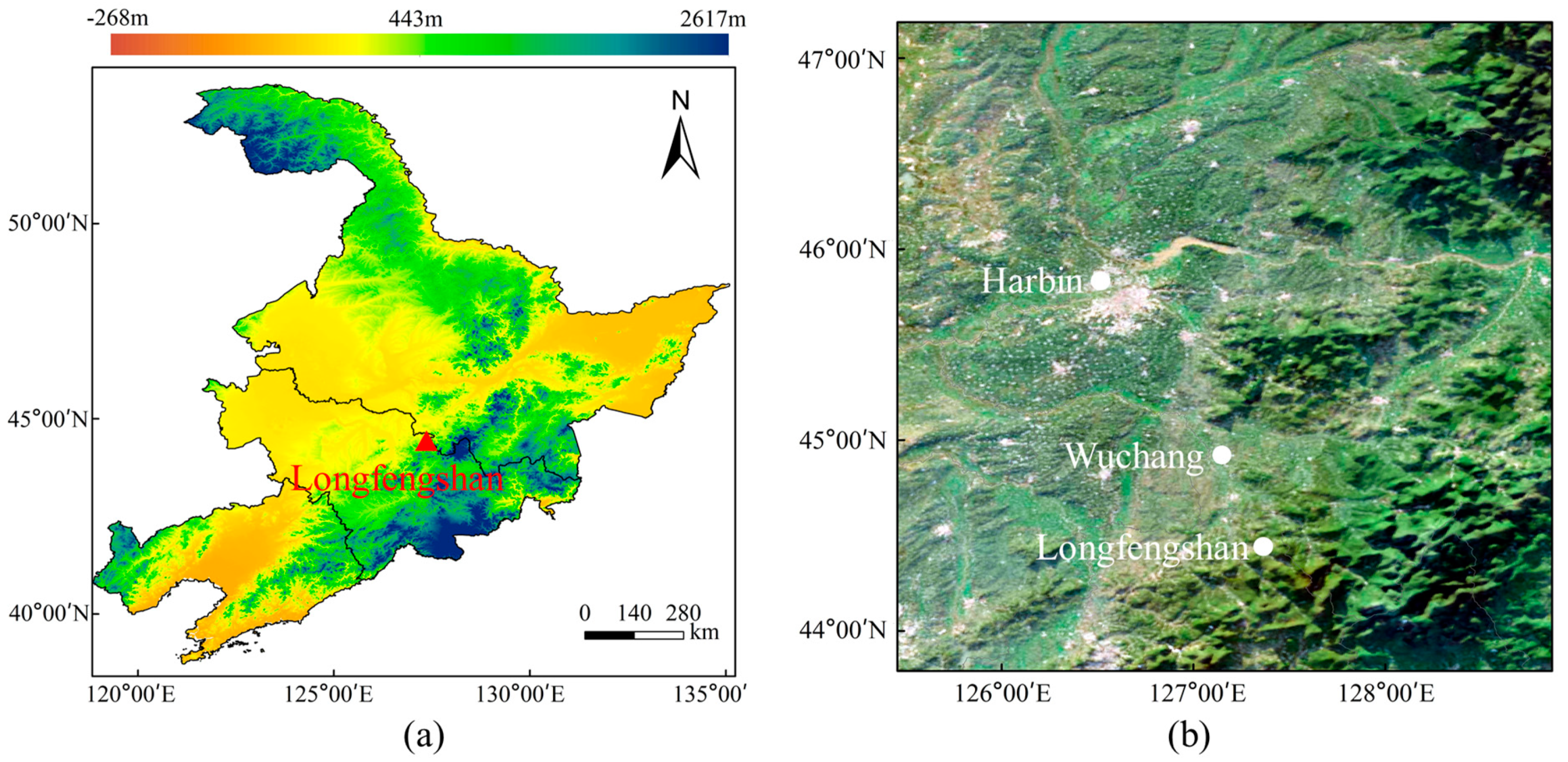
2.1. Site and Instrument

Ground-based MAX-DOAS measurements were performed at the Longfengshan (LFS) regional atmospheric background station (127°36′ E, 44°44′ N, 330.5 m a.s.l.) from 24 October 2020 to 13 October 2021 (with a break from 10 December 2020 to 3 March 2021 due to instrument malfunction). At present, the LFS station is the only background station under the framework of the WMO/GAW in the Northeast China [37]. The atmospheric observations started in 1991 at LFS [38], which represents the background atmospheric condition in the Northeast Plain region. The LFS station is located on the west side of Longfengshan reservoir, 60 km to the southeast of Wuchang City and 185 km to the southeast of Harbin City (Figure 1). It is located at the intersection of the Songnen plain and the Zhangguangcai ridge of the Changbai mountains. On the western side of the LFS station is the plain area, and on the eastern side is the mountainous forest area [39,40]. There are no villages in the range of 2 km away from the site, no high-density population, and no significant industrial emission sources in the range of 30 km away from the site [41].
We used a mini MAX-DOAS instrument from the Hoffmann Messtechnik GmbH, Germany, which was also used in our previous studies [24,36]. During the Second Cabauw Intercomparison Campaign for Nitrogen Dioxide Measuring Instruments (CINDI-2), the mean relative differences in the slant column from the reference value for the Mini MAX-DOAS were −2.10% for NO2 and −20.70% for HCHO [42]. The observation system consisted of an indoor section and an outdoor section. The outdoor section contains the entrance optics, fiber-coupled spectrograph, and controlling electronics inside a metal box. A stepper motor was installed outside the metal box to drive the instrument to rotate in the vertical direction for observation at different elevation angles [19]. In this study, each sequence contained 9 elevation angles (0°, 1°, 2°, 3°, 6°, 10°, 20°, 30°, and 90°), and it took about 4 min for a complete sequence. The spectrograph covered the wavelength range of 290–447 nm. A temperature control module was used to ensure that the spectrograph was operating at stable temperature lower than the ambient temperature. Solar scattering spectra were collected during the daytime period. The spectra of dark current and electron offset were also measured at specific operating temperatures, which were used to correct the measured spectra in the daytime and then reduce the influence of the spectrograph’s photoelectric noise [32]. More information about the instrumentation parameters can be found in the previous studies [31,43,44].

2.2. Spectral Analysis

According to the Beer–Lambert law, the differential slant column density (dSCD) can be retrieved from the measured scattering spectra by the DOAS method [19]. The dSCDs are the differences in slant column densities between the measured and reference spectra. The spectral analysis procedure was implemented by QDOAS software [45]. Before the spectral analysis, the spectra during the observation period were divided into 9 segments based on the operating temperature of the spectrograph. The observed spectra within each segment are corrected by using their corresponding spectra of dark current and electron offset. The high-resolution solar spectral were used for the wavelength calibration. NO2 and HCHO dSCDs were retrieved in wavelength ranges of 351~390 nm and 324~359 nm, respectively. The fitting parameters for NO2 and HCHO spectral analyses were similar as in previous studies [36,45,46], see Table 1. In this study, in order to improve the credibility of the data, only the spectra with root mean square (RMS) of the spectral fitting residuals < 0.003 and solar zenith angle (SZA) < 75° were retained [46,47]. Under the control of these two thresholds, we retained 70.67% of the NO2 profiles and 68.77% of the HCHO profiles. Figure 2 shows an example of spectral fitting for NO2 and HCHO dSCDs from the spectrum measured at 10:00 Beijing time (BJ, UTC + 8 h) on 5 July 2021 at an elevation angle of 10°.

2.3. Retrieval of NO2 and HCHO Vertical Profiles

The vertical profiles of NO2 and HCHO VMRs in the lower troposphere (0~4 km) were retrieved from the dSCDs by using the Profile inversion algorithm of aerosol extinction and the trace gas concentration algorithm (PriAM) [47]. The inversion consists of two procedures. In the first step, the vertical profiles of aerosol extinction (AE) were retrieved from the measured O4 dSCDs. Then the retrieved AE profiles were used for the inversion of the trace gas profiles [45,47]. For HCHO, the AE profiles at 360 nm were transformed into profiles at 343 nm by using the Ångström exponent. In this study, we set the Ångström exponent as 0.7, which was estimated based on the ERA5 reanalysis data. The entire observation period was divided into six segments according to the working temperature of the spectrograph. The inversion parameters of surface albedo, single scattering albedo, and asymmetry factor were listed in Table 2.
The PriAM algorithm was based on the optimal estimation method to obtain the vertical profiles via loop iteration, which minimized the parameter of cost function [47,52]. The smaller values of the cost function correspond to the more reliable retrieval results. The relative deviations of dSCDs reflect the differences between the PriAM and MAX-DOAS measurements. In order to balance the data quality and quantity, we retained the profiles with cost function < 30 and dSCDs relative deviations < 45% during the post-processing. With respect to the selected thresholds, 61.72% of NO2 profiles and 51.71% of HCHO profiles were left.

2.4. Ancillary Datasets

The in situ NO2 concentration and meteorological data such as surface temperature, relative humidity, and wind speed used in this study were derived from synchronous operational observations at the LFS station. Surface temperature, relative humidity, and wind speed were measured using an automatic meteorological station (DZZ5, Huayun Sonding, China), with precisions of ± 0.1 °C, ± 1%, and ± 0.1 m/s, respectively. The meteorological measurements follow the standard (QX/T 61−2007). The Ångström exponent, surface albedo, planetary boundary layer height (PBLH), and temperature–pressure a priori profiles were obtained from ERA5 reanalysis data (https://www.ecmwf.int/en/forecasts/dataset/ecmwf-reanalysis-v5, accessed on 25 May 2021). The asymmetry factor, single scattering albedo, and Ångström exponent were also referred to the data from the Aerosol Robotic Network (AERONET, https://aeronet.gsfc.nasa.gov/, accessed on 26 May 2021). The instrument used in the AERONET network was the CE318 multi−wavelength solar photometer (CIMEL, Paris, France).

3. Results

3.1. Overview

The averaged NO2 and HCHO vertical profiles below 4 km for the whole observation period are shown by the lines with dots in Figure 3. The NO2 VMR has the largest value at the surface and decreases with increasing altitude. There is an elevated HCHO pollution layer with VMRs larger than 2 ppb around the altitudes of 1.4 km. The means ± standard deviations of NO2 and HCHO VCDs are 4.69 ± 3.72 × 10¹⁵ and 1.19 ± 0.84 × 10¹⁶ molecule·cm−2, respectively. Correspondingly, the near-surface VMRs are 1.22 ± 1.09 ppb for NO2 and 2.41 ± 3.26 ppb for HCHO. The near-surface VMRs of NO2 and HCHO in this study are higher than those of NO2 (7~100 ppt) and HCHO (0.9 ppb) at the Waliguan regional atmospheric background station from 2012 to 2015 [36].

3.2. Temporal Variations

3.2.1. Monthly Variations

The monthly variations of the vertical profiles were different between NO2 and HCHO (Figure 4). The larger NO2 VMRs occur at the near-surface and decrease with increasing altitudes each month. The NO2 VMRs were lower in the lower troposphere in summer than in other seasons. For HCHO, larger VMRs appear not only near the surface but also at upper levels (~1.4 km altitude) in most observational months.
The maxima (minimum) of monthly averaged NO2 near-surface VMRs (Figure 4a) and VCDs (Figure 5a) were 2.51 ppb (0.47 ppb) and 8.6 × 10¹⁵ molecule·cm−2 (2.00 × 10¹⁵ molecule·cm−2) in November 2020 (August 2021). Tropospheric NO2 VCD shows a monthly variation trend of being higher in colder months and lower in warmer months (Figure 5a). The open burning of straw in autumn and the burning of fuel for heating in winter probably lead to an increase in NO2 emissions compared to summer. The cold and dry atmospheric conditions in autumn and winter are not conducive to gas spreading, resulting in the highest NO2 concentrations in autumn and winter [53].
The monthly HCHO VCDs maintained a high level from March to July 2021, with a maximum of 1.45 × 10¹⁶ molecule·cm−2 in June (Figure 5b). The HCHO minimum for both near-surface VMRs (1.12 ppb, Figure 4b) and VCDs (6.83 × 10¹⁵ molecule·cm−2, Figure 5b) appeared in October 2021. The near-surface HCHO VMRs were enhanced from late October to early December 2020, probably due to increased primary HCHO emissions from fossil fuel combustion in North China during the heating period [54]. The HCHO vertical distribution and column were influenced by complex factors, such as primary source from fossil fuel combustion [8] and secondary sources from chemical oxidation reactions [9]. The causes of HCHO temporal variation should be further investigated by comprehensive observation in future.

3.2.2. Diurnal Variations

In this study, we use April, July, and October 2021 as representatives of spring, summer, and autumn, respectively. The sample number in winter was too small to be discussed here. Figure 6 shows the diurnal variations of the vertical profile of NO2 and HCHO VMRs in April, July, and October 2021. High near-surface NO2 VMRs occurred in the early morning (5:00–9:00 BJ) and late evening (15:00–17:00 BJ) during April and July, but were stable throughout the daytime in October. In all three months, a polluted layer of NO2 was present in the residual layer. The planetary boundary layer developed to a maximum at 13:00 BJ. The elevated layer of NO2 disappeared gradually as the planetary boundary layer developed. The elevated layer existed throughout the day. Active photochemical reactions in the upper planetary boundary layer can contribute to the persistence of the HCHO elevation layer in the afternoon [55]. This characteristic is consistent with our observations at Raoyang meteorological station [46].
The daily variations of NO2 and HCHO VCDs are shown in Figure 7. NO2 VCDs remained at almost the same level throughout the day in April, with a slight increase after 14:00 BJ. In July, NO2 VCDs slightly decreased from 5:00 to 9:00 BJ, stayed almost the same from 10:00 to 15:00 BJ, and then increased slightly after 16:00 BJ. In October, NO2 VCDs were nearly constant throughout the day. The NO2 diurnal patterns were different from those in urban areas, where there are two peaks in the morning and evening due to traffic emissions [56]. For all three months, the NO2 diurnal variations ranges were small, implying that the local anthropogenic emission and photochemical reactions were weak at the LFS background station.
In April, HCHO VCDs varied gently during the period from 06:00 to 12:00 BJ and started to increase at 12:00 BJ until they reached the highest value at 16:00 BJ. In July, HCHO concentrations were high in the morning and evening but low at noon, with the maximum value appearing at 05:00 BJ. HCHO VCDs decreased to a minimum at 12:00 BJ and remained stable until 15:00 BJ. By comparing with the corresponding temperature and relative humidity qualitatively (Figure 8), we found that high NO2 VCDs tended to occur at low temperatures and high humidity, but this relationship was not found between HCHO and temperature. Because of the low wind speeds, the LFS station was mainly influenced by emissions from local sources.

3.3. HCHO/NO2 Ratio

3.3.1. Temporal Variation

The production of tropospheric ozone (O3) in most regions is associated with VOCs and NOx [57]. The ratio of HCHO to NO2 is an effective indicator for investigating the sensitivity of chemical ozone production to nitrogen oxides (NOx) and VOCs [46,58,59]. “RA” is used to refer to the ratio of HCHO to NO2, either in VMRs (RAVMR) or tropospheric VCD (RAVCD). According to previous studies, O3 production can be divided into VOCs-limited (RA < 1), transition zone (1 < RA < 2) and NOx-limited (RA > 2) [60,61]. In this study, in order to balance the quality and quantity of the data, only HCHO VMRs between 1 and 10 ppb and NO2 larger than 0.1 ppb were considered for the calculation of RA [46].
RA with respect to VMR has an elevated layer at the altitude of around 1.5 km (Figure 9a). The vertical distribution of the monthly means of RA (Figure 9b) shows that the height of the lower boundary of the elevated RA fell from October 2020 (1.2 km) to May 2021 (0.8 km). The larger RA filled the entire lower troposphere (below 2 km) from June until September 2021. In October 2021, RA in the lower troposphere decreased, and the lower boundary of the elevated layer rose again to 1.2 km. The majority of RA were less than 2 above the altitude of 2 km and less than 1 above the altitude of 2.5 km. The RAs of near-surface VMR and tropospheric VCD had the same seasonal variation patterns, with annual averages of 2.97 ± 3.04 for near-surface VMR and 4.03 ± 3.63 for tropospheric VCD (Figure 9c). The largest values of both RAVMR and RAVCD appeared in July, being 6.25 ± 4.00 and 8.22 ± 3.62, respectively. Correspondingly, the lowest RA appeared in December with the values of 0.96 ± 0.36 for RAVMR and 1.53 ± 0.67 for RAVCD.
The diurnal variation patterns of RA vertical distribution varied with seasons (Figure 10). In each month, the elevated layer of RA appeared around the altitudes of 1.5 km. In April, the RA was mainly between 1 and 2 in the lower boundary layer (0–0.4 km), with RA < 1 above 2.5 km. In July, RA > 2 filled the entire boundary layer (up to 2 km), with RA < 2 only appearing above 2 km. In October, RA was almost between one and two near the surface. The RAVCD was larger than two in all the three months. On average, the RA in July was ~3.2 and ~2.8 times higher than that in April and October, respectively.

3.3.2. Implication for O3 Production

To analyze the sensitivities of O3 production to the ratio of HCHO to NO2, we assume that daily O3 production at the LFS is approximately equal to the range of daytime O3 concentration variations at the surface, considering that the photochemical O3 production was a strong driver of the diurnal surface O3 variation [46,59]. Figure 11 shows the daily O3 production as a function of the daily average values of HCHO and NO2 for near-surface VMR (Figure 9a) and VCD (Figure 9b) during the daytime (05:00 to 17:00 BJ). The distribution patterns of O3 production, as classified by RAVMR and RAVCD, are similar. For most of the days, O3 production was concentrated in the NOx-limited regions or transition regions. On only a few days was the weaker O3 production (<20 ppb d−1) located in the VOCs-limited regions. Differently, the strongest near-surface O3 production occurred in the transition region for RAVMR, but in the NOx-limited region for RAVCD. From October 2020 to March 2021, the RAVMR varied between 1 and 2, implying that O3 production was in the transition regime. As a whole, O3 production was in the NOx-limited regime.

3.3.3. Relationship to Meteorological Conditions

The correlation coefficient between RAVMR and temperature (relative humidity) is 0.62 (0.53), implying that O3 production at LFS tended to be in the NOx−limited region when the temperature and relative humidity were higher (Figure 12a, b). In July, the temperature and relative humidity were high, and the RA was basically larger than two. There is no correlation relationship between RAVMR and wind speed (Figure 12c), with the correlation coefficient of 0.01 (not shown in figure). However, the RAVMR is dependent on the wind directions (Figure 12d–f). In April, maximum frequencies for RAVMR ≥ 2 and 1 < RAVMR < 2 were 14.81% in the SSW sector and 11.11% in the NNW sectors. Almost all the RAVMR values in July were larger than two and distributed in the SE–WSW sectors, with the largest frequency occurring in the S direction. In October, the largest frequency for RAVMR > 2 was 33.33% in the SSW direction and the frequencies for 1 < RAVMR < 2 were smaller and in the N and ESE directions. As a whole, the sensitivity of O3 production to NO2 and HCHO is closely related to temperature and relative humidity. Air masses from different directions can lead to different sensitivities of O3 production to NOx and VOCs at LFS Station.

4. Discussion

The averaged NO2 VCDs (4.69 × 10¹⁵ molecule·cm−2) during our observation period are larger than the mean level (1.16 × 10¹⁵ molecule·cm−2) in Heilongjiang province from 2005 to 2015 [60]. However, the mean HCHO VCDs in this study (1.19 × 10¹⁶ molecule·cm−2) are lower than those (1.39 × 10¹⁶ molecule·cm−2) in Heilongjiang province from 2005 to 2018 [61]. The background levels of NO2 and HCHO at LFS are useful to investigate as long-term trends in future studies.
The ranges of diurnal variation of NO2 VCDs are smaller at the LFS station than at another WMO/GAW background region in the North China Plain [35]. The vertical profile structures of both NO2 and HCHO at LFS in summer are similar to those observed at Raoyang, a rural site in the North China Plain [46]. The MAX−DOAS measurements at Raoyang were performed only for a summer period, and the elevated HCHO layer can be attributed to the air pollution and oxidization process in the lower atmosphere in the North China Plain [55]. The causes of larger VMRs at upper levels (~1.4 km altitude) at the LFS background station need to be fully understood in future studies.
Meteorological conditions affected the concentration levels, vertical distribution, and temporal variations of NO2 and HCHO, as well as the sensitivity of O3 production at the LFS station. There are at least three reasons: (1) The boundary layer evolution led to the vertical mixing of air masses; (2) The temperature and relative humidity affected the efficiency of O3 photochemical processes and the natural source emission; (3) Different wind speeds and directions were accompanied by air masses with different pollution levels.

5. Conclusions

We carried out MAX−DOAS observations at the Longfengshan regional atmospheric background station in Heilongjiang Province of China from October 2020 to October 2021, performed the spectral analysis with QDOAS software, and retrieved vertical profiles of NO2 and HCHO by using the PriAM algorithm. We explored the concentration, temporal, and spatial variation of NO2 and HCHO, and the sensitivity of O3 production to the ratio of HCHO to NO2. The conclusions are as follows:
The average levels of near-surface VMRs for NO2 and HCHO were 1.22 ± 1.09 ppb and 2.41 ± 3.26 ppb throughout the observation period, respectively. The NO2 vertical structure shows a declining pattern with increasing altitude, while HCHO has an elevated layer around the altitude of 1.4 km.
The NO2 VMRs in the lower troposphere tend to be higher in colder months and lower in warmer months at the LFS station. HCHO has an opposite monthly trend, especially at upper levels (~1.4 km altitude). There was a polluted layer of NO2 in the residual layer, which disappeared gradually with the development of planetary boundary layer. However, the HCHO elevated layer maintained throughout the daytime. Different from the gentle diurnal variations of NO2 VCDs, the HCHO VCDs are high in the morning and evening but low at noon in July. The qualitative comparisons show that high NO2 VCDs tended to occur at low temperatures and high humidity, but this relationship is not found for HCHO.
Although there were monthly and diurnal variations in the vertical profiles of the VMR ratio of HCHO to NO2, on most of the days, O3 production was in the NOx-limited regions or transition regions at the LFS station. There were only a few days of the experiment time when the weaker O3 production (<20 ppb) was located in the VOCs-limited regions. Besides the dependencies of wind direction, the O3 production at the LFS tended to be in the NOx-limited region when the temperature and relative humidity were higher.
The results of this study will be helpful for better understanding the spatiotemporal distribution characteristics of NO2 and HCHO in the background region, in addition, more comprehensive observations, such as concurrent measurements of O3 and VOCs together with MAX-DOAS, are recommended, which are significant for evaluating and designing the strategies for controlling O3 pollution.

Supplementary Materials

The following supporting information can be downloaded at: https://www.mdpi.com/article/10.3390/s23063269/s1.

Author Contributions

Conceptualization, S.L., S.C., J.M., and X.X.; methodology, S.L., S.C., and J.M.; validation, X.X., X.D., and D.Y.; formal analysis, S.L., S.C., and J.M.; investigation, S.L., J.G., J.L., and J.J.; resources, X.X. and J.M.; data curation, S.L., S.C., and J.M.; writing—original draft preparation, S.L.; writing—review and editing, S.L., S.C., J.M., and X.X.; visualization, S.L.; supervision, J.M.; project administration, X.X.; funding acquisition, J.M., X.X., and S.C. All authors have read and agreed to the published version of the manuscript.

Funding

This research was funded by the State Key Laboratory of Applied Optics (No. SKLAO2021001A02) and S&T Development Fund of CAMS (2020KJ003).

Institutional Review Board Statement

Not applicable.

Informed Consent Statement

Not applicable.

Data Availability Statement

Data sharing not applicable.

Acknowledgments

We thank the staff at the Longfengshan regional atmospheric background station for supporting the measurements. We thank BIRA-IASB for QDOAS spectral analysis software. We thank MPIC and AIOFM for PriAM algorithm. We thank ECMWF for providing reanalysis meteorological products.

Conflicts of Interest

The authors declare no conflict of interest. The funders had no role in the design of the study; in the collection, analyses, or interpretation of data; in the writing of the manuscript; or in the decision to publish the results.

References

  1. Seinfeld, J.H.; Pandis, S.N. Atmospheric Chemistry and Physics: From Air Pollution to Climate Change, 2nd ed.; John Wiley & Sons, Inc.: Hoboken, NJ, USA, 2006. [Google Scholar]
  2. Logan, J.A. Nitrogen oxides in the troposphere: Global and regional budgets. J. Geophys. Res. 1983, 88, 10785–10807. [Google Scholar] [CrossRef]
  3. Luo, C.; Zhou, X. The Study of The Cycle of Nitrogen Oxides in The Troposphere. Q. J. Appl. Meteorol. 1993, 4, 92–99. [Google Scholar]
  4. Brimblecombe, P.; Chu, M.; Liu, C.-H.; Fu, Y.; Wei, P.; Ning, Z. Roadside NO2/NOx and primary NO2 from individual vehicles. Atmos. Environ. 2023, 295, 119562. [Google Scholar] [CrossRef]
  5. Bauwens, M.; Compernolle, S.; Stavrakou, T.; Müller, J.F.; Gent, J.; Eskes, H.; Levelt, P.F.; Van Der A, R.; Veefkind, J.P.; Vlietinck, J.; et al. Impact of Coronavirus Outbreak on NO2 Pollution Assessed Using TROPOMI and OMI Observation. Geophys. Res. Lett. 2020, 47, e2020GL087978. [Google Scholar] [CrossRef] [PubMed]
  6. Labzovskii, L.D.; Belikov, D.A.; Damiani, A. Spaceborne NO2 observations are sensitive to coal mining and processing in the largest coal basin of Russia. Sci. Rep. 2022, 12, 12597. [Google Scholar] [CrossRef] [PubMed]
  7. Agency, E. Nitrogen Oxides (NOx), Why and How They Are Controlled; DIANE Publishing: Collingdale, PA, USA, 1999. [Google Scholar]
  8. Peng, W.; Wang, Y.; Gao, X.; Jia, S.; Xu, X.; Cheng, H.; Meng, Z. Characteristics of Ambient Formaldehyde at Two Rural Sites in the North China Plain in Summer. Res. Environ. Sci. 2016, 29, 1119–1127. [Google Scholar] [CrossRef]
  9. Wang, S.; Wang, H.; Liu, B. Determination of Atmospheric Formaldehyde in Beijing by High-Performance Liquid Chromatography. Res. Environ. Sci. 2008, 21, 27–30. [Google Scholar] [CrossRef]
  10. Parrish, D.D.; Ryerson, T.B.; Mellqvist, J.; Johansson, J.; Herndon, S.C. Primary and secondary sources of formaldehyde in urban atmospheres: Houston Texas region. Atmos. Chem. Phys. 2012, 12, 3273–3288. [Google Scholar] [CrossRef]
  11. Kaiser, J.; Jacob, D.J.; Lei, Z.; Travis, K.R.; Fisher, J.A.; Abad, G.G.; Lin, Z.; Zhang, X.; Fried, A.; Crounse, J.D. High-resolution inversion of OMI formaldehyde columns to quantify isoprene emission on ecosystem-relevant scales: Application to the southeast US. Atmos. Chem. Phys. 2018, 18, 5483–5497. [Google Scholar] [CrossRef]
  12. Jin, X.; Fiore, A.; Boersma, K.F.; Smedt, I.D.; Valin, L. Inferring Changes in Summertime Surface Ozone-NOx-VOC Chemistry over U.S. Urban Areas from Two Decades of Satellite and Ground-Based Observations. Environ. Sci. Technol. 2020, 54, 6518–6529. [Google Scholar] [CrossRef]
  13. Tan, Z.; Lu, K.; Jiang, M.; Su, R.; Dong, H.; Zeng, L.; Xie, S.; Tan, Q.; Zhang, Y. Exploring ozone pollution in Chengdu, southwestern China: A case study from radical chemistry to O3-VOC-NOx sensitivity. Sci. Total Environ. 2018, 636, 775–786. [Google Scholar] [CrossRef]
  14. Zhang, Y.; Li, Z.; Zhao, S.; Zhang, X.; Lin, J.; Qin, K.; Liu, C.; Zhang, Y. A review of collaborative remote sensing observation of atmospheric gaseous and particulate pollution with atmospheric environment satellites. Natl. Remote Sens. Bull. 2022, 5, 873–896. [Google Scholar]
  15. Cheng, S.; Cheng, X.; Ma, J.; Xu, X.; Zhang, W.; Lv, J.; Bai, G.; Chen, B.; Ma, S.; Dörner, S.; et al. Mobile MAX-DOAS observations of tropospheric NO2 and HCHO during summer over the Three Rivers’ Source region in China. Atmos. Chem. Phys. Discuss. 2022, 1–36. [Google Scholar] [CrossRef]
  16. Zhang, X.; Song, Q.; Gao, Y.; Wang, P.; Yu, D.; Wang, M.; Wen, M. Domestic in-situ Analyzer of Greenhouse Gases with Fourier Transform Infrared Spectroscopy and its Primary Application in Atmospheric Background Observation. J. Atmos. Environ. Opt. 2019, 14, 279–288. [Google Scholar] [CrossRef]
  17. Xu, J.; Xie, P.; Si, F.; Dou, K.; Li, A.; Liu, Y.; Liu, W. Retrieval of Tropospheric NO2 by Multi Axis Differential Optical Absorption Spectroscopy. Spectrosc. Spectr. Anal. 2010, 30, 2464–2469. [Google Scholar] [CrossRef]
  18. Wagner, T.; Dix, B.; Friedeburg, C.v.; Frieß, U.; Sanghavi, S.; Sinreich, R.; Platt, U. MAX-DOAS O4 measurements: A new technique to derive information on atmospheric aerosols—Principles and information content. J. Geophys. Res. 2004, 109, D22205. [Google Scholar] [CrossRef]
  19. Hönninger, G.; von Friedeburg, C.; Platt, U. Multi axis differential optical absorption spectroscopy (MAX-DOAS). Atmos. Chem. Phys. 2004, 4, 231–254. [Google Scholar] [CrossRef]
  20. Wittrock, F.; Oetjen, H.; Richter, A.; Fietkau, S.; Burrows, J.P. MAX-DOAS measurements of atmospheric trace gases in Ny-Ålesund- Radiative transfer studies and their application. Atmos. Chem. Phys. 2004, 4, 955–966. [Google Scholar] [CrossRef]
  21. Friedeburg, C.; Pundt, I.; Mettendorf, K.; Wagner, T.; Platt, U. Multi-axis-DOAS measurements of NO2 during the BAB II motorway emission campaign. Atmos. Environ. 2005, 39, 977–985. [Google Scholar] [CrossRef]
  22. Ang, L.; PinHua, X.; Cheng, L.; JianGuo, L.; WenQing, L. A Scanning Multi-Axis Differential Optical Absorption Spectroscopy System for Measurement of Tropospheric NO2 in Beijing. Chin. Phys. Lett. 2007, 24, 2859–2862. [Google Scholar] [CrossRef]
  23. Wang, Y.; Li, A.; Xie, P.-H.; Chen, H.; Mou, F.-S.; Xu, J.; Wu, F.-C.; Zeng, Y.; Liu, J.-G.; Liu, W.-Q. Measuring tropospheric vertical distribution and vertical column density of NO2 by multi-axis differential optical absorption spectroscopy. Acta Phys. Sin. 2013, 62, 200705. [Google Scholar] [CrossRef]
  24. Jin, J.; Ma, J.; Lin, W.; Zhao, H.; Shaiganfar, R.; Beirle, S.; Wagner, T. MAX-DOAS measurements and satellite validation of tropospheric NO2 and SO2 vertical column densities at a rural site of North China. Atmos. Environ. 2016, 133, 12–25. [Google Scholar] [CrossRef]
  25. Hendrick, F.; Müller, J.-F.; Clémer, K.; Wang, P.; Mazière, M.D.; Fayt, C.; Gielen, C.; Hermans, C.; Ma, J.Z.; Pinardi, G.; et al. Four years of ground-based MAX-DOAS observations of HONO and NO2 in the Beijing area. Atmos. Chem. Phys. 2014, 14, 765–781. [Google Scholar] [CrossRef]
  26. Tanvir, A.; Javed, Z.; Jian, Z.; Zhang, S.; Bilal, M.; Xue, R.; Wang, S.; Bin, Z. Ground-Based MAX-DOAS Observations of Tropospheric NO2 and HCHO During COVID-19 Lockdown and Spring Festival Over Shanghai, China. Remote Sens. 2021, 13, 488. [Google Scholar] [CrossRef]
  27. Xue, J.; Zhao, T.; Luo, Y.; Miao, C.; Su, P.; Liu, F.; Zhang, G.; Qin, S.; Song, Y.; Bu, N.; et al. Identification of ozone sensitivity for NO2 and secondary HCHO based on MAX-DOAS measurements in northeast China. Environ. Int. 2022, 160, 107048. [Google Scholar] [CrossRef]
  28. Ren, B.; Xie, P.; Xu, J.; Li, A.; Qin, M.; Hu, R.; Zhang, T.; Fan, G.; Tian, X.; Zhu, W.; et al. Vertical characteristics of NO2 and HCHO, and the ozone formation regimes in Hefei, China. Sci. Total Environ. 2022, 823, 153425. [Google Scholar] [CrossRef] [PubMed]
  29. Luo, Y.; Dou, K.; Fan, G.; Huang, S.; Si, F.; Zhou, H.; Wang, Y.; Pei, C.; Tang, F.; Yang, D. Vertical distributions of tropospheric formaldehyde, nitrogen dioxide, ozone and aerosol in southern China by ground-based MAX-DOAS and LIDAR measurements during PRIDE-GBA 2018 campaign. Atmos. Environ. 2020, 226, 117384. [Google Scholar] [CrossRef]
  30. Huang, X.; Shao, T.; Zhao, J.; Cao, J.; Song, Y. Spatio-temporal Differentiation of Ozone Concentration and Its DrivingFactors in Yangtze River Delta Urban Agglomeration. Resour. Environ. Yangtze Basin 2019, 28, 1434–1445. [Google Scholar] [CrossRef]
  31. Ma, J.; Beirle, S.; Jin, J.; Shaiganfar, R.; Yan, P.; Wagner, T. Tropospheric NO2 vertical column densities over Beijing: Results of the first three years of ground-based MAX-DOAS measurements (2008–2011) and satellite validation. Atmos. Chem. Phys. 2013, 13, 1547–1567. [Google Scholar] [CrossRef]
  32. Jin, J.; Ma, J.; Lin, W.; Zhao, H. Characteristics of NO2 Tropospheric Column Density over a Rural Area in the North China Plain. J. Appl. Meteorol. Sci. 2016, 27, 303–311. [Google Scholar] [CrossRef]
  33. Li, W.; Ma, J.; Guo, J. Measuring Atmospheric NO2 Column Densities by MAX-DOAS:Method and Application. Meteorol. Sci. Technol. 2013, 41, 796–802. [Google Scholar] [CrossRef]
  34. Chan, K.; Hartl, A.; Lam, Y.; Xie, P.; Liu, W.; Cheung, H.; Lampel, J.; Poehler, D.; Li, A.; Xu, J. Observations of tropospheric NO2 using ground based MAX-DOAS and OMI measurements during the Shanghai World Expo 2010. Atmos. Environ. 2015, 119, 45–58. [Google Scholar] [CrossRef]
  35. Cheng, S.; Ma, J.; Zhou, H.; Jin, J.; Liu, Y.; Dong, F.; Zhou, L.; Yan, P. Spectral Inversion and Characteristics of NO_2 Column Density at Shangdianzi Regional Atmospheric Background Station. Spectrosc. Spectr. Anal. 2018, 38, 3470–3475. [Google Scholar] [CrossRef]
  36. Ma, J.; Steffen, D.; Sebastian, D.; Jin, J.; Cheng, S.; Guo, J.; Zhang, Z.; Wang, J.; Liu, P.; Zhang, G.; et al. MAX-DOAS measurements of NO2, SO2, HCHO, and BrO at the Mt. Waliguan WMO/GAW global baseline station in the Tibetan Plateau. Atmos. Chem. Phys. 2020, 20, 6973–6990. [Google Scholar] [CrossRef]
  37. Wu, Y.; Ning, S.; Yu, D.; Song, Q.; Dai, X.; Zhao, J. Characteristics of CO2 concentrations and its variations at Longfengshan regional atmospheric background station in Northeast China. Environ. Chem. 2015, 34, 1627–1632. [Google Scholar] [CrossRef]
  38. Dai, X. Patterns of changes in background values of total ozone at Longfengshan regional background station. Sci. Technol. Innov. Her. 2008, 30, 177. [Google Scholar] [CrossRef]
  39. Yu, D.; Wu, Y.; Song, Q.; Dai, X.; Lin, W. Environmental Characteristics and Its Observations at Longfengshan WMO Regional Atmospheric Background Station. Clim. Change Res. Lett. 2012, 1, 65–73. [Google Scholar] [CrossRef]
  40. Xu, X.; Ding, G. Study on acidic gases in the regional background air in northeastern China. China Env. Ental Sci. 1997, 17, 345–348. [Google Scholar] [CrossRef]
  41. Yu, D.; Song, Q.; Sun, J.; Liu, J.; Wu, Y.; Xia, C. Characteristics of aerosol scattering coefficient at Longfengshan regional background station. Environ. Chem. 2019, 40, 765–771. [Google Scholar] [CrossRef]
  42. Kreher, K.; Roozendael, M.V.; Hendrick, F.; Apituley, A.; Zhao, X. Intercomparison of NO2, O4, O3 and HCHO slant column measurements by MAX-DOAS and zenith-sky UV-Visible spectrometers during the CINDI-2 campaign. Atmos. Meas. Tech. 2020, 13, 2169–2208. [Google Scholar] [CrossRef]
  43. Cheng, S.; Jin, J.; Ma, J.; Xu, X.; Ran, L.; Ma, Z.; Chen, J.; Guo, J.; Yang, P.; Wang, Y.; et al. Measuring the Vertical Profiles of Aerosol Extinction in the Lower Troposphere by MAX-DOAS at a Rural Site in the North China Plain. Atmosphere 2020, 11, 1037–1053. [Google Scholar] [CrossRef]
  44. Cheng, S.; Ma, J.; Cheng, W.; Yan, P.; Zhou, H.; Zhou, L.; Yang, P. Tropospheric NO2 vertical column densities retrieved from ground-based MAX-DOAS measurements at Shangdianzi regional atmospheric background station in China. J. Environ. Sci. 2019, 80, 186–196. [Google Scholar] [CrossRef] [PubMed]
  45. Platt, U. Differential Optical Absorption Spectroscopy (DOAS). Air Monit. By Spectrosc. Tech. 1994. [Google Scholar] [CrossRef]
  46. Wang, Y.; Dörner, S.; Donner, S.; Böhnke, S.; De Smedt, I.; Dickerson, R.R.; Dong, Z.; He, H.; Li, Z.; Li, Z.; et al. Vertical profiles of NO2, SO2, HONO, HCHO, CHOCHO and aerosols derived from MAX-DOAS measurements at a rural site in the central western North China Plain and their relation to emission sources and effects of regional transport. Atmos. Chem. Phys. 2019, 19, 5417–5449. [Google Scholar] [CrossRef]
  47. Cheng, S.; Jin, J.; Ma, J.; Lv, J.; Liu, S.; Xu, X. Temporal Variation of NO2 and HCHO Vertical Profiles Derived from MAX-DOAS Observation in Summer at a Rural Site of the North China Plain and Ozone Production in Relation to HCHO/NO2 Ratio. Atmosphere 2022, 13, 860. [Google Scholar] [CrossRef]
  48. Wang, Y.; Lampel, J.; Xie, P.; Beirle, S.; Li, A.; Wu, D.; Wagner, T. Ground-based MAX-DOAS observations of tropospheric aerosols, NO2, SO2 and HCHO in Wuxi, China, from 2011 to 2014. Atmos. Chem. Phys. 2017, 17, 2189–2215. [Google Scholar] [CrossRef]
  49. Wang, Y.; Li, A.; Xie, P.H.; Chen, H.; Xu, J.; Wu, F.C.; Liu, J.G.; Liu, W.Q. Retrieving vertical profile of aerosol extinction by multi-axis differential optical absorption spectroscopy. Acta Phys. Sin. 2013, 62, 180705. [Google Scholar] [CrossRef]
  50. Xiang, X.; Cui, Z.; Zhang, H.; Pei, L.; Chao, M. Analysis of Laws of NO2 Emission and Driving Factors of China’s Key Cities. Environ. Sci. Technol. 2022, 045, 30–45. [Google Scholar] [CrossRef]
  51. Yan, M.; Yang, N.; Zhong, S.; Wang, L. Research on meteorological indicators for heating decisions in Heilongjiang Province. Heilongjiang Meteorol. 2021, 38, 32–33, 41. [Google Scholar] [CrossRef]
  52. Ma, J.; Wang, Y. The IPAC-NC field campaign: A pollution and oxidization pool in the lower atmosphere over Huabei, China. Atmos. Chem. Phys. 2012, 12, 3883–3908. [Google Scholar] [CrossRef]
  53. Xu, H.; Liu, H.; Ji, X.; Li, Q.; Liu, G.; Ou, J. Observation of tropospheric NO2 using ground-based MAX-DOAS and OMI measurements during the Shanghai. Spectrosc. Spectr. Anal. 2022, 42, 2720–2725. [Google Scholar] [CrossRef]
  54. Sillman, S. The relation between ozone, NOx and hydrocarbons in urban and polluted rural environments. Atmos. Environ. 1999, 33, 1821–1845. [Google Scholar] [CrossRef]
  55. Ryan, R.G.; Rhodes, S.; Tully, M.; Schofield, R. Surface ozone exceedances in Melbourne, Australia are shown to be under NOx control, as demonstrated using formaldehyde:NO2 and glyoxal: Formaldehyde ratios. Sci. Total. Environ. 2020, 749, 141460. [Google Scholar] [CrossRef] [PubMed]
  56. Hong, Q.; Liu, C.; Hu, Q.; Zhang, Y.; Xing, C.; Su, W.; Ji, X.; Xiao, S. Evaluating the feasibility of formaldehyde derived from hyperspectral remote sensing as a proxy for volatile organic compounds. Atmos. Res. 2021, 264, 105771. [Google Scholar] [CrossRef]
  57. Duncan, B.N.; Yoshida, Y.; Olson, J.R.; Sillman, S.; Martin, R.V.; Lamsal, L.; Hu, Y.; Pickering, K.E.; Retscher, C.; Allen, D.J.; et al. Application of OMI observations to a space-based indicator of NOx and voe controls on surface ozone formation. Atmos. Environ. 2010, 44, 2213–2223. [Google Scholar] [CrossRef]
  58. Souri, A.H.; Nowlan, C.R.; Wolfe, G.M.; Lamsal, L.N.; Miller, C.E.C.; Abad, G.G.; Janz, S.J.; Fried, A.; Blake, D.R.; Weinheimer, A.J.; et al. Revisiting the effectiveness of HCHO/NO2 ratios for inferring ozone sensitivity to its precursors using high resolution airborne remote sensing observations in a high ozone episode during the KORUS-AQ campaign- ScienceDirect. Atmos. Environ. 2020, 224, 117341. [Google Scholar] [CrossRef]
  59. Ma, J.; Liu, H. Summertime tropospheric ozone over China simulated with a regional chemical transport model 1. Model description and evaluation. J. Geophys. Res. Atmos. 2002, 107, ACH 27:21–ACH 27:13. [Google Scholar] [CrossRef]
  60. Zhou, C.; Li, Q.; Zhang, L.; Ma, P.; Chen, H.; Wang, Z. Spatio-tenporal Change and Influencing Factors of Tropospheric NO2 Column Density of China during 2005~2015. Remote Sens. Technol. Appl. 2016, 31, 1190–1200. [Google Scholar] [CrossRef]
  61. Huang, S.; Li, N.; He, S.; Dong, H. Spatial-temporal Variations and Influencing Factors of Formaldehyde in the Three Provinces of Northeast China during 2005–2018. Earth Environ. 2020, 48, 652–662. [Google Scholar] [CrossRef]
Figure 1. (a) The elevation map of Longfengshan regional atmospheric background station. (b) The major neighborhood cities around the LFS station (the background image is from the Sentinel−2 satellite).
Sensors 23 03269 g001
Figure 2. Examples of spectral fitting for (a) NO2 and (b) HCHO. Black and red curves are the measured and fitted differential optical depths, respectively. The NO2 and HCHO dSCDs are 1.10 × 10¹⁶ molecule·cm−2 and 2.30 × 10¹⁶ molecule·cm−2, respectively. The RMS between measured and fitted spectra are 7.63 × 10⁻⁴ for NO2 and 8.98 × 10⁻⁴ for HCHO, respectively.
Sensors 23 03269 g002
Figure 3. Vertical profiles of NO2 (black) and HCHO (red) VMRs. The lines with dots and the error bars indicate the means and standard deviations at different altitudes during the observation period. The averaged values ± standard deviations of tropospheric NO2 and HCHO VCDs (Unit: 1015 molecule·cm−2) during the observation period are also shown in the figure.
Sensors 23 03269 g003
Figure 4. Monthly vertical profiles of (a) NO2 and (b) HCHO VMRs.
Sensors 23 03269 g004
Figure 5. Monthly tropospheric VCDs (Unit: 1015 molecule·cm−2) for (a) NO2 and (b) HCHO. The upper (lower) error bars and upper (lower) boundaries of the boxes are the 95th (5th) and 75th (25th) percentiles of the data grouped per month, respectively. The lines inside the boxes and the red curves with dots indicate the medians and the averages, respectively. The number of sampling days per month is marked on the top axis.
Sensors 23 03269 g005
Figure 6. Diurnal variations of the vertical profile of NO2 in April (a), July (c) and October (e). (b,d,f) Same as (a,c,e) correspondingly, but for HCHO. The red line indicates the planetary boundary layer height (PBLH).
Sensors 23 03269 g006
Figure 7. Diurnal variations of tropospheric VCDs for (a) NO2 and (b) HCHO. The dots denote the averages, and the error bars represent the 25th and 75th percentiles of the data grouped for each hour. The blue, red, and black dotted lines denote April, July and October 2021, respectively.
Sensors 23 03269 g007
Figure 8. Diurnal variations of temperature (black), relative humidity (red), wind speed and direction (blue) in (a) April, (b) July and (c) October 2021.
Sensors 23 03269 g008
Figure 9. (a) Vertical profiles of the ratio of HCHO to NO2 during the observation period. The dots and whiskers indicate the average of all data at selected altitudes during the observation period and the standard deviation, respectively. (b) Monthly variation of vertical profiles of VMRs ratios of HCHO to NO2. (c) Monthly variation of the ratio of HCHO to NO2 for tropospheric VCDs and near-surface VMRs. The dots and the error bars denote the averages and the 25th and 75th percentiles of the data grouped for each month. HCHO/NO2 = 1 and 2 are also marked with dashed lines. The white grid cells in panel (b) indicate the missing data owing to lacking observation and data quality control.
Sensors 23 03269 g009
Figure 10. Diurnal variations in the vertical profile of the ratio of HCHO to NO2 VMRs in (a) April, (b) July, and (c) October 2021. (d) Diurnal variations of RAVCD in April, July, and October 2021. The dots and error bars represent the averages and the 25th (75th) percentiles of the data grouped for each hour in April (blue), July (red) and October (black).
Sensors 23 03269 g010
Figure 11. (a) Daily average of near-surface VMRs for HCHO and NO2. (b) same as (a) but for VCDs, colored by the range of daytime surface O3 variation. The dashed lines indicate HCHO/NO2 = 1 and 2.
Sensors 23 03269 g011
Figure 12. Relationship between the near-surface VMR ratios of HCHO to NO2 and meteorological factors, i.e., (a) air temperature, (b) relative humidity, (c) wind speed, and (df) wind direction. The dots, triangles, and pentagrams represent April, July, and October 2021, respectively. Rose plots denote RAVMR frequencies in 16 wind directions in (d) April, (e) July and (f) October 2021.
Sensors 23 03269 g012
Table 1. Setting for NO2 and HCHO spectral analyses.
ParametersO4 and NO2HCHO
Fraunhofer referencesequential spectra
Fitting interval351~390 nm324~359 nm
DOAS polynomialdegree: 5
Intensity offsetdegree: 2 (constant and order 1)
Shift and stretchspectral
Ring spectraOriginal and wavelength-dependent Ring spectra
NO2 cross sectionVandaele et al. (1998) [48], 294 K, 220 K,
I0 correction (1017 molecule·cm−2)
Vandaele et al. (1998) [48], 294 K,
I0 correction (1017 molecule·cm−2)
O3 cross sectionSerdyuchenko et al. (2014) [49], 223 K,
I0 correction (1020 molecule·cm−2)
Serdyuchenko et al. (2014) [49], 223 K, 243 K,
I0 correction (1020 molecule·cm−2)
O4 cross sectionThalman and Volkamer (2013) [50], 293 K
HCHO cross sectionMeller and moortgat (2000) [51], 298 K
Table 2. Surface albedo, single scattering albedo, and asymmetry factor for each segment of profile inversion.
NO.Start and End TimeSurface AlbedoSingle Scattering AlbedoAsymmetry Factor
12020/10/26—2020/11/180.110.940.7
22020/11/19—2020/12/080.220.940.7
32021/03/04—2021/04/070.130.930.7
42021/04/07—2021/06/120.150.920.7
52021/06/13—2021/07/270.170.940.7
62021/08/01—2021/10/120.150.960.7
Disclaimer/Publisher’s Note: The statements, opinions and data contained in all publications are solely those of the individual author(s) and contributor(s) and not of MDPI and/or the editor(s). MDPI and/or the editor(s) disclaim responsibility for any injury to people or property resulting from any ideas, methods, instructions or products referred to in the content.

