Abstract
Minimally invasive surgery has undergone significant advancements in recent years, transforming various surgical procedures by minimizing patient trauma, postoperative pain, and recovery time. However, the use of robotic systems in minimally invasive surgery introduces significant challenges related to the control of the robot’s motion and the accuracy of its movements. In particular, the inverse kinematics (IK) problem is critical for robot-assisted minimally invasive surgery (RMIS), where satisfying the remote center of motion (RCM) constraint is essential to prevent tissue damage at the incision point. Several IK strategies have been proposed for RMIS, including classical inverse Jacobian IK and optimization-based approaches. However, these methods have limitations and perform differently depending on the kinematic configuration. To address these challenges, we propose a novel concurrent IK framework that combines the strengths of both approaches and explicitly incorporates RCM constraints and joint limits into the optimization process. In this paper, we present the design and implementation of concurrent inverse kinematics solvers, as well as experimental validation in both simulation and real-world scenarios. Concurrent IK solvers outperform single-method solvers, achieving a 100% solve rate and reducing the IK solving time by up to 85% for an endoscope positioning task and 37% for a tool pose control task. In particular, the combination of an iterative inverse Jacobian method with a hierarchical quadratic programming method showed the highest average solve rate and lowest computation time in real-world experiments. Our results demonstrate that concurrent IK solving provides a novel and effective solution to the constrained IK problem in RMIS applications.
1. Introduction
Minimally invasive surgery (MIS) is a standard surgical procedure that reduces trauma and accelerates recovery by using long and thin surgical instruments through small incisions to access the anatomy of the patients. However, loss of direct access to the surgical workspace and the limited dexterity of conventional surgical tools impose several challenges on the surgeon, including a lack of depth perception and haptic feedback [1], which increases cognitive workload. To overcome these limitations, there has been increasing interest in the development of robotic systems for robot-assisted minimally invasive surgery (RMIS), as they enhance the surgeon’s capabilities with 3D vision, dexterous surgical tools, and intuitive human–robot interfaces. Numerous robotic systems have been developed and studied in the literature. The most prominent example is the da Vinci surgical system [2], which has been widely adopted in numerous surgical rooms around the world and has performed diverse surgical procedures in different anatomical regions, such as laparoscopic, gynecological and general surgery [3]. The da Vinci surgical system employs multiple robotic arms, each equipped with a surgical instrument that accesses internal organs through trocars placed over the patient’s body. However, the da Vinci surgical system has a bulky setup, entails a high cost, and the dimensions of the robotic surgical tool make it unsuitable for all types of surgery. To address these limitations, novel robotic surgical systems have been proposed for specific surgical scenarios, such as eye surgery [4], transnasal surgery [5], or pediatric laparoscopic surgery [6].
A key constraint in RMIS is the requirement for a remote center of motion (RCM), which is a constraint located at the insertion point, typically a trocar, that must always be respected. The surgical tool must pivot over the RCM, limiting its mobility to four degrees of freedom (DOFs): translational motion along the tool axis, pitch and yaw rotations, and rotational motion along the tool axis. Various strategies have been proposed to ensure the RCM constraint and can be coarsely classified as mechanical and programmable RCMs [7]. RCM mechanisms typically use structures based on parallelograms, which facilitate motion control and prevent potential hazards by ensuring the constraint of the RCM at the mechanical level [8,9]. However, mechanical RCMs have a significant limitation in their lack of adaptability, as the location of the RCM is fixed and must be aligned with the trocar placed on the patient. As a result, the placement of the robotic system, as well as the layout of the surgical room, must be adapted to accommodate the mechanical structure. Moreover, the RCM mechanism occupies a considerable amount of space above the insertion point, limiting robotic arms’ range of motion and obstructing the assistant staff’s access. The da Vinci surgical system [10] is an example of a passive RCM. On the contrary, programmable RCMs offer flexibility with a software-based RCM that can be dynamically adjusted without the need for additional mechanical structures, which also reduces costs. It utilizes the redundancy found in typical robotic manipulators to keep the constraint through synchronized control of the manipulator’s joints. The DLR MIRO [11] is an example of a surgical robotic system that follows a programmable RCM strategy. However, this approach transforms the RCM problem into a control problem that requires real-time motion planning to solve.
The emergence of various robot configurations designed for specific surgical applications, each with different kinematic chains and kinematic constraints, makes it even more challenging to solve the programmable RCM problem using a single general approach. Consequently, each robotic system has to develop its own case-specific motion control strategy. This study aims to introduce a general framework that addresses the constrained inverse kinematic problem for robot-assisted surgical applications. The main contributions of this work are threefold:
- A novel concurrent inverse kinematics framework that combines classical Inverse Jacobian IK and optimization-based IK approaches, which delivers high solving rates and improved time performance.
- A benchmark that allows the proposed method to be compared with conventional approaches.
- Experimental validation in typical applications of RMIS with multiple kinematic robot structures.
To facilitate reproducibility and further research, we made the code for the IK solvers implementation, benchmark, and simulation environments publicly available at https://github.com/jcolan/CoIKS (accessed on 19 March 2023).
2. Related Works
2.1. Constrained Inverse Kinematics
Inverse kinematics is a fundamental problem in robotics, which involves determining the joint angles necessary to achieve a desired position and orientation of the end effector. For non-redundant manipulators, analytical approaches provide explicit solutions for the unconstrained inverse kinematics problem. However, when the robot has redundant degrees of freedom, the inverse kinematics problem becomes more complex, as there can be multiple kinematic solutions. Additionally, the problem can become more challenging when there are additional tasks and kinematic constraints that must be satisfied, such as obstacle avoidance or joint limits. In such cases, iterative numerical methods or optimization techniques are often used to find a suitable solution.
Constrained inverse kinematics is a critical building block for developing control strategies for robotic systems that must accomplish multiple tasks simultaneously. It has been extensively studied for various types of constraints, such as joint limits avoidance [12], obstacle avoidance [13], robot posture [14], and maximization of manipulability [15]. Kinematic redundancy, which occurs when the manipulator’s degrees of freedom are greater than those required to execute a task, is often utilized to satisfy these additional constraints [16].
Analytical approaches are commonly used to solve the constrained inverse kinematics problem [17,18]. Although they can provide closed-form solutions suitable for real-time robot control, the set of constraints that analytical IK solvers can handle is limited. Additionally, analytical solvers must be designed in advance and can be susceptible to changes in robot configuration.
Numerical solvers, on the other hand, are more generic and use iterative methods based on the local Jacobian inverse until convergence to an optimal solution. Numerical IK solvers are known to be slower than analytical methods, and active research has been carried out to speed up the solving time by looking for alternatives to Jacobian inverse computation [19] or combining it with other optimization-based methods [20]. Generic constraints can be included in an optimization-based numerical approach, in which the IK problem is formulated as a general nonconvex nonlinear optimization problem and solved by iterative gradient-based nonlinear solvers [21]. This approach can handle a wide range of constraints, including nonlinear and nonconvex ones, and is suitable for a variety of robotic applications. However, it can be computationally expensive and may require careful tuning of the solver parameters to achieve the desired performance.
2.2. Task Prioritization
When a hierarchy exists between constraint tasks in inverse kinematics, a prioritization scheme must be followed. Each task is assigned a priority level, and high-priority tasks should not be affected by lower-priority tasks [22]. There are two main categories of hierarchical IK schemes: strict and non-strict control methods.
Strict methods assume that each task is assigned a different priority, enforcing the hierarchy by projecting consecutively joint velocities from lower-priority tasks to the null space of higher-priority tasks. Siciliano and Slotine [23] proposed a hierarchical framework to handle an arbitrary number of tasks by considering the null space projector of one task in the next task solution in priority order. Chiaverini [24] proposed a different approach for two tasks that guarantees robustness against algorithmic singularity, which is later extended to multiple tasks in [25]. Hierarchical quadratic programming (HQP) has also been explored for strict hierarchical IK, solving a quadratic programming problem hierarchically under equality and inequality constraints. HQP has been used in humanoid robots [26], robot teleoperation [27], and human–robot collaboration [28].
Non-strict methods offer a simplified approach to task prioritization by assigning weights to each task according to its relative importance. This simplification reduces computational time and allows for more flexible control over the optimization problem. However, in cases where multiple tasks have the same priority level, non-strict methods can result in ambiguity and compromise the desired priority scheme. Additionally, it is challenging to completely isolate one task from the influence of another, even when assigning vastly different weights. A critical drawback of non-strict methods is the need for fine-tuning the weight assignment for each task, which can be time consuming and require expert knowledge.
2.3. Constrained Inverse Kinematics in RMIS
In RMIS, the preservation of the remote center of motion (RCM) is an essential constraint that must be addressed. Typically, programmable RCM constraints are formulated as high-priority tasks within a strict hierarchical control scheme. For instance, Azimian et al. [29] proposed a method that utilizes a projection of a secondary tool pose control task in the null space of the RCM task. The RCM constraint task is described as a kinematic restriction based on the plane tangent to the patient’s skin. They experimentally validated their approach in an endoscope positioning task. However, one of the limitations of their method is the assumption of constant tool insertion depth, which may not hold throughout the surgical procedure. To overcome this limitation, Aghakhani et al. [30] proposed a variation of the previous method, which considers the tool insertion velocity as an additional control variable. They utilize an augmented Jacobian approach in which the tool pose control task and the RCM constraint task Jacobians are stacked. The pseudoinverse of the augmented Jacobian provides a solution that satisfies both tasks. However, their method does not ensure the orthogonality of both task Jacobians, which can lead to algorithmic singularities in the augmented task Jacobian [31]. Another strict hierarchical approach was proposed by Sandoval et al. [32] for a torque-controlled manipulator. In their approach, they prioritize the task of minimizing the distance between the trocar point and the surgical tool, while a secondary task is defined as the control of the tool pose. Following this approach, they were able to achieve an accurate position of the tool tip while ensuring the preservation of the RCM.
While some approaches for RCM implementations consider independent tasks in a hierarchical scheme, others aim to unify the task. For example, Osa et al. [33] introduced a zero-velocity constraint in the normal plane of the tool axis to avoid lateral movement around the RCM. Marinho et al. [34] proposed generating a trajectory by projecting the desired endoscope position from the perspective of the RCM, then computing the corresponding joint configurations for the external joints. However, these methods have limitations, including their dependence on the number of links within the patient. For example, refs. [33,34] only consider one link after the trocar point, and joint limits are not directly taken into account in the RCM formulation.
Optimization-based RCM formulations can explicitly incorporate equality and inequality constraints, making them suitable for including joint limits in the problem. In [35], Kapoor et al. proposed a weighted multi-objective constrained optimization framework that uses a sequential quadratic programming approach to solve the nonlinear constrained problem. Yang et al. [36] employed a differential evolution algorithm to solve an endoscope visual servoing optimization problem subject to an RCM constraint.
To address the constrained inverse kinematics problem for serial manipulators with general kinematic structures, including highly redundant manipulators with multiple links within the patient, which has yet to be extensively studied, this work presents a novel concurrent inverse kinematic framework.
3. Concurrent Inverse Kinematic Solvers
Concurrent inverse kinematic (IK) solving has been proposed as a technique to significantly improve the success rate and execution time for solving multiple kinematic chains, as demonstrated in TRAC-IK [20]. However, TRAC-IK is not designed for multiple tasks or to incorporate additional constraints, such as RCM for RMIS. To overcome this limitation, we propose an extension of concurrency solving that takes into account the unique constraints present in RMIS. Specifically, our approach combines the Inverse Jacobian method with hierarchical quadratic programming and nonlinear optimization for concurrent IK solving, which explicitly incorporates RCM constraints into the optimization process. While Inverse Jacobian-based IK solvers can suffer from instabilities and local minima, optimization-based IK solvers can be slower but can explicitly include constraints and are better at avoiding local minima. To improve the IK solving performance, we proposed a combination of both strategies with a concurrent multi-threaded deployment of IK solvers. This enables us to solve the constrained IK problem in RMIS with higher success rates and reduced computational time. We evaluated three single-method IK-solving strategies and four concurrent IK solvers implemented based on the previous single IK solvers listed as follows:
- INVJ: Inverse Jacobian IK solver;
- NLO: Nonlinear optimization IK solver;
- HQP: Hierarchical Quadratic Programming IK solver;
- INVJ+NLO: Concurrent deployment of INVJ and NLO IK solvers;
- INVJ+HQP: Concurrent deployment of INVJ and HQP IK solvers;
- HQP+NLO: Concurrent deployment of HQP and NLO IK solvers;
- INVJ+HQP+NLO: Concurrent deployment of INVJ, HQP, and NLO IK solvers.
3.1. RMIS Tasks
In RMIS applications, we identified two primary tasks: the RCM constraint task that ensures that the remote center of motion constraint is met and the tool tip pose control task for accurate control of the surgical tool’s position.
3.1.1. RCM Constraint Task
The RCM constraint is characterized in terms of the kinematic distance between the trocar point and the tool axis [37]. We define the positions of the joints before and after the location of the RCM as and , respectively (see Figure 1). The nearest point on the tool axis to the trocar point is defined as and can be obtained as
where indicates the direction of the surgical tool axis, and represents the difference between the position of the trocar point and the joint before the RCM. The vector denotes the vector to the trocar point from its nearest point on the tool axis .
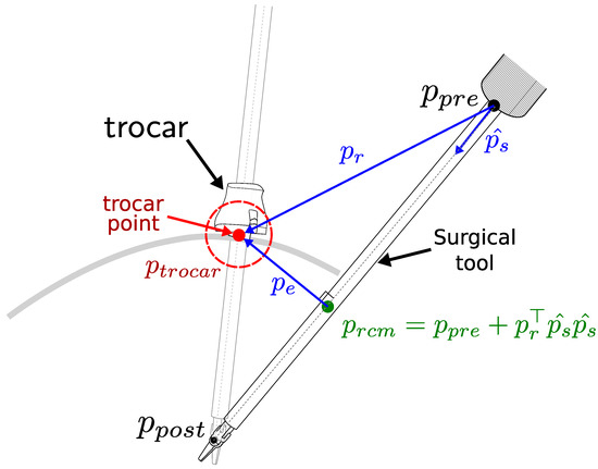
Figure 1.
Characterization of the remote center of motion (RCM). The motion of the surgical tool is constrained by the trocar point, resulting in an RCM error, which is defined as the minimum distance between the tool axis and the trocar point .
By differentiating with respect to the manipulator joints , the RCM constraint task Jacobian matrix can be calculated as
with
where and are the configuration-dependent analytical Jacobian matrices of the immediate joints before and after RCM, respectively.
The residual of the RCM constraint task is defined as the minimum distance to the trocar point and can be calculated as
The Jacobian representation of the RCM constraint and the residual of the RCM task are then used for the hierarchical constraint IK formulation.
3.1.2. Tool Tip Pose Control Task
For a tool tip pose control task, we define the actual and desired end-effector pose as the transformations and of the robot end-effector frame with respect to an inertial frame B, respectively.
The task Jacobian matrix is defined by
The 6D pose task residual is defined by
where the logarithm maps the pose from the Lie group to twists in the [38].
3.2. Inverse Jacobian IK Solver
Classical inverse kinematics, based on inverse Jacobian methods, is widely used for its simplicity and fast computation. It is based on the differential kinematics formulation . in which is the task space vector, q is the manipulator’s joint vector, and is the configuration-dependent task Jacobian matrix relating joint velocities with task space velocities. Given a desired task space velocity , the inverse kinematic problem is defined as finding a suitable , such as
The least-squares solution for this problem can be obtained using the Moore–Penrose pseudoinverse of , defined as
where , and P denotes the orthogonal projection operator in the null space of J, while z is an arbitrary task velocity vector that does not disturb task and can be used for secondary tasks.
Given k tasks with different priorities, a hierarchy between tasks is enforced by recursively solving the inverse kinematic problem for each task in the null space of the previous ones. A recursive formula is given by [25]
with , and represents the projector in the null space of the augmented Jacobian .
For our inverse Jacobian IK solver, two tasks were considered: an RCM constraint task and a tool tip pose control as a secondary task. The desired joint velocities are given by
Here, and denote the Jacobians of the RCM and the end-effector tasks, respectively. and are the desired task velocities for the RCM constraint and tool tip pose tracking tasks, respectively. The tool pose control task has a lower priority and is solved in the null space of the RCM constraint task. A closed-loop inverse kinematics (CLIK) version of this equation is usually implemented as [24]
Inverse Jacobian methods are often unable to handle inequality constraints, such as joint limits, which can limit their effectiveness in certain applications. A common solution is to truncate the solutions within the joint limits range, but this approach does not guarantee that the algorithm will not get stuck within the joint limit region. To address this issue, we propose a random restart strategy, which involves restarting the algorithm from a new, randomly chosen starting joint configuration if a solution is found outside of the joint range. This approach ensures that the algorithm will continue to search for a solution while also staying within the bounds of the joint limits, ultimately improving its effectiveness and efficiency in constrained inverse kinematics problems.
3.3. Nonlinear Optimization IK Solver
The inverse Jacobian approach cannot explicitly handle inequality constraints and is susceptible to convergence failure when closed to the joint limits or local minima. The constrained inverse kinematics problem can be redefined with a nonlinear soft restricted optimization formulation, where a weight is assigned to each ith task according to its priority. A general optimization problem for constrained IK with k tasks is given by
where and denote additional equality and inequality constraints for the IK problem. For the proposed nonlinear optimization IK solver, the RCM constraint task and the tool pose control task are given a weight coefficient and respectively, with . The optimization problem is defined as
where and are the lower and upper joint limits, respectively, and represents a control cycle period. The last term works as a regularizer, whereas the inequality constraint avoids exceeding the joint limits.
3.4. Hierarchical Quadratic Programming IK Solver
The general inverse kinematics problem in (7) of each task can be represented as a general least squares problem given by
with being the optimization variable. , , and are arbitrary matrices, , , arbitrary vectors, is the ith task dimension, and and are dimensions of the equality and inequality constraints, respectively.
Each least squares representation of the task can be solved as a quadratic programming (QP) problem hierarchically by ensuring the optimality condition between successive tasks , following the approach proposed by Kanoun et al. [39]. The higher priority tasks are protected from the influence of lower priority tasks by incorporation of the null-space projector operator in the optimization formulation, which ensures that the lower priority tasks are executed in the null space of the previous tasks.
For our HQP IK solver, the RCM constraint task with joint limits inequality constraint is defined as
By adding convenient slack variables , inequality constraints can be transformed into
The QP formulation of the RCM task constraint for the optimization variable is represented as
with , , , and , are defined as
where , , and .
The tool pose control task is defined in a similar way considering the solution for the RCM constraint task and the null-space projector as
The QP formulation is given by
with , , defined as
where , , and
3.5. Concurrent IK Solvers
Concurrent IK solvers combine individual IK solvers and offer a trade-off between their capabilities. Our implementation includes four concurrent IK solvers: INVJ+NLO, INVJ+HQP, HQP+NLO, and INVJ+NLO+HPP. INVJ and HQP solvers follow strict prioritization, while NLO uses a non-strict hierarchy with weighted objectives based on task priority.
Synchronization between solvers is performed via multi-threading, and mutex lock is ensured before writing in shared memory. Each solver has an enable flag, and the solver will search for a solution as long as the flag is activated. Multiple concurrency strategies can be followed to choose an IK solution from multiple solvers. A possible strategy could be to wait for a predefined time, and if multiple solutions are provided, choose the one that meets a selection criterion (e.g., manipulability maximization). We use a time prioritization strategy to select the best IK solution. As soon as one solver finds a solution, it will attempt to stop the other solvers. However, due to checking the enable flag only at the start of a new iteration, this may not be immediate. For optimization-based solvers like HQP and NLO, stopping is not possible during optimization execution, and a longer stopping time may occur. For NLO, we set a minimum of five iterations before checking the enable flag to avoid the time cost of leaving after one optimization iteration to check the enable flag and then restart the search.
3.6. IK Solvers Implementation
In this study, the IK solvers were implemented in C++ on a Linux Ubuntu 20.04 workstation with an Intel Core i9-11900 processor and 64 GB of RAM. The implementation was designed to be compatible with the robotics operating system (ROS) framework. For kinematic computations, transformations, and kinematic chain parsing, we employed the Pinocchio library (v. 2.6.10) [40]. We used CASadi (v. 3.5.5) [41] as a backend for nonlinear and HQP solvers, using IPOPT (v. 3.14.5) [42] with HSL/MA57 linear solver for nonlinear optimization and OSQP (v. 0.5.0) [43] for quadratic programming in the HQP solver, both with warm start enabled. The proposed implementation is used in both the simulation and the real-world experimental validations presented in Section 4 and Section 5, respectively.
4. Numerical Evaluation Based on Simulation
The performance evaluation of the proposed method was initially carried out in a simulation environment. The evaluation metrics considered were: solve rate, average solving time, and RCM deviation.
4.1. Simulation Environment
A simulation environment was developed in Coppeliasim [44] to evaluate the performance of various inverse kinematics solvers in redundant kinematic chains commonly found in RMIS applications, where endoscopes and surgical tools are frequently used. We considered three different kinematic chains, shown in Figure 2:
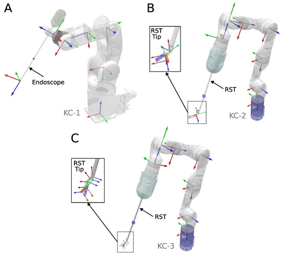
Figure 2.
Three kinematic chains were used for numerical validation in simulation. (A) A 6-DOF endoscope holder. (B) A 7-DOF manipulator holding a 3-DOF robotic surgical tool. (C) A 7-DOF manipulator holding a 5-DOF robotic surgical tool.
- KC-1: A 6-DOF Robot manipulator (Denso VS-050) with a rigid endoscope attached.
- KC-2: A 7-DOF Robot manipulator (Kinova Gen3) with a 3-DOF robotic surgical tool (OpenRST [45]) attached. One degree of freedom is dedicated to opening and closing the gripper and is not considered for IK solving.
- KC-3: A 7-DOF Robot Manipulator (Kinova Gen3) with a 5-DOF robotic hyper-redundant surgical tool attached. One degree of freedom is dedicated to opening and closing the gripper, and is not considered for IK solving.
4.2. Unconstrained Inverse Kinematics Benchmark
To assess the performance of concurrent IK solvers, we first considered an unconstrained scenario (i.e., no RCM restriction), and conducted a benchmark against established IK libraries used in robotic applications, namely Orocos KDL and Trac-IK [20], which are widely adopted to solve unconstrained IK problems. We randomly generated 10,000 target poses by running forward kinematics on random joint configurations, ensuring that at least one solution exists. The parameters used for the unconstrained benchmark are presented in Table 1.

Table 1.
Parameters used for the unconstrained inverse kinematics benchmark.
Table 2 summarizes the IK solve rate and the average computation time for successful solutions with the three kinematic chains.
Table 2.
A comparison of solve rate and solving time for a total of nine IK solvers: five single-method and four concurrent. The targets are randomly selected from reachable poses. Evaluation is performed for three kinematic chains commonly found in robot-assisted surgical applications: KC-1 (Endoscope Holder), KC-2 (Manipulator + OpenRST), and KC-3 (Manipulator + Hyper-redundant RST). The highest values in each column are highlighted in bold.
Figure 3 presents a comparison of computation times for the tested IK solvers. Orocos KDL, an inverse Jacobian solver with a truncated joint limits strategy, showed the lowest solve rate among all the IK solvers due to frequently getting stuck in local minima. On the contrary, TRAC-IK, which combines an inverse Jacobian IK solver and a sequential quadratic programming solver using a concurrent strategy, showed a high solve rate of 99.8% and an average computation time of 0.462 ms. However, INVJ and INV+HQP outperformed TRAC-IK, achieving similar solve rates with shorter computation times of 0.187 and 0.190 ms, respectively. The inverse Jacobian method with random restarts proved effective, even for highly redundant kinematic chains. HQP+INVJ takes the most advantage of the INVJ solver, achieving a short stopping time and performance similar to INVJ. NLO+INVJ also showed a significant improvement in the solve rate and computation time but was still far from INVJ and INVJ+HQP. The worst time performance is found in the INVJ+NLO+HQP solver, which is likely due to conflicts in shared resources among the three individual solvers. NLO and HQP solvers faced challenges in finding solutions, with an average solve rate of 80% and 78%, respectively. Since they are based on local optimizers, they are sensitive to initial guesses, and with the definition of random targets, the time to find a solution sometimes exceeds the timeout set at 10 ms.
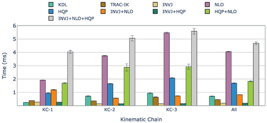
Figure 3.
Average solving time (ms) of successful IK solves with unconstrained random targets for each kinematic chain and IK implementation. Considering all evaluated kinematic chains, INVJ and INVJ+HQP showed the best performance, with solving times of less than 0.2 ms.
4.3. Constrained Inverse Kinematics Benchmark
We conducted a benchmark to compare the performance of inverse kinematics (IK) solvers with the remote center of motion (RCM) constraint. We defined the targets as two 6D tracking paths along circumferences of 3 cm and 10 cm, respectively. Each target path is divided into 100 trajectory steps. In contrast to the unconstrained random benchmark scenario, we do not use Orocos-KDL and TRAC-IK due to their inability to handle additional constraints. The concurrent solvers INVJ+NLO+HQP and HQP+NLO showed poorer performance than their concurrent counterparts on the unconstrained benchmark and were not included in this experiment. The parameters used in the constrained benchmark are listed in Table 3.
Table 3.
Parameters used for the constrained inverse kinematics benchmark.
Since the KC-1 kinematic chain only has six DOFs, it is not possible to track a 6DOF path, and a 4DOF path is chosen, with the target endoscope roll angle fixed. Snapshots of the KC-1 path tracking are shown in Figure 4. The solve rate and the solving time are summarized in Table 4.
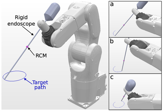
Figure 4.
Simulation environment for KC-1 (endoscope holder) tracking a 10 cm circular path. The trajectory followed by the endoscope tip is visualized in blue, and snapshots (a–c), shown on the right, depict the robot executing the tracking task at different trajectory steps.
Table 4.
A comparison of the solve rate and the solving time for single-method and concurrent IK algorithms. The target trajectories are two circular paths with diameters of 3 cm and 10 cm. Evaluation is performed for the KC-1 kinematic chain (endoscope holder).
Except for NLO, all the IK solvers evaluated achieved a perfect solve rate of 100%. The computation times for each case are shown in Figure 5. The optimization-based single IK solvers, NLO and HQP, showed the worst performance with computation times of approximately 0.720 ms and 0.510 ms, respectively. However, INVJ and INVJ-based concurrent IK solvers exhibited superior performance with an average computation time of around 0.060 ms.
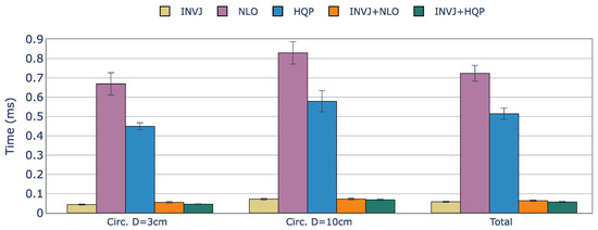
Figure 5.
Average runtime (ms) of successful IK solves for a constrained tracking task with KC-1 (endoscope holder) kinematic chain. The best time performance is achieved by the INVJ-based IK solvers with average solving times of 0.07 ms.
The KC-2 kinematic chain has a total of ten DOFs (seven DOFs from the manipulator and three DOFs from the surgical tool). A 6-DOF path is defined with the tip of the surgical tool pointing downward throughout the task, as shown in Figure 6. Table 5 summarizes the solve rate and solving time performance.
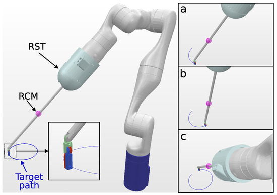
Figure 6.
Simulation environment for KC-2 Kinematic chain (OpenRST) tracking a 10 cm circular path. In the close-up view, the tool tip target orientation is shown. The trajectory followed by the surgical tool tip is visualized in blue, and snapshots (a–c), shown on the right, depict the robot executing the tracking task at different trajectory steps.
Table 5.
A comparison of the solve rate and the solving time for single-method and concurrent IK algorithms. The target trajectories are two circular paths with diameters of 3 cm and 10 cm. Evaluation is performed for the KC-2 (Manipulator + OpenRST) kinematic chain.
The solve rate for the INVJ solver drops dramatically for this kinematic chain with a solve rate of less than 50% in both cases and an average computation time of approximately 6 ms, as shown in Figure 7. Concurrent solvers rely on optimization-based solvers to achieve a solve rate of 100%. The computation time is higher for the HQP-based solvers, with an average of 2.4 ms, in contrast to the average of 1.9 ms obtained for the NLO-based solvers.
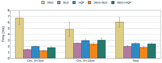
Figure 7.
Average runtime (ms) of successful IK solves for a constrained tracking task with KC-2 (OpenRST) kinematic chain. The concurrent solvers demonstrated slightly better performance than their respective optimization-based single-method IK solvers, with INVJ showing the worst time performance due to its low solve rate.
The KC-3 kinematic chain has a total of 12 DOFs (seven DOFs from the manipulator and five DOFs from the surgical tool) and represents a case in which a highly redundant surgical tool is used. The 6-DOF path considers a target orientation for the tip of the surgical tool that points upward throughout the task, as shown in Figure 8.
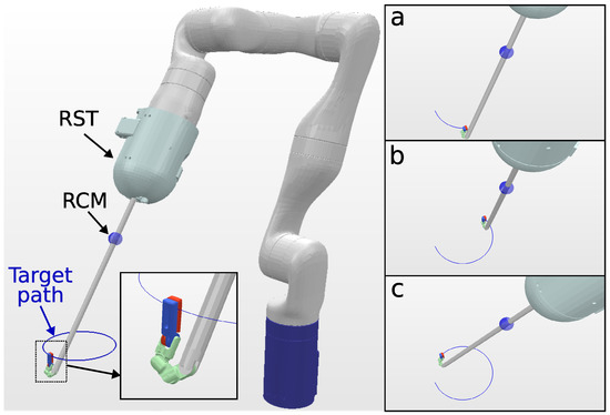
Figure 8.
Simulation environment for KC-3 Kinematic chain (Hyper-redundant RST) tracking a 10 cm circular path. In the close-up view, the tool tip target orientation. The trajectory followed by the surgical tool tip is visualized in blue, and snapshots (a–c), shown on the right, depict the robot executing the tracking task at different trajectory steps.
The solve rate and the average computation time are shown in Table 6. Although the basic INVJ solver exhibited a low solve rate, its concurrent versions that combined it with optimization-based solvers were able to achieve high solve rates. In general, the results of the average computation time indicate that the concurrent IK solvers, INVJ+NLO and INVJ+HQP, performed the best with average computation times of 1.58 and 1.54 ms, respectively, as illustrated in Figure 9.
Table 6.
A comparison of the solve rate and the solving time for single-method and concurrent IK algorithms. The target trajectories are two circular paths with diameters of 3 cm and 10 cm. Evaluation is performed for the KC-3 kinematic chain (Manipulator + Hyper-redundant RST).
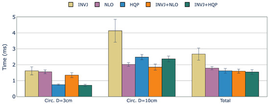
Figure 9.
Average runtime (ms) of successful IK solves for a constrained tracking task with KC-3 (Hyper-redundant RST) kinematic chain. The concurrent solvers demonstrated slightly better performance than their respective optimization-based single-method IK solvers, with INVJ+HQP showing the best average solving time performance.
4.4. Summary of the Results in Simulation
Numerical evaluation based on simulation compared the performance of the proposed concurrent IK solvers in constrained and unconstrained scenarios. For the unconstrained scenario, the results showed an important difference in performance between the IK solvers based on the Inverse Jacobian and optimizers, with TRAC-IK and the solvers based on INVJ (INVJ, INVJ+NLO and INVJ+HCP) showing a high success ratio of about 100% for all evaluated kinematic chains. However, INVJ and INVJ+HQP showed better time performance than TRACK-IK, with average solving times of less than 0.2 ms.
In the constrained scenario (i.e., the RCM constraint enabled), INVJ-based IK solvers exhibited superior performance with an average computation time of around 0.05 ms for the KC-1 kinematic chain, which represents a basic endoscope holder case. For more complex scenarios, such as the KC-2 kinematic chain that involves a surgical tool and the KC-3 kinematic chain that involves a highly redundant surgical tool, the basic INVJ solver exhibited a low solve rate. However, its concurrent versions that combined it with optimization-based solvers were able to achieve high solve rates of about 100%. When considering all kinematic chains and target paths, summarized in Table 7, INVJ performs poorly, with a solve rate of 72% and the longest average computation time. On the other hand, optimization-based IK solvers exhibit better performance with HQP achieving an average solve rate of 99%. Additionally, NLO significantly reduces pose and RCM errors compared to other solvers, as it continuously searches for the optimal solution until convergence and only stops to check the enable flag after five iterations. On average, the concurrent IK solvers, INVJ+NLO and INVJ+HQP, deliver superior performance in terms of solve rate and computation time, with INVJ+NLO exhibiting the best computation time.
Table 7.
A comparison of solve rate and time performance for single and concurrent IK algorithms considering all target paths.
5. Real-World Experiments for RMIS Scenarios
The proposed constrained IK solvers were validated through real-world experiments for two path-tracking tasks that closely resemble RMIS scenarios: robot-assisted endoscope positioning and robotic surgical tool pose control. Given the poor performance of INVJ in constrained IK problems, this experiment focused solely on evaluating the single IK solvers NLO and HQP, as well as the concurrent IK solvers INV+NLO and INVJ+HQP. The parameters used are the same as those given in Table 3.
5.1. Robot-Assisted Endoscope Positioning
The robotic system is shown in Figure 10A, which consists of a 6-DOF manipulator (VS-050, Denso Robotics, Long Beach, CA, USA) and a rigid endoscope mounted on its end effector. The tracking target is a 4-DOF path, with the translation path defined as a helix of 5 cm diameter described by
with and . The trajectory was divided into 750 steps. The additional DOF orientation constraint is defined as the roll angle equal to , so the endoscope image does not rotate while translating.
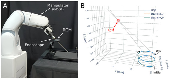
Figure 10.
Endoscope positioning experiment (A) Experimental setup. A 6-DOF manipulator (VS 050, Denso Corp.) with a rigid endoscope mounted. (B) The RCM constraint and the helix trajectory followed for each IK solver.
A motion capture system (Optitrack, Corvallis, OR, USA) is utilized to capture the endoscope’s position by placing markers on the endoscope shaft. The trajectory followed by the endoscope tip is depicted in Figure 10B. The solve rate and the average computation time are summarized in Table 8.
Table 8.
Solve rate and solving time performance for a 6-DOF robotic endoscope holder tracking a 4D helix path (D = 5 cm).
The NLO solver had the lowest solve rate at 8% and a computational time of 3.3 ms, as shown in Figure 11A. The HQP solver was able to achieve a 100% solve rate with an average computational time of 1.3 ms. However, the concurrent IK solvers, which include the INVJ solver, were able to provide solutions in less than 0.2 ms, demonstrating an 85% improvement over the HQP solver. The INV+HQP solver exhibited the best performance, achieving a 100% solve rate and an average RCM error of 0.42 mm. Visualization of the changes in the RCM error throughout the trajectory can be observed in Figure 11B. Due to its low solve rate, the NLO solver was unable to accurately track the desired endoscope trajectory.
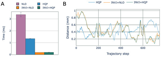
Figure 11.
(A) Average IK solving time for the endoscope positioning task. (B) RCM error for each IK solver obtained from motion capture for each step of the helix trajectory.
Snapshots of the trajectory followed by the manipulator are shown in Figure 12.
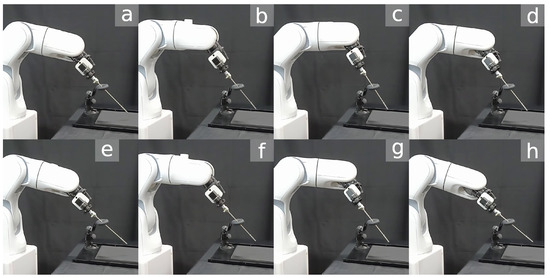
Figure 12.
Snapshots of a robotic endoscope holder tracking a 4-DOF helix path subjected to an RCM constraint. The labels (a–h) indicate the sequence of the robot’s movement along the path.
5.2. Multi-DOF Robotic Surgical Tool Pose Control
The implemented IK solvers were also evaluated for a pose control task of a multi-DOF surgical tool. The robotic system, shown in Figure 13A, comprises a 7-DOF robotic manipulator (Gen3, Kinova) with a 3-DOF robotic surgical tool (Fenestrated OpenRST [45]) attached to its end effector. The target path is a 6-DOF Lissajous curve , where the translation path is defined by
with , , , and . The trajectory is divided into 2500 steps . The target orientation is fixed on a predefined rotation matrix , which corresponds to pointing toward the right side of the image in Figure 13. Markers are attached to the tool shaft to record deviations from the RCM constraint. The trajectory followed is shown in Figure 13B.
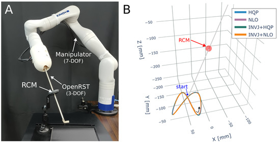
Figure 13.
Endoscope positioning experiment (A) A 7-DOF manipulator (Gen3, Kinova) with a 3-DOF robotic surgical tool attached to the end effector. (B) The RCM constraint and the Lissajous trajectory followed for each IK solver.
The solve rate and the average solving time for all IK solvers are summarized in Table 9. All solvers were able to complete the task with a solve rate of approximately 100%. The NLO solver had the longest solving time, with an average of 4.4 ms, as shown in Figure 14A. Concurrent IK solvers demonstrated faster solving times, with INVJ+HQP performing the best with an average solving time of 2.7 ms. The average RCM error was less than 1 mm for all solvers, with maximum deviations of up to 1.9 mm for INVJ+NLO and 1.7 mm for INVJ+HQP, as shown in Figure 14B. Snapshots of the followed trajectory are shown in Figure 15.
Table 9.
Solve rate and solving time performance for a 7-DOF robotic manipulator + 3 DOF RST tracking a 6D Lissajous path.
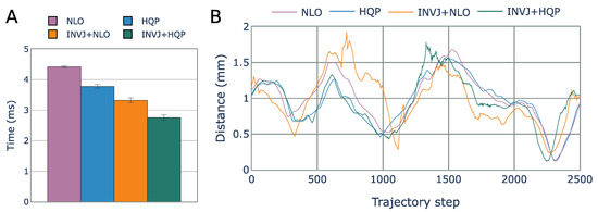
Figure 14.
(A) Average IK solving time for the surgical tool pose control task. (B) RCM error for each IK solver obtained from motion capture for each step of the Lissajous trajectory.

Figure 15.
Snapshots of the robotic surgical tool tracking a 6-DOF Lissajous path subjected to an RCM constraint. The labels (a–h) indicate the sequence of the robot’s movement along the path.
6. Conclusions
In this study, we proposed a novel framework that addresses the challenging constrained inverse kinematics problem in robot-assisted minimally invasive surgery (RMIS), where the RCM constraint is a fundamental requirement. The proposed framework combines classical inverse Jacobian IK and optimization-based IK approaches into a concurrent IK solver. Specifically, we combined the inverse Jacobian (INVJ) method with hierarchical quadratic programming (HQP) and nonlinear optimization (NLO) solving strategies to explicitly incorporate RCM constraints and joint limits into the optimization process. To further enhance IK solving performance, we proposed a concurrent multithreaded deployment of IK solvers.
We evaluated the proposed method through experimental validation in simulation for common kinematic chains found in RMIS applications in both unconstrained and constrained scenarios. Our results indicated that the INVJ solver showed high performance in unconstrained scenarios, but its performance deteriorated in constrained cases. In contrast, optimization-based IK solvers exhibited good performance for constrained tasks and low performance for the unconstrained task. The concurrent IK solvers proposed that include both methods (INVJ+NLO and INVJ+HQP) exhibited good performance in both tasks. We validated their performance in real-world experiments, consisting of an endoscope positioning task and a pose control task with a robotic surgical tool. Our experiments demonstrated that both concurrent IK solvers showed a significant improvement over single-method IK solvers, ensuring a 100% solve rate and reducing the solving time up to 85% for the endoscope positioning task and 37% for the pose control of a multi-dof robotic surgical tool. In particular, INVJ+HQP showed the highest solve rate and the lowest computation time in real-world experiments. On the other hand, optimization-based single IK solvers, NLO and HQP, showed the worst performance with higher computation times. Therefore, it may be beneficial to use concurrent IK solvers that combine optimization-based and iterative-based solvers for improved performance.
However, the real-world performance of concurrent inverse kinematics (IK) solvers depends on the availability of computational resources. In particular, the use of multithreading may limit their implementation on embedded hardware with a limited number of processors and memory resources. When implementing the proposed framework, it is important to consider critical aspects of managing concurrency, such as resource sharing and synchronization, to avoid race conditions or data corruption. Additionally, debugging concurrent IK solvers can be more difficult due to their non-deterministic behavior. To further facilitate the development and evaluation of the proposed framework, we provide open access to the IK solvers implemented in this study.
One of the challenges of our proposed method is the potential for sudden changes in joint acceleration when transitioning between different inverse kinematics (IK) solvers. These changes can lead to unwanted jerky motion, which may negatively impact the performance of the system. An additional limitation is the limited number of constraints considered for the IK problem, only including joint limits and the RCM restriction. To address these issues, future work will focus on analyzing these transitions and developing strategies to mitigate their effects, and incorporating additional constraints, such as collision avoidance or manipulability maximization, to further enhance the performance of the proposed framework. Although general IK solvers are suitable for covering a broad range of robotic platforms, they may not ensure optimal performance. Therefore, parameter tuning may be necessary to achieve better performance for specific hardware. Automated parameter optimization is another potential avenue for improving the proposed framework.
In general, this work presents a novel and effective solution to the constrained IK problem in RMIS applications, with the potential for broader applications in robotics and automation.
Author Contributions
Conceptualization, J.C.; methodology, J.C.; software, J.C., and A.D.; experiments, J.C., A.D. and K.F.; writing—original draft preparation, J.C. and A.D.; writing—review and editing, Y.H.; supervision, Y.H.; project administration, Y.H.; funding acquisition, Y.H. All authors have read and agreed to the published version of the manuscript.
Funding
This work was supported in part by the Japan Science and Technology Agency (JST) CREST including AIP Challenge Program under Grant JPMJCR20D5, and in part by the Japan Society for the Promotion of Science (JSPS) Grants-in-Aid for Scientific Research (KAKENHI) under Grant 22K14221.
Institutional Review Board Statement
Not applicable.
Informed Consent Statement
Not applicable.
Data Availability Statement
The implementation code of this work is openly available at https://github.com/jcolan/CoIKS (accessed on 19 March 2023).
Conflicts of Interest
The authors declare no conflict of interest.
Abbreviations
The following abbreviations are used in this manuscript:
| MIS | Minimally invasive surgery |
| RMIS | Robot-assisted minimally invasive surgery |
| DOF | Degree of freedom |
| IK | Inverse kinematics |
| RST | Robotic surgical tool |
References
- Colan, J.; Davila, A.; Hasegawa, Y. A Review on Tactile Displays for Conventional Laparoscopic Surgery. Surgeries 2022, 3, 334–346. [Google Scholar] [CrossRef]
- Guthart, G.S.; Salisbury, J.K. The Intuitive telesurgery system: Overview and application. In Proceedings of the 2000 IEEE International Conference on Robots and Automation (ICRA), San Francisco, CA, USA, 24–28 April 2000; pp. 618–621. [Google Scholar] [CrossRef]
- D’Ettorre, C.; Mariani, A.; Stilli, A.; Rodriguez y Baena, F.; Valdastri, P.; Deguet, A.; Kazanzides, P.; Taylor, R.H.; Fischer, G.S.; DiMaio, S.P.; et al. Accelerating Surgical Robotics Research: A Review of 10 Years with the da Vinci Research Kit. IEEE Robot. Autom. Mag. 2021, 28, 56–78. [Google Scholar] [CrossRef]
- Koyama, Y.; Marinho, M.M.; Mitsuishi, M.; Harada, K. Autonomous Coordinated Control of the Light Guide for Positioning in Vitreoretinal Surgery. IEEE Trans. Med. Robot. Bionics 2022, 4, 156–171. [Google Scholar] [CrossRef]
- Colan, J.; Nakanishi, J.; Aoyama, T.; Hasegawa, Y. A Cooperative Human-Robot Interface for Constrained Manipulation in Robot-Assisted Endonasal Surgery. Appl. Sci. 2020, 10, 4809. [Google Scholar] [CrossRef]
- Marinho, M.M.; Harada, K.; Deie, K.; Ishimaru, T.; Mitsuishi, M. SmartArm: Suturing Feasibility of a Surgical Robotic System on a Neonatal Chest Model. IEEE Trans. Med Robot. Bionics 2021, 3, 253–256. [Google Scholar] [CrossRef]
- Chen, Y.; Zhang, S.; Wu, Z.; Yang, B.; Luo, Q.; Xu, K. Review of surgical robotic systems for keyhole and endoscopic procedures: State of the art and perspectives. Front. Med. 2020, 14, 382–403. [Google Scholar] [CrossRef]
- Yaşır, A.; Kiper, G.; Dede, M.C. Kinematic design of a non-parasitic 2R1T parallel mechanism with remote center of motion to be used in minimally invasive surgery applications. Mech. Mach. Theory 2020, 153, 104013. [Google Scholar] [CrossRef]
- Kuo, C.H.; Dai, J.S.; Dasgupta, P. Kinematic design considerations for minimally invasive surgical robots: An overview. Int. J. Med Robot. Comput. Assist. Surg. 2012, 8, 127–145. [Google Scholar] [CrossRef]
- Freschi, C.; Ferrari, V.; Melfi, F.; Ferrari, M.; Mosca, F.; Cuschieri, A. Technical review of the da Vinci surgical telemanipulator. Int. J. Med Robot. Comput. Assist. Surg. 2013, 9, 396–406. [Google Scholar] [CrossRef]
- Hagn, U.; Konietschke, R.; Tobergte, A.; Nickl, M.; Jörg, S.; Kübler, B.; Passig, G.; Gröger, M.; Fröhlich, F.; Seibold, U.; et al. DLR MiroSurge: A versatile system for research in endoscopic telesurgery. Int. J. Comput. Assist. Radiol. Surg. 2010, 5, 183–193. [Google Scholar] [CrossRef]
- Moe, S.; Antonelli, G.; Teel, A.R.; Pettersen, K.Y.; Schrimpf, J. Set-Based Tasks within the Singularity-Robust Multiple Task-Priority Inverse Kinematics Framework: General Formulation, Stability Analysis, and Experimental Results. Front. Robot. AI 2016, 3, 16. [Google Scholar] [CrossRef]
- Mannucci, A.; Caporale, D.; Pallottino, L. On Null Space-Based Inverse Kinematics Techniques for Fleet Management: Toward Time-Varying Task Activation. IEEE Trans. Robot. 2021, 37, 257–274. [Google Scholar] [CrossRef]
- Mansard, N.; Khatib, O.; Kheddar, A. A Unified Approach to Integrate Unilateral Constraints in the Stack of Tasks. IEEE Trans. Robot. 2009, 25, 670–685. [Google Scholar] [CrossRef]
- Dufour, K.; Suleiman, W. On maximizing manipulability index while solving a kinematics task. J. Intell. Robot. Syst. 2020, 100, 3–13. [Google Scholar] [CrossRef]
- Chiacchio, P.; Chiaverini, S.; Sciavicco, L.; Siciliano, B. Closed-Loop Inverse Kinematics Schemes for Constrained Redundant Manipulators with Task Space Augmentation and Task Priority Strategy. Int. J. Robot. Res. 1991, 10, 410–425. [Google Scholar] [CrossRef]
- Berenson, D.; Srinivasa, S.; Kuffner, J. Task Space Regions: A framework for pose-constrained manipulation planning. Int. J. Robot. Res. 2011, 30, 1435–1460. [Google Scholar] [CrossRef]
- Diankov, R. Automated Construction of Robotic Manipulation Programs. Ph.D. Thesis, Carnegie Mellon University, Pittsburgh, PA, USA, 2010. [Google Scholar]
- Escande, A.; Mansard, N.; Wieber, P.B. Fast resolution of hierarchized inverse kinematics with inequality constraints. In Proceedings of the 2010 IEEE International Conference on Robotics and Automation, Anchorage, AK, USA, 3–7 May 2010; pp. 3733–3738. [Google Scholar] [CrossRef]
- Beeson, P.; Ames, B. TRAC-IK: An open-source library for improved solving of generic inverse kinematics. In Proceedings of the 2015 IEEE-RAS 15th International Conference on Humanoid Robots, Seoul, Republic of Korea, 3–5 November 2015; pp. 928–935. [Google Scholar] [CrossRef]
- Dai, H.; Izatt, G.; Tedrake, R. Global inverse kinematics via mixed-integer convex optimization. Int. J. Robot. Res. 2019, 38, 1420–1441. [Google Scholar] [CrossRef]
- An, S.i.; Lee, D. Prioritized Inverse Kinematics: Generalization. IEEE Robot. Autom. Lett. 2019, 4, 3537–3544. [Google Scholar] [CrossRef]
- Siciliano, B.; Slotine, J.J. A general framework for managing multiple tasks in highly redundant robotic systems. In Proceedings of the Fifth International Conference on Advanced Robotics ’Robots in Unstructured Environments, Pisa, Italy, 19–22 June 1991; Volume 2, pp. 1211–1216. [Google Scholar] [CrossRef]
- Chiaverini, S. Singularity-robust task-priority redundancy resolution for real-time kinematic control of robot manipulators. IEEE Trans. Robot. Autom. 1997, 13, 398–410. [Google Scholar] [CrossRef]
- Mansard, N.; Chaumette, F. Task Sequencing for High-Level Sensor-Based Control. IEEE Trans. Robot. 2007, 23, 60–72. [Google Scholar] [CrossRef]
- Escande, A.; Mansard, N.; Wieber, P.B. Hierarchical quadratic programming: Fast online humanoid-robot motion generation. Int. J. Robot. Res. 2014, 33, 1006–1028. [Google Scholar] [CrossRef]
- Gholami, S.; Tassi, F.; De Momi, E.; Ajoudani, A. A Reconfigurable Interface for Ergonomic and Dynamic Tele-Locomanipulation. In Proceedings of the 2021 IEEE/RSJ International Conference on Intelligent Robots and Systems (IROS), Prague, Czech Republic, 27 September–1 October 2021; pp. 4260–4267. [Google Scholar] [CrossRef]
- Tassi, F.; De Momi, E.; Ajoudani, A. Augmented Hierarchical Quadratic Programming for Adaptive Compliance Robot Control. In Proceedings of the 2021 IEEE International Conference on Robotics and Automation (ICRA), Xi’an, China, 30 May–5 June 2021; pp. 3568–3574. [Google Scholar] [CrossRef]
- Azimian, H.; Patel, R.V.; Naish, M.D. On constrained manipulation in robotics-assisted minimally invasive surgery. In Proceedings of the 2010 3rd IEEE RAS & EMBS International Conference on Biomedical Robotics and Biomechatronics, Tokyo, Japan, 26–29 September 2010; pp. 650–655. [Google Scholar] [CrossRef]
- Aghakhani, N.; Geravand, M.; Shahriari, N.; Vendittelli, M.; Oriolo, G. Task control with remote center of motion constraint for minimally invasive robotic surgery. In Proceedings of the 2013 IEEE International Conference on Robotics and Automation, Karlsruhe, Germany, 6–10 May 2013; pp. 5807–5812. [Google Scholar] [CrossRef]
- Marinho, M.M.; Harada, K.; Mitsuishi, M. Comparison of remote center-of-motion generation algorithms. In Proceedings of the 2017 IEEE/SICE International Symposium on System Integration (SII), Taipei, Taiwan, 11–14 December 2017; pp. 668–673. [Google Scholar] [CrossRef]
- Sandoval, J.; Poisson, G.; Vieyres, P. A new kinematic formulation of the RCM constraint for redundant torque-controlled robots. In Proceedings of the 2017 IEEE/RSJ International Conference on Intelligent Robots and Systems (IROS), Vancouver, BC, Canada, 24–28 September 2017; pp. 4576–4581. [Google Scholar] [CrossRef]
- Osa, T.; Staub, C.; Knoll, A. Framework of Automatic Robot Surgery System using Visual Servoing. In Proceedings of the 2010 IEEE/RSJ International Conference on Intelligent Robots and Systems, Taipei, Taiwan, 18–22 October 2010; pp. 1837–1842. [Google Scholar] [CrossRef]
- Marinho, M.M.; Bernardes, M.C.; Bo, A.P.L. Using General-Purpose Serial-Link Manipulators for Laparoscopic Surgery with Moving Remote Center of Motion. J. Med Robot. Res. 2016, 1, 1650007. [Google Scholar] [CrossRef]
- Kapoor, A.; Li, M.; Taylor, R. Constrained control for surgical assistant robots. In Proceedings of the 2006 IEEE International Conference on Robotics and Automation, ICRA 2006, Orlando, FL, USA, 15–19 May 2006; pp. 231–236. [Google Scholar] [CrossRef]
- Yang, S.; Wang, Y.; Zhao, H.; Cheng, H.; Ding, H. Autonomous Laparoscope Control for Minimally Invasive Surgery With Intuition and RCM Constraints. IEEE Robot. Autom. Lett. 2022, 7, 7934–7941. [Google Scholar] [CrossRef]
- Colan, J.; Nakanishi, J.; Aoyama, T.; Hasegawa, Y. Optimization-Based Constrained Trajectory Generation for Robot-Assisted Stitching in Endonasal Surgery. Robotics 2021, 10, 27. [Google Scholar] [CrossRef]
- Solà, J.; Deray, J.; Atchuthan, D. A micro Lie theory for state estimation in robotics. arXiv 2018, arXiv:1812.01537. [Google Scholar]
- Kanoun, O.; Lamiraux, F.; Wieber, P.B. Kinematic Control of Redundant Manipulators: Generalizing the Task-Priority Framework to Inequality Task. IEEE Trans. Robot. 2011, 27, 785–792. [Google Scholar] [CrossRef]
- Carpentier, J.; Saurel, G.; Buondonno, G.; Mirabel, J.; Lamiraux, F.; Stasse, O.; Mansard, N. The Pinocchio C++ library: A fast and flexible implementation of rigid body dynamics algorithms and their analytical derivatives. In Proceedings of the 2019 IEEE/SICE International Symposium on System Integration (SII), Paris, France, 14–16 January 2019; pp. 614–619. [Google Scholar] [CrossRef]
- Andersson, J.A.; Gillis, J.; Horn, G.; Rawlings, J.B.; Diehl, M. CasADi: A software framework for nonlinear optimization and optimal control. Math. Program. Comput. 2019, 11, 1–36. [Google Scholar] [CrossRef]
- Wächter, A.; Biegler, L.T. On the implementation of an interior-point filter line-search algorithm for large-scale nonlinear programming. Math. Program. 2006, 106, 25–57. [Google Scholar] [CrossRef]
- Stellato, B.; Banjac, G.; Goulart, P.; Bemporad, A.; Boyd, S. OSQP: An operator splitting solver for quadratic programs. Math. Program. Comput. 2020, 12, 637–672. [Google Scholar] [CrossRef]
- Rohmer, E.; Singh, S.P.N.; Freese, M. V-REP: A versatile and scalable robot simulation framework. In Proceedings of the 2013 IEEE/RSJ International Conference on Intelligent Robots and Systems, Tokyo, Japan, 3–7 November 2013; pp. 1321–1326. [Google Scholar] [CrossRef]
- Colan, J.; Davila, A.; Zhu, Y.; Aoyama, T.; Hasegawa, Y. OpenRST: An Open Platform for Customizable 3D Printed Cable-Driven Robotic Surgical Tools. IEEE Access 2023, 11, 6092–6105. [Google Scholar] [CrossRef]


Disclaimer/Publisher’s Note: The statements, opinions and data contained in all publications are solely those of the individual author(s) and contributor(s) and not of MDPI and/or the editor(s). MDPI and/or the editor(s) disclaim responsibility for any injury to people or property resulting from any ideas, methods, instructions or products referred to in the content. |
© 2023 by the authors. Licensee MDPI, Basel, Switzerland. This article is an open access article distributed under the terms and conditions of the Creative Commons Attribution (CC BY) license (https://creativecommons.org/licenses/by/4.0/).