Article

A Fault-Detection System Approach for the Optimization of Warship Equipment Replacement Parts Based on Operation Parameters

by
Álvaro Michelena
1,*,†,
Víctor López
1,*,†,
Francisco Lamas López
2,3,
Elena Arce
1,
José Mendoza García
2,4,
Andrés Suárez-García
5,
Guillermo García Espinosa
2,4,
José-Luis Calvo-Rolle
1,* and
Héctor Quintián
1
1
Department of Industrial Engineering, University of A Coruña (UDC), CTC, CITIC, Rúa Mendizábal, s/n, 15403 Ferrol, Spain
2
Centro de Supervisión y Análisis de Datos de la Armada (CESADAR), Arsenal de Cartagena, Armada Calle Real s/n, 30290 Cartagena, Spain
3
Computing and Artificial Intelligence Laboratory (CAILab), Facultad de Ciencia y Tecnología, Universidad Camilo José Cela, Calle Castillo de Alarcón 49, 28692 Madrid, Spain
4
Área de Sostenimiento y Gestión Logística, ISDEFE, Calle Beatriz de Bobadilla, 3., 28040 Madrid, Spain
5
Spanish Naval School, University Defense Center, 36920 Marín, Spain
*
Authors to whom correspondence should be addressed.
These authors contributed equally to this work.
Sensors 2023, 23(7), 3389; https://doi.org/10.3390/s23073389
Submission received: 27 January 2023 / Revised: 11 March 2023 / Accepted: 20 March 2023 / Published: 23 March 2023
(This article belongs to the Special Issue Feature Papers in Fault Diagnosis & Sensors Section 2022)

Abstract

:
Systems engineering plays a key role in the naval sector, focusing on how to design, integrate, and manage complex systems throughout their life cycle; it is therefore difficult to conceive functional warships without it. To this end, specialized information systems for logistical support and the sustainability of material solutions are essential to ensure proper provisioning and to know the operational status of the frigate. However, based on an architecture composed of a set of logistics applications, this information system may require highly qualified operators with a deep knowledge of the behavior of onboard systems to manage it properly. In this regard, failure detection systems have been postulated as one of the main cutting-edge methods to address the challenge, employing intelligent techniques for observing anomalies in the normal behavior of systems without the need for expert knowledge. In this paper, the study is concerned to the scope of the Spanish navy, where a complex information system structure is responsible for ensuring the correct maintenance and provisioning of the vessels. In such context, we hereby suggest a comparison between different one-class techniques, such as statistical models, geometric boundaries, or dimensional reduction to face anomaly detection in specific subsystems of a warship, with the prospect of applying it to the whole ship.

1. Introduction

Among many benefits, there are two significant cross-cutting advantages in ship automation: the crew diminution and the hazards and risks reduction of the people in general and the ship itself [1]. The first implies a significant reduction in ship operating costs directly [2]. Indirectly, it would entail aspects related to improving the conditions of workers in general terms (training, social security, the possibility of oversizing the workforce, …) [3]. On the second way, remark that in general terms, automation confers advantages with reducing risks for workers since it is the automatic machine that performs the work and the worker normally reduces his work to supervision. In addition, tedious and repetitive tasks, with the problems that these entails, are carried out by automata [3].
From a technical point of view, automation implies optimization if the accomplishing is correct [4]. In this sense, if the ship processes are well automated, then as result, advantages such as emissions reduction, consumption reduction, increased reliability, and availability could be achieved. Consequently, aspects as important as sustainability and reduction of environmental impact would be favored [5]. These aspects must continue to be pursued and improved as technology advances, and as there is a margin within which to do so.
The current convulsed geopolitical situation invites us to pay special attention to the military sector.Given the evolution of today’s societies, losing lives in armed conflicts is tremendously unpopular from a country’s political point of view [6]. Because of all this, it is a priority right now to put the minimum number of human lives at risk. It is especially important to try to move towards solutions similar to those of unmanned aerial vehicles (UAVs) or functional robots. The government’s goal is to achieve zero human deaths in the face of any military intervention [6].
In the specific case of warships, all the ship aspects mentioned before are applicable. However, it is necessary to consider and add the characteristics and conditions of military ships. In addition to multiple singularities, this kind of ship usually has more confined and optimized spaces [7]. Due to these characteristics, it would be desirable for this type of ship to transport only the essentials, and of course to guarantee satisfactory operation.
In general terms, the ships have a certain useful life. The same thing happens with warships, and it is even more restrictive. The fact that the useful life is shorter will depend, among others, on the economy of the country, of popularity from a social point of view, and on obsolescence from a military point of view [8]. Operationally, ships should ideally be at the forefront of technology.
Like in other sectors, the design of the warships obviously depends on the current technology and its future trend. Nowadays, as in the industry, there is a very strong trend in the naval sector towards digitization [9]. From an operational point of view, warships tend to install this type of technology because of the advantages they bring [10]. Thanks to this kind of relatively incipient technology, the optimization possibilities on ships are huge compared to the current state. It is necessary to emphasize that due to issues such as climate change or global warming, it is also mandatory that everything is carried out from a point of view of sustainability, energy efficiency, and low emissions.
Anomaly or failure detection is one of the objectives that must be achieved in any sector [11]. Digitization allows and helps carrying out this kind of technique, even giving new advantages from a reliability and accuracy point of view [12]. If this task is carried out satisfactorily, new advantages can be achieved in operation. Some of them are, for example, the increase in the efficiency of maintenance tasks, shipment of the optimal number of spare parts, or the optimization of the material purchase process.
There are many anomaly detection methods [13,14]. Consequently, there are several possible classifications that can be made of the types of existing techniques [13]. In some cases, an exhaustive knowledge of the system on which failure detection is intended is necessary [15]. This fact can have certain advantages during the process, such as better results, accuracy, and/or performance [12]. However, in cases where operating personnel change frequently, it can be very important that exhaustive process knowledge is not necessary [12]. Thus, they could perform anomaly detection autonomously or with non-expert operators.
Anomaly detection in several ships’ systems is essential in order to know the operational status of the frigate. Therefore, analyzing and detecting anomalies or malfunctions is a previous and necessary step to predict the possible spare parts to be shipped depending on the ship’s condition.
This research paper deals with a novel fault detection system approach applied to certain onboard subsystems, aiming to expand to the entire ship. In this manner, our proposal tests a set of different intelligent techniques following a one-class conceptualization, where only information from the system’s normal operation is consumed to model its performance during the training stage.
The present research work is organized as follows. After the current introduction, the related works are described. After this section, the case of the study is explained, detailing the equipment and the information system structure. Then, the materials and the methods taken into account for the present research are detailed. The work is continued with a description of the experiments and their results. Finally, conclusions and future works are presented.

2. Related Work

Throughout this section, we briefly mention recent work that may be related to the present study, either according to the techniques employed or the application to warship equipment.
Many reviews are oriented toward maintenance practices and strategies. In this sense, Kimera et al. [16] provide an overview of the maintenance parameters and practices that are critical for marine mechanical systems classified as plant, machinery, and equipment (PME). Previously, Cullum et al. [17] focused on the risk-based maintenance (RBM) scheduling framework as applied to warships and naval vessels, and provided a critical analysis of the risk assessment and maintenance scheduling techniques in use. More recently, Zhang et al. [18] reviewed the methods, strategies, and application of marine systems and equipment (MSAE) in prognostics and health management (PHM) as an essential means to optimize resource allocation and improve the intelligent operation and maintenance (O&M) efficiency of MSAE.
Along these lines, in relation to the PHM of naval mechanical systems, there are other works from the perspective of technical processes. For example, online condition monitoring and self-repair techniques for in-service marine diesel engines [19], different types of blade failures and current blade failure-detection methods [20], and mainly data-driven models and the problem of condition-based maintenance of marine propulsion systems are reviewed [21]. In the field of autonomous shipping, Karatug et al. [22] propose an evaluation of PHM systems and reliability centered maintenance strategies, as one method that can be implemented to cover the three major elements of maintenance management systems: risk assessment, maintenance strategy selection, and maintenance task interval, according to Emovon et al. [23] for autonomous marine vessels.
For its part, considering the current status and future trends of maintenance strategies applied in particular to corroded marine steel structures, Abbas et al. [24] analyzed deterministic and probabilistic models for predicting corrosion rates.
Other works propose their own strategies, suggesting a predictive maintenance solution based on a computational artificial intelligence model using real-time monitoring data, as stated by Jimenez et al. [25]. They also expose a ship-level method for repair decisions based on the preventive maintenance concept, relying on an improved failure mode and effects analysis (FMEA) method along with a Weibull distribution model, where the parameters are intended to be calculated using the maximum likelihood estimation (MLE) to predict the characteristic life of the equipment, and then determine the actions to be taken regarding logical decision principles and rule-based reasoning (RBR) in agreement with Song et al. [26].
A short time ago, in search of tackling decision making problems, Emovon et al. [27] presented a comparison of hybrid multi-criteria decision making (MCDM) methods for the selection of appropriate maintenance strategies for ship machinery systems and other related ship systems. Similarly, employing dynamic condition monitoring and historic data to present decision support information onboard, Michala et al. [28] proposed a novel decision support system (DSS) beforehand. Lately, making use of subjective opinions in DSS, Maurice et al. [29] attempted a technique for order preference by similarity to an ideal situation for ranking the maintenance strategies. Prior studies have proven that a decision support mechanism needs multiple criteria decision on ship equipment maintenance strategy selection [30,31,32].
With the specific aim of minimizing maintenance costs and maximizing ship reliability simultaneously, Zhao et al. [33] tested whether a bi-objective model under a condition-based maintenance strategy was applicable to the point of being able to provide support for ship operators.
In the arena of machine learning (ML) and especially fault detection systems, quite a few works can be found in the literature. Studies alike employ several prediction techniques, including regularized linear regression methods such as L1 (lasso) and L2 (ridge), or long short-term memory (LSTM)-based networks [34]. In this context, previous research has used artificial neuronal networks (ANN) [35] and decision trees [36], as well as support vector machines (SVM) [37,38] or the k-nearest neighbor technique (k-NN) as one of the most common for fault classification [39]. Moreover, in this scope, various deep learning (DL) techniques have also been used, as in the case of autoencoder neural networks [40] or recurrent neural networks (RNN) [41] based on long short-term memory network (LSTM) cells according to Yang et al. [42].
Some of the latest research achievements on the DL-based state of health prognostic methods address issues with limited labeled samples without assuming that the training and test datasets come from identical machines operating under similar conditions. In this context, Zhu et al. [43] developed Bayesian semi-supervised transfer learning with an active querying-based intelligent fault prognostic framework for remaining useful life (RUL) prediction across completely different machines under limited data.
As a compilation of the state of the art, recent reviews presented developments within fault detection and diagnosis (FDD) methods [44], introduced a survey of trends and techniques of fault detection in networked dynamical systems (NDS) [45], and gave an overview the theory and strategies of transient fault detection [46].
Other review papers lead to a specific field of application, as may be the optimal performance of photovoltaic (PV) systems [47,48], uninterrupted and trouble-free operation of induction motors (IMs) [49] or transient stability in a transmission network in agreement with Mishra et al. [50].
Working on novel approaches, some studies are available within the industrial processes area, proposing a fault detection system based on intelligent techniques [51,52]. In addition, certain previous works particularly focused on alternatives to hardware-only and software-only systems, as mentioned by Reis et al. [53] who identifed hybrid hardware/software fault-detection mechanisms.
To conclude, several references based on the techniques that stand the anomaly detection approach in the current study are present in the bibliography and discussed in more detail across Section 4.

3. Case of Study

This section introduces the technical–administrative processes, as far as the study is concerned, through which logistical support and sustainability considerations of material solutions are integrated into the navy as we know it today, specifically for the Spanish. The context in which the project takes place and where all the data monitoring and management is performed by the Data Supervision and Analysis Center of the Spanish Navy (CESADAR).

3.1. Equipment

Generally speaking, warships are very expensive systems, extraordinarily complex, with a lengthy procurement acquisition process and long operational life. During their life cycle, their configuration changes as a result of repairs and modifications. Therefore, the objective of integrated logistics support (ILS) [54] is to maximize system availability by optimizing the life cycle cost and ensuring mission compliance.
Another essential process is logistics configuration (LC), also referred to as the configuration, which encompasses the logistics processes required for thedevelopment of the ILS during the life cycle, defining the systems, subsystems, equipment, and components installed, with a description of their functional, physical and technical characteristics, quantity, type, and number of modifications made to each of them, as well as all available supporting documentation, recorded in documents and databases.
Following a functional criterion, the configuration is represented by a AEC (configured elements tree) that has a hierarchical structure. In the AEC, each element is assigned a HSC (hierarchical structure code) that works as a functional marking, up to 12 digits, which makes it possible to identify and distinguish that element univocally from others. Thereby, this HSC code is used as a reference in efforts such as the maintenance processes, spare parts management, etc.
By way of example, Figure 1 depicts how the AEC is developed on the basis of the operational requirements, identifying the functional nodes in accordance with the navy’s material guidelines, which defines the levels of hierarchical decomposition for assigning the functional mark of an element in the AEC.
Thereby, in order to control the evolution of onboard equipment, systems engineering has as its most effective tool the configuration management (CM) system, which provides an overview of the system development. At the same time, it is also an indispensable aspect for achieving interoperability, mitigating risks, and making effective use of NATO (The North Atlantic Treaty Organization) capabilities [56] in joint operations.
For the achievement of CM, the Spanish navy, through CESADAR, is supported by information and communication technologies (ICT) using a range of logistics applications which are itemized in the following subsection.

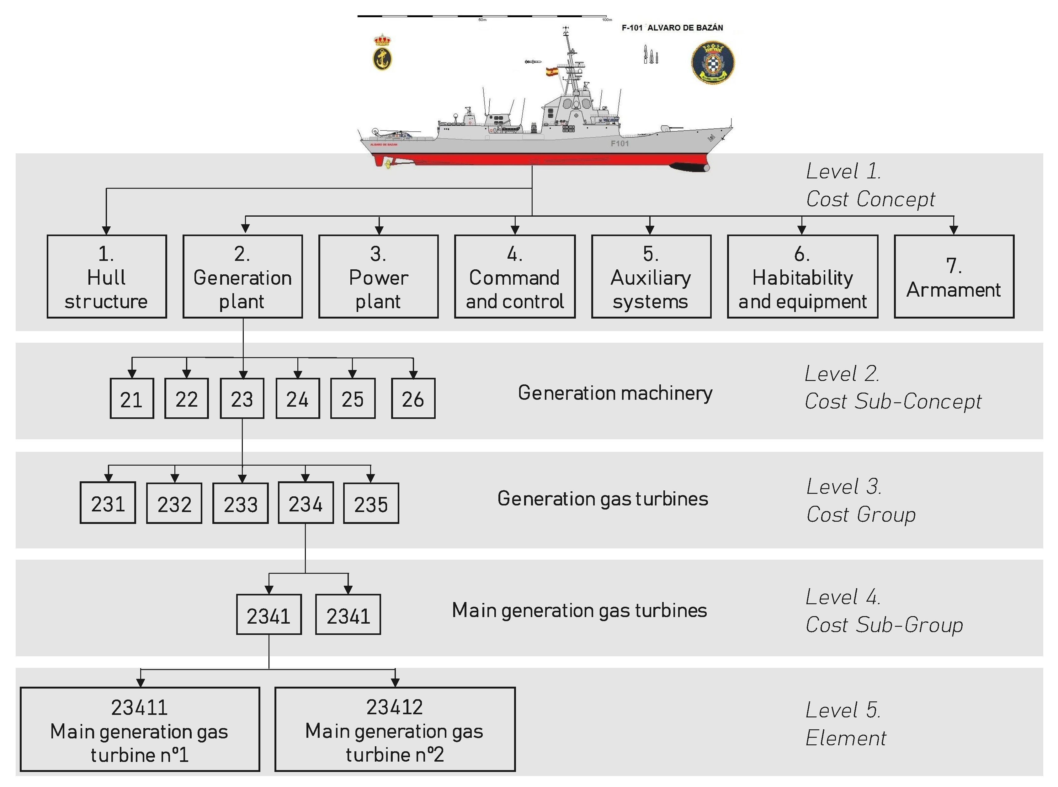
3.2. Warship Information System Structure

With participation in a multitude of missions since their commissioning in 2002, mainly under the NATO umbrella, the Spanish Álvaro de Bazán class frigates (F-100) were appointed to the investigation. Playing the role of the main source of information, CESADAR is the centralized system in charge of receiving, checking, and analyzing the data recorded in the vessels, and which in turn is stored and structured within its data lake.
Up until now, CESADAR has as one of its main applications the automation of surveillance and analysis tasks logistics application (ATAVIA), which provide a system for detecting anomalies in the operation of the monitored equipment based on expert rules. Indeed, all sensorized onboard systems and equipment are analyzed.
In addition to these, several separate applications developed in different programming languages and databases have been employed so far for logistics management, mainly from maintenance and procurement, posing a considerably complex architecture [55].
These logistics applications are difficult systems that require in-depth knowledge and expert analysis. Likewise, some authors have reviewed these tools proposing an alternative semi-unsupervised predictive maintenance system [34]. From our side, we focus on a novel fault detection system approach based on operational data provided by the ATAVIA application, as discussed below.

4. Materials and Methods

This section describes the techniques considered to achieve anomaly detection. The datasets used are also presented.

4.1. Employed Methods

The proposal follows a one-class approach, in which only information from the normal operation of the system is used to model its performance. Then, the detection of anomalous situations must be addressed without prior knowledge of their nature.
According to the literature [57], the implementation of one-class techniques can be based on three different principles: dimensional reduction techniques, statistical models, and the determination of geometric boundaries. To assess the performance of these three different approaches, four different techniques are proposed to model the normal behavior of the ship to detect anomalies.

4.1.1. Statistical Models

An interesting approach to face anomaly detection using one-class techniques is based on the idea of using density functions. One commonly used statistical model is tested in this work.

Gaussian Model

One of the most direct ways to achieve a one-class classifier consists of applying a Gaussian distribution function over the training set, also known as a target set [57]. The covariance matrix and the mean vector are calculated and then a new test value is labeled depending on the score achieved at the Gaussian function.
Let us suppose a test instance x R n , whose distribution probability function is described in Equation (1). The function would produce lower values if x is not part of the target class. Therefore, selecting an appropriate threshold value would enable correct classification.
p ( x , μ , Σ ) = 1 ( 2 π ) n / 2 Σ 1 / 2 e 1 2 ( x μ ) T Σ 1 ( x μ )
where:
  • μ is the training set mean value;
  • Σ is the training set covariance matrix.
This simple idea is characterized by a low computational cost, with the calculation of the covariance matrix being the most challenging step. Incorporating a regularization parameter R p can be a valuable tool, particularly in cases where the inverse of the covariance cannot be computed.
Although this method demonstrates excellent performance, particularly when the target set is normally distributed [58], it does share a limitation with other density estimation techniques: the requirement for a sufficiently large training dataset [59].

4.1.2. Geometric Boundaries

The calculation of the geometric boundaries of the target set can represent a good approximation to determine the difference between expected and unexpected events.

K-Means

The k-means unsupervised algorithm represents an intuitive way to achieve a one-class classifier, depending on the geometric distribution of the data [60].
After selecting the desired number of groups, the k-means algorithm partitions a given dataset into k clusters by minimizing the objective function expressed in Equation (2).
e = k = 1 C x ϵ ϱ k x c k 2
where:
  • x represents a new input vector;
  • c k denotes the centroid of the k cluster.
The centroids for each group are calculated using the training set to use k-means as a one-class technique. The distance of a given test data point to its closest centroid is then compared to the distances between each cluster data point and its respective centroid. The test data point is classified as anomalous if the distance exceeds all such distances.
For example, Figure 2 illustrates a case where the training set is divided into two clusters. In this instance, the black dot, representing a test point, is classified as a target because its distance to the nearest centroid (the orange star of Cluster 2) is lower than the distances of most training samples.

4.1.3. Dimensional Reduction

The last one-class approach consists of the application of dimensional reduction techniques to learn patterns that only are presented in the target set.

Autoencoder

Utilizing artificial neural networks (ANN) configured with an autoencoder design in dimensional reduction techniques has produced substantial favorable outcomes [61].
To this end, the multilayer perceptron (MLP), which is one of the most common ANN architectures, is implemented. The MLP typically comprises an input layer, an output layer, and one or more hidden layers. The neurons in the contiguous layers are connected by weighted links that are automatically adjusted to minimize the discrepancy between the produced output and the desired output. Each layer also possesses an activation function applied to all the neurons within that layer, such as the linear, step, tan-sigmoid, or log-sigmoid function. The hidden layer output is computed using Equation (3),
h i = f 1 ( W 1 x i + b 1 )
where:
  • h i defines the output of the hidden layer;
  • f 1 is the hidden layer activation function;
  • W 1 corresponds to the weight matrix between input and hidden layer;
  • x i is the input vector;
  • b 1 denotes the bias vector.
Subsequently, the output of the ANN is obtained using Equation (4).
x ^ = f o ( W o h i + p o )
where:
  • x ^ is the ANN output.
  • f o denotes the activation function of the output layer.
  • W o define the weight matrix between hidden and output layers.
  • p o is the bias vector.
The fundamental principle of the autoencoder involves training an ANN so that the output x ^ is equal to the input x while also executing a nonlinear reduction within the hidden layer through the activation function. This means that the number of neurons in the hidden layer must be lower than that of the inputs, which results in decompression being performed at the output [61]. The autoencoder method operates on the premise that anomalous points are significantly different from standard points in the hidden layer subspace, and the decompression process leads to high reconstruction errors.

Principal Component Analysis

Principal component analysis (PCA) is a commonly used technique for data dimensionality reduction tasks. This technique aims to identify the directions in the data with the highest variability and use them to establish new variables [60,62]. These directions are referred to as components and are calculated using the eigenvectors obtained from the eigenvalues of the covariance matrix.
PCA projects the original data points into the eigenvectors subspace, resulting in linear transformations. This technique is particularly effective in cases where the subspace is clearly linear.
In addition to its performance in dimensional reduction tasks, PCA can also be applied to one-class problems using reconstruction error criteria. For instance, suppose we have a training set X R 2 and use one of the two principal components to linearly transform it into X ^ R 1 . A test data point x t is labeled based on a reconstruction error criteria (Equation (5)), calculated as the difference between the initial point x t and its projection x t ^ .
Anomalous points are likely to have higher reconstruction errors, and hence when the reconstruction error of a test data point is above a specific threshold, the anomaly is detected.
e ( x ) = | | x t x ^ t | |
An instance where the distance from a test point to its projection exceeds all distances from the training points to their respective projections is illustrated in Figure 3. In this scenario, only the first component is utilized. The threshold distinguishing normal from anomalous behavior is frequently associated with the percentile distance of the training set.

4.2. Dataset

The information available through the abovementioned application, ATAVIA, has been used to obtain the working datasets. This application includes sensorization, warnings, and alarms of malfunctioning systems and equipment. For the present research, different subsystems of the vessels were selected as the object of analysis, selecting diesel power generation equipment. Specifically, three different datasets corresponding to the operation of a different components of the diesel generator have been used. No information about the study component and dataset features is provided for confidentiality reasons. In addition, generic names will be used to refer to them.
The working datasets contain the information captured by the sensors associated with each component within a 1 min period (sample rate of 0.016667 Hz), as well as the target variable, which indicates whether the sample corresponds to the normal or anomalous system performance. The operating data are available from May 2011 to May 2022.
It is important to emphasize that in this research only data recorded with the diesel generator operating in a stationary regime have been used, since the fault detection system from which the data are obtained generates a large number of false alarms in the system start-up and shutdown processes, minimizing the dataset quality.
Finally, the three working datasets are:
  • Dataset 1 contains two variables and a total of 902,796 samples, of which 219 correspond to anomalous data.
  • Dataset 2 contains two variables and 897,191 samples, of which 101 correspond to anomalous data.
  • Dataset 3 contains twenty-five variables and 887,294 samples, of which 233 correspond to anomalous data.

5. Experiments Description (Setup) and Results

The research presented in this paper discusses the performance of three alternative one-class approaches. For this purpose, four different techniques are evaluated to model the normal performance of selected components of the power-generation system of the F-100 frigates. To obtain the best performance of each technique, several experiments have been carried out.

5.1. Experimental Setup and Assessment

To validate and compare the proposed techniques, different experiments have been carried out for each of the three datasets mentioned in Section 4.2. To achieve the best classifier, the performance of each technique has been evaluated for different values of its hyperparameters. The evaluated configurations are listed below.
  • Gaussian Model
    Data normalization
    Data regularization
    Outlier factor
  • K-means
    Data normalization
    Number of clusters
    Outlier factor
  • Autoencoder
    Data normalization
    Neurons in the hidden layer
    Outlier factor
  • Principal Component Analysis
    Data normalization
    Number of components considered
    Outlier factor
Each technique has been evaluated for three different data conditions. First, the data were used without any normalization process, NoNorm, then the data were normalized using a 0 to 1 criterion, Norm, and finally, the z-score method was applied (with a mean of 0 and a standard deviation of 1), Zscore [63]. The use of these normalization techniques, Zscore, in combination with one-class classification methods, has shown satisfactory results [64].
Moreover, each technique has been tested with different percentages of outliers in the training dataset. Values of 0, 5, 10, and 15% were used. The different configurations that have been tested for each technique are summarized in Table 1. All the one-class techniques have been implemented in Matlab R2022b using different packages and toolboxes.
Finally, it is important to highlight that k-fold cross-validation with a k = 3 was used for model validation and training. A schematic of the experimental setup is shown in Figure 4.

5.2. Results

The classifier performance evaluation has been measured using the area under the receiver operating curve (AUC) metric. This metric is well known in classifier performance analysis, and its result, measured as a percentage, relates false positive and true positive rates. In addition, the AUC is commonly used in cases where the dataset is unbalanced, as it is insensitive to class imbalance. Since the k-fold cross-validation method is used, the AUC results correspond to the mean performance of each configuration. In this way, each classifier’s training time has been considered to evaluate the computational cost. As a matter of fact, the results obtained for the different configurations of each technique are shown in Table 2, Table 3, Table 4, Table 5, Table 6 and Table 7.
Table 2 collects the results for the different configurations evaluated with the Gaussian model. As shown, in the three datasets the best AUC scores are registered with the data without normalization, with a regularization value of 0.009 and an outlier factor of 5% (in dataset 1 and 2) and 15% (in dataset 3). With this particular combination, with the first dataset, an AUC of 95.797% was obtained, 97.592% with the second data set, and 86.222% with the high-dimensional dataset.
In general terms, it can be observed that the Gaussian model is a technique with a low computational cost. In fact, none of the tested configurations exceeded a training time of 0.01 s for both datasets with two features, and for the third dataset, most settings had training times of less than 1 s.
Similarly, the resolution for the different sets of parameters evaluated with the k-means technique are summarized in Table 3. In this case, other combinations provide better performance for each dataset. As depicted, with dataset 1, the most favorable outcomes are obtained with a total of 2 clusters, an outlier factor of 10%, and normalizing the data with the z-score method; achieving with this specific configuration a 95.075% AUC. On the other hand, in the second experiment, with dataset 2, a percentage of 97.544% AUC was scored with the 6-cluster classifier implemented with an outlier factor of 5%, and the data normalized with the 0/1 criterion. Finally, the best classifier for the third dataset is obtained with 4 clusters, an outlier factor of 10%, and a Zscore normalization. With this configuration, an AUC value of 91.539% is achieved.
Generally speaking, with the k-means technique, good efficiency is appreciated with a fairly low computational cost. Still, analyzing Table 3, it is noticeable how the classifiers with an outlier factor of 0% do not achieve beneficial values. This fact can be produced as a consequence of possible anomalies labeled as normal data.
As before, Table 4 and Table 5 introduce the findings validated with PCA. Table 4 shows the results for the first two datasets of 2 variables, while Table 5 shows the performance of PCA with the dataset of 25 variables. It is important to note that Table 5 only offers the best configurations obtained by selecting each of the different numbers of the components since if all the tested configurations were shown, the table would contain a large amount of information that may compromise its comprehensibility.
In this case, analyzing Table 4, the most effective design is similar for both datasets since the best behavior is displayed with one component and the data normalized with the 0/1 criterion. The difference in the configurations corresponds to the percentage of the outlier factor. Firstly, through simulation with dataset 1, the highest AUC value, 88%, is collected with an outlier factor of 15%, while in the second case, the best classifier, with 97% of AUC, has been built considering 5% of outliers in the training set.
On the other hand, Table 5 demonstrates the effectiveness of PCA for high-dimensional data sets (data set 3). The best outcomes are obtained by normalizing the data by the 0/1 criterion, using an outlier factor of 5% of the training set, and selecting only 1 or 2 components. Following this approach, classifiers with AUC values above 90% can be achieved. However, using many components does not yield favorable results with this technique.
In general, it is worth noting that the computational cost of PCA is also quite low. None of the tested configurations exceeded training times of 0.6 s for the two-variable datasets, while for the 25-variable dataset, the average training times were approximately 3 s.
Finally, Table 6 and Table 7 present the solutions found with the autoencoder neural network. As with the PCA technique, the results are shown in two different tables. In addition, due to the large number of features of the third dataset, it is important to note that Table 7 only shows the best configurations for the different numbers of neurons tested.
For this method, the finest outcomes also depend on different internal computations. In the case of the first dataset (Table 6), using 1 neuron in the network hidden layer, an outlier factor of 15%, and the 0/1 normalization method; it ends with an 87.6% AUC. Nevertheless, with the second dataset (Table 6), the most promising values are attained considering 5% of the training data as outliers and also with 0/1 data normalization. Indeed, reaching up to more than 97% AUC.
On the other hand, by analyzing Table 7, it can be appreciated how the autoencoder neural networks are also capable of achieving good results in warship components with a large number of associated variables. In this case, with the third dataset, this technique reached more than 90% AUC using only 2 neurons in the hidden layer and considering a 5% outlier factor and a normalization of the data following the 0/1 criterion. However, for this dataset, it can be observed that with the increase in the number of neurons in the hidden layer, the performance is not good, and the tested classifiers do not achieve values higher than 70% AUC.
Although the results obtained in terms of AUC have been quite good with the three datasets, the computational cost of this technique is considerable, taking its toll with training times exceeding 4000 s.
Figure 5 provides a bar chart comparison of the performance of each implemented one-class technique with its respective dataset. The results are highly satisfactory, with AUC values exceeding 90%. Based on the results obtained for each technique and dataset, along with their computational costs, the k-means approach emerges as the most suitable method as it yields the highest average AUC value across all datasets analyzed.

6. Conclusions and Future Works

The present study has focused on the use of one-class techniques for anomaly detection in different components of a warship diesel generator. For this purpose, the performance of four one-class methods has been compared, using three different datasets corresponding to the data collected on the Spanish Navy F-100 frigates between May 2011 and May 2022.
Analyzing the achievements, it has been possible to prove that satisfactory results have been obtained in the different datasets with the four compared techniques. In the first experiment performed, with dataset 1, more than 95% AUC was recorded with the Gaussian model and k-means, while the autoencoder neural network and the PCA technique had worse performance. In the second case, dataset 2, all the implemented techniques give more than 97% AUC. Finally, with the third dataset, classifiers with an AUC higher than 90% have been achieved for all techniques except the Gaussian model.
Considering the computational cost, it has been shown that the Gaussian model, k-means, and PCA have very low rates. Moreover, the training stage of the autoencoder classifiers involves a much higher computational cost than the aforementioned techniques. In this case, the training time depends directly on the number of features of the dataset and the data normalization, given that the largest values are registered without this feature.
In general terms, this research has shown that one-class techniques are capable of detecting anomalies in the vessel component under analysis. This is a great improvement compared to the anomaly detection systems currently in operation on the ship, since their management requires very detailed knowledge of their individual functionalities of each component. Therefore, designing and tuning the current anomaly detection systems requires a large amount of expert man-hours to ensure a good performance in detecting possible failures. In addition, due to the different dynamics of the various components of a warship, a different design is required for each of these components which is an arduous task of design and adjustment.
However, with the proposal presented in this paper, the use of one-class techniques can simplify the design of these failure detection systems in diesel generator components of a warship, since no expert knowledge of the system is required. In addition, design and adjustment times could be drastically reduced, saving many thousands of Euros in commissioning these services.
On the other hand, this paper has demonstrated that one-class techniques can be used with high performance in different ship components, so the proposal’s flexibility, integration, and scalability are assured, being able to use these algorithms in other subsystems of the vessel.
In future work, the performance of these techniques on other ship components may be analyzed with the aim of obtaining a standardized approach that can detect anomalies in any component of the diesel generator. Accordingly, due to the different components within the vessel, the possibility of using hybrid classifiers based on combining clustering techniques with one-class algorithms may also be studied. In this way, more robust classifiers that could detect anomalies in various ship components would be developed. On the other hand, another line of future research will be the analysis of the anomalies detected by the proposed system in order to facilitate the management of the necessary shippable spare parts.

Author Contributions

Methodology, Á.M. and V.L.; Investigation, Á.M., V.L., F.L.L., E.A., J.M.G., A.S.-G., G.G.E., J.-L.C.-R. and H.Q.; Writing—original draft, Á.M., V.L., J.-L.C.-R. and H.Q.; Writing—review & editing, Á.M., V.L., J.-L.C.-R. and H.Q.; Supervision, J.-L.C.-R. and H.Q.; Funding acquisition, F.L.L., E.A., J.M.G. and G.G.E. All authors have read and agreed to the published version of the manuscript.

Funding

This research received no external funding.

Institutional Review Board Statement

Not applicable.

Informed Consent Statement

Not applicable.

Acknowledgments

Álvaro Michelena’s research was supported by the Spanish Ministry of Universities (https://www.universidades.gob.es/ (accessed on 21 March 2023)), under the “Formación de Profesorado Universitario” grant with reference FPU21/00932. CITIC, as a Research Center of the University System of Galicia, is funded by Consellería de Educación, Universidade e Formación Profesional of the Xunta de Galicia through the European Regional Development Fund (ERDF) and the Secretaría Xeral de Universidades (Ref. ED431G 2019/01). We thank the Spanish Navy for supporting this investigation. We also thank Isdefe (Ingeniería de Sistemas para la Defensa de España) for sponsoring it.

Conflicts of Interest

The authors declare no conflict of interest.

References

  1. Khastgir, S.; Birrell, S.; Dhadyalla, G.; Sivencrona, H.; Jennings, P. Towards increased reliability by objectification of Hazard Analysis and Risk Assessment (HARA) of automated automotive systems. Saf. Sci. 2017, 99, 166–177. [Google Scholar] [CrossRef]
  2. Wahidi, S.; Pribadi, S.; Pribadi, T.; Wardhana, N.; Arif, M. Fixed Manpower Reduction Analysis to Reduce Indirect Cost of Ship Production. In Proceedings of the 5th International Conference on Marine Technology (SENTA 2020), Surabaya, Indonesia, 8 December 2020; IOP Publishing: Bristol, UK, 2021; Volume 1052, p. 012048. [Google Scholar]
  3. Hannaford, E.; Hassel, E.V. Risks and Benefits of Crew Reduction and/or Removal with Increased Automation on the Ship Operator: A Licensed Deck Officer’s Perspective. Appl. Sci. 2021, 11, 3569. [Google Scholar] [CrossRef]
  4. Manis, K.; Madhavaram, S. AI-Enabled marketing capabilities and the hierarchy of capabilities: Conceptualization, proposition development, and research avenues. J. Bus. Res. 2023, 157, 113485. [Google Scholar] [CrossRef]
  5. Ang, J.H.; Goh, C.; Saldivar, A.A.F.; Li, Y. Energy-efficient through-life smart design, manufacturing and operation of ships in an industry 4.0 environment. Energies 2017, 10, 610. [Google Scholar] [CrossRef]
  6. Thompson, J.H. An Unpopular War: From Afkak to Bosbefok; Penguin Random House: Saxonwold, South Africa, 2011. [Google Scholar]
  7. La Monaca, U.; Bertagna, S.; Marinò, A.; Bucci, V. Integrated ship design: An innovative methodological approach enabled by new generation computer tools. Int. J. Interact. Des. Manuf. (IJIDeM) 2020, 14, 59–76. [Google Scholar] [CrossRef]
  8. Xing, T.; Song, B.; Ye, J.; Zhao, Z. General Analysis Method of Warship Service Life. In Proceedings of the 2010 Second WRI Global Congress on Intelligent Systems, Wuhan, China, 16–17 December 2010; IEEE: Piscataway, NJ, USA, 2010; Volume 3, pp. 223–228. [Google Scholar]
  9. Stanić, V.; Hadjina, M.; Fafandjel, N.; Matulja, T. Toward shipbuilding 4.0-an industry 4.0 changing the face of the shipbuilding industry. Brodogr. Teor. Praksa Brodogr. Pomor. Teh. 2018, 69, 111–128. [Google Scholar] [CrossRef]
  10. Fernández Jove, A.; Mackinlay, A.; Riola, J.M. Optimization of the Life Cycle in the Warships: Maintenance Plan and Monitoring for Costs Reduction. In Proceedings of the International Ship Design & Naval Engineering Congress, Pan American Congress of Naval Engineering, Maritime Transport and Port Engineering, Cartagena, Colombia, 13–15 March 2019; Springer: Berlin/Heidelberg, Germany, 2020; pp. 391–401. [Google Scholar]
  11. Jove, E.; Casteleiro-Roca, J.L.; Quintián, H.; Méndez-Pérez, J.A.; Calvo-Rolle, J.L. A new method for anomaly detection based on non-convex boundaries with random two-dimensional projections. Inf. Fusion 2021, 65, 50–57. [Google Scholar] [CrossRef]
  12. Jove, E.; Casteleiro-Roca, J.; Quintián, H.; Méndez-Pérez, J.; Calvo-Rolle, J. Anomaly detection based on intelligent techniques over a bicomponent production plant used on wind generator blades manufacturing. Rev. Iberoam. Autom. Inform. Ind. 2020, 17, 84–93. [Google Scholar]
  13. Chandola, V.; Banerjee, A.; Kumar, V. Anomaly detection: A survey. ACM Comput. Surv. (CSUR) 2009, 41, 1–58. [Google Scholar] [CrossRef]
  14. Ahmed, M.; Mahmood, A.N.; Hu, J. A survey of network anomaly detection techniques. J. Netw. Comp. Appl. 2016, 60, 19–31. [Google Scholar] [CrossRef]
  15. Casteleiro-Roca, J.L.; Jove, E.; Sánchez-Lasheras, F.; Méndez-Pérez, J.A.; Calvo-Rolle, J.L.; de Cos Juez, F.J. Power cell SOC modelling for intelligent virtual sensor implementation. J. Sens. 2017, 2017. [Google Scholar] [CrossRef]
  16. Kimera, D.; Nangolo, F.N. Maintenance practices and parameters for marine mechanical systems: A review. J. Qual. Maint. Eng. 2020, 26, 459–488. [Google Scholar] [CrossRef]
  17. Cullum, J.; Binns, J.; Lonsdale, M.; Ambassi, R.; Garaniya, V. Risk-Based Maintenance Scheduling with application to naval vessels and ships. Ocean Eng. 2018, 148, 476–485. [Google Scholar] [CrossRef]
  18. Zhang, P.; Gao, Z.; Cao, L.; Dong, F.; Zou, Y.; Wang, K.; Zhang, Y.; Sun, P. Marine Systems and Equipment Prognostics and Health Management: A Systematic Review from Health Condition Monitoring to Maintenance Strategy. Machines 2022, 10, 72. [Google Scholar] [CrossRef]
  19. Rao, X.; Sheng, C.; Guo, Z.; Yuan, C. A review of online condition monitoring and maintenance strategy for cylinder liner-piston rings of diesel engines. Mech. Syst. Signal Proc. 2022, 165, 108385. [Google Scholar] [CrossRef]
  20. Xie, T.; Wang, T.; He, Q.; Diallo, D.; Claramunt, C. A review of current issues of marine current turbine blade fault detection. Ocean Eng. 2020, 218, 108194. [Google Scholar] [CrossRef]
  21. Cipollini, F.; Oneto, L.; Coraddu, A.; Murphy, A.J. Condition-based maintenance of naval propulsion systems: Data analysis with minimal feedback. Reliab. Eng. Syst. Saf. 2018, 177, 12–23. [Google Scholar] [CrossRef]
  22. Karatug, C.; Arslanoglu, Y.; Guedes Soares, C. Trends in Maritime Technology and Engineering; Maintenance Strategies for Machinery Systems of Autonomous Ships; CRC Press: Boca Raton, FL, USA, 2022. [Google Scholar]
  23. Emovon, I.; Norman, R.A.; Murphy, A.J. Elements of maintenance system and tools for implementation within framework of Reliability Centred Maintenance- A review. Mech. Eng. Technol. 2016, 8, 1–34. [Google Scholar]
  24. Abbas, M.; Shafiee, M. An overview of maintenance management strategies for corroded steel structures in extreme marine environments. Marine Struct. 2020, 71, 102718. [Google Scholar] [CrossRef]
  25. Jimenez, V.J.; Bouhmala, N.; Gausdal, A.H. Developing a predictive maintenance model for vessel machinery. J. Ocean Eng. Sci. 2020, 5, 358–386. [Google Scholar] [CrossRef]
  26. Song, T.; Tan, T.; Han, G. Research on Preventive Maintenance Strategies and Systems for in-Service Ship Equipment. Polish Maritime Res. 2022, 29, 85–96. [Google Scholar] [CrossRef]
  27. Emovon, I.; Norman, R.A.; Murphy, A.J. Hybrid MCDM based methodology for selecting the optimum maintenance strategy for ship machinery systems. J. Intell. Manuf. 2018, 29, 519–531. [Google Scholar] [CrossRef]
  28. Michala, A.L.; Lazakis, I.; Theotokatos, G. Predictive maintenance decision support system for enhanced energy efficiency of ship machinery. In Proceedings of the International Conference on Shipping in Changing Climates, Glasgow, UK, 24–26 November 2015; pp. 195–205. [Google Scholar]
  29. Asuquo, M.P.; Wang, J.; Zhang, L.; Phylip-Jones, G. Application of a multiple attribute group decision making (MAGDM) model for selecting appropriate maintenance strategy for marine and offshore machinery operations. Ocean Eng. 2019, 179, 246–260. [Google Scholar] [CrossRef]
  30. Lazakis, I.; Turan, O.; Alkaner, S.; Olcer, A. Effective ship maintenance strategy using a risk and criticality based approach. In Proceedings of the 13th International Congress of the International Maritime Association of the Mediterranean (IMAM 2009), Genova, Italy, 13–16 September 2009. [Google Scholar]
  31. Diagkinis, I.; Nikitakos, N. Application of analytic hierarchy process and TOPSIS methodology on ships’ maintenance strategies. J. Pol. Saf. Reliab. Assoc. 2013, 4, 21–28. [Google Scholar]
  32. Emovon, I. Ship system maintenance strategy selection based on DELPHI-AHP-TOPSIS methodology. World J. Eng. Technol. 2016, 4, 252–260. [Google Scholar] [CrossRef]
  33. Zhao, J.; Yang, L. A bi-objective model for vessel emergency maintenance under a condition-based maintenance strategy. Simulation 2018, 94, 609–624. [Google Scholar] [CrossRef]
  34. Barrero, D.; Fontenla-Romero, O.; Lamas-López, F.; Novoa-Paradela, D.; R-Moreno, M.; Sanz, D. SOPRENE: Assessment of the Spanish Armada’s Predictive Maintenance Tool for Naval Assets. Appl. Sci. 2021, 11, 7322. [Google Scholar] [CrossRef]
  35. Samanta, B.; Al-Balushi, K.R. Artificial Neural Network based fault diagnostics of rolling element bearings using time-domain features. Mech. Syst. Signal Process. 2003, 17, 317–328. [Google Scholar] [CrossRef]
  36. Quinlan, J. Improved Use of Continuous Attributes in C4.5. Artif. Intell. Res. 1996, 4, 77–90. [Google Scholar] [CrossRef]
  37. Chen, Y.; He, Y.; Li, Z.; Chen, L.; Zhang, C. Remaining Useful Life Prediction and State of Health Diagnosis of Lithium-Ion Battery Based on Second-Order Central Difference Particle Filter. IEEE Access 2020, 8, 37305–37313. [Google Scholar] [CrossRef]
  38. Ratsch, G.; Mika, S.; Scholkopf, B.; Muller, K.R. Constructing boosting algorithms from SVMs: An application to one-class classification. IEEE Trans. Pattern Anal. Mach. Intell. 2002, 24, 1184–1199. [Google Scholar] [CrossRef]
  39. Susto, G.; Schirru, A.; Pampuri, S.; McLoone, S.; Beghi, A. Machine Learning for Predictive Maintenance: A Multiple Classifier Approach. IEEE Trans. Ind. Inf. 2015, 11, 812–820. [Google Scholar] [CrossRef]
  40. Ma, M.; Sun, C.; Chen, X. Deep Coupling Autoencoder for Fault Diagnosis with Multimodal Sensory Data. IEEE Trans. Ind. Inf. 2018, 14, 1137–1145. [Google Scholar] [CrossRef]
  41. Yuan, J.; Tian, Y. An Intelligent Fault Diagnosis Method Using GRU Neural Network towards Sequential Data in Dynamic Processes. Processes 2019, 7, 152. [Google Scholar] [CrossRef]
  42. Yang, R.; Huang, M.; Lu, Q.; Zhong, M. Rotating Machinery Fault Diagnosis Using Long-short-term Memory Recurrent Neural Network. IFAC-PapersOnLine 2018, 51, 228–232. [Google Scholar] [CrossRef]
  43. Zhu, R.; Peng, W.; Wang, D.; Huang, C.G. Bayesian transfer learning with active querying for intelligent cross-machine fault prognosis under limited data. Mech. Syst. Signal Process. 2023, 183, 109628. [Google Scholar] [CrossRef]
  44. Abid, A.; Khan, M.T.; Iqbal, J. A review on fault detection and diagnosis techniques: Basics and beyond. Artif. Intell. Rev. 2021, 54, 3639–3664. [Google Scholar] [CrossRef]
  45. Yamei, J.; Xin, T.; Hongjian, L.; Lifeng, M. Fault detection of networked dynamical systems: A survey of trends and techniques. Int. J. Syst. Sci. 2021, 52, 3390–3409. [Google Scholar]
  46. Xu, X.; Karney, B. Modeling and Monitoring of Pipelines and Networks: An Overview of Transient Fault Detection Techniques; ACM: New York, NY, USA, 2017; pp. 13–37. [Google Scholar]
  47. Madeti, S.R.; Singh, S.N. A comprehensive study on different types of faults and detection techniques for solar photovoltaic system. Solar Energy 2017, 158, 161–185. [Google Scholar] [CrossRef]
  48. Appiah, A.Y.; Zhang, X.; Ayawli, B.B.K.; Kyeremeh, F. Review and performance evaluation of photovoltaic array fault detection and diagnosis techniques. Int. J. Photoenergy 2019, 2019, 6953530. [Google Scholar] [CrossRef]
  49. Gangsar, P.; Tiwari, R. Signal based condition monitoring techniques for fault detection and diagnosis of induction motors: A state-of-the-art review. Mech. Syst. Signal Process. 2020, 144, 106908. [Google Scholar] [CrossRef]
  50. Mishra, D.P.; Ray, P. Fault detection, location and classification of a transmission line. Neural Comput. Appl. 2020, 30, 1377–1424. [Google Scholar] [CrossRef]
  51. Jove, E.; Casteleiro-Roca, J.L.; Quintián, H.; Méndez-Pérez, J.A.; Calvo-Rolle, J.L. A fault detection system based on unsupervised techniques for industrial control loops. Exp. Syst. 2019, 36, e12395. [Google Scholar] [CrossRef]
  52. Jove, E.; Casteleiro-Roca, J.L.; Quintián, H.; Simić, D.; Méndez-Pérez, J.A.; Calvo-Rolle, J.L. Anomaly detection based on one-class intelligent techniques over a control level plant. Logic J. IGPL 2020, 28, 502–518. [Google Scholar] [CrossRef]
  53. Reis, G.; Chang, J.; Vachharajani, N.; Mukherjee, S.S.; Rangan, R.; August, D.I. Design and evaluation of hybrid fault-detection systems. In Proceedings of the 32nd International Symposium on Computer Architecture (ISCA’05), Madison, WI, USA, 4–8 June 2005; pp. 148–159. [Google Scholar]
  54. NATO. Guidance on Integrated Logistics Support for Multinational Armament Programmes; ALP-10: Brussels, Belgium, 2017. [Google Scholar]
  55. Macías Gaya, J.M. El control de la configuración en la Armada del siglo XXI. Rev. Gen. Mar. 2019, 276, 77–89. [Google Scholar]
  56. NATO. Configuration management in system life cycle management. STANAG 4427 2014. [Google Scholar]
  57. Tax, D.M.J. One-Class Cassification: Concept-Learning in the Absence of Counter-Examples. Ph.D. Thesis, Delft University of Technology, Delft, The Nethlands, 2001. [Google Scholar]
  58. Casale, P.; Pujol, O.; Radeva, P. Approximate polytope ensemble for one-class classification. Pattern Recognit. 2014, 47, 854–864. [Google Scholar] [CrossRef]
  59. Jeon, B.; Landgrebe, D.A. Fast Parzen density estimation using clustering-based branch and bound. IEEE Trans. Pattern Anal. Mach. Intell. 1994, 16, 950–954. [Google Scholar] [CrossRef]
  60. Chiang, L.H.; Russell, E.L.; Braatz, R.D. Fault Detection and Diagnosis in Industrial Systems; Springer Science & Business Media: Berlin/Heidelberg, Germany, 2000. [Google Scholar]
  61. Sakurada, M.; Yairi, T. Anomaly detection using autoencoders with nonlinear dimensionality reduction. In Proceedings of the MLSDA 2014 2nd Workshop on Machine Learning for Sensory Data Analysis, Gold Coast, QLD, Australia, 2 December 2014; p. 4. [Google Scholar]
  62. Wu, J.; Zhang, X. A PCA classifier and its application in vehicle detection. In Proceedings of the IJCNN’01, International Joint Conference on Neural Networks, (Cat. No. 01CH37222), Washington, DC, USA, 15–19 July 2001; IEEE: Piscataway, NJ, USA, 2001; Volume 1, pp. 600–604. [Google Scholar]
  63. Al Shalabi, L.; Shaaban, Z. Normalization as a preprocessing engine for data mining and the approach of preference matrix. In Proceedings of the 2006 International Conference on Dependability of Computer Systems, Szklarska Poreba, Poland, 25–27 May 2006; IEEE: Piscataway, NJ, USA, 2006; pp. 207–214. [Google Scholar]
  64. Jove, E.; Casteleiro-Roca, J.L.; Quintián, H.; Zayas-Gato, F.; Vercelli, G.; Calvo-Rolle, J.L. A one-class classifier based on a hybrid topology to detect faults in power cells. Logic J. IGPL 2022, 30, 679–694. [Google Scholar] [CrossRef]
Figure 1. Example of the development of the functional structure [55].
Sensors 23 03389 g001
Figure 2. Example of k-means technique performance for two clusters.
Sensors 23 03389 g002
Figure 3. Representation of PCA for one class.
Sensors 23 03389 g003
Figure 4. Experimental setup diagram.
Sensors 23 03389 g004
Figure 5. Comparison of the performance of each technique in each dataset.
Sensors 23 03389 g005
Table 1. Configurations tested.
Evaluated TechniqueEvaluated ConfigurationTested Values
Gaussian ModelData normalization
Data regularization
Outlier factor (\%)
NoNorm, Norm, Zscore
0:0.003:0.009
0:5:15
K-meansData nomalization
Number of clusters
Outlier factor (\%)
NoNorm, Norm, Zscore
2:2:6
0:5:15
AutoencoderData nomalization
Neurons in the hidden layer
Outlier factor (\%)
NoNorm, Norm, Zscore
1:1: n v a r 1
0:5:15
PCAData nomalization
Number of components
Outlier factor (\%)
NoNorm, Norm, Zscore
1:1: n v a r 1
0:5:15
Table 2. Gaussian model results.
Norm.Regul.Out.
Factor
(%)
Dataset 1Dataset 2Dataset 3
AUC
(%)
T. Time
(s)
AUC
(%)
T. Time
(s)
AUC
(%)
T. Time
(s)
NoNorm0050.0000.09450.0000.11250.0000.863
NoNorm0581.3170.08297.5010.08948.3650.937
NoNorm01081.2600.08295.1360.09056.7610.784
NoNorm01582.4600.07292.5070.08664.6470.921
NoNorm0.003050.0000.07750.0000.08750.0000.874
NoNorm0.003589.0710.07797.5370.09155.2180.936
NoNorm0.0031093.2090.07995.0190.09072.3451.056
NoNorm0.0031592.5290.07692.5650.09285.7180.773
NoNorm0.006050.0000.07950.0000.08250.0000.965
NoNorm0.006593.6760.07397.5840.07955.9420.748
NoNorm0.0061095.0480.07495.0650.08274.3660.967
NoNorm0.0061592.5280.07692.5620.08286.2220.946
NoNorm0.009050.0000.07750.0000.07550.0000.796
NoNorm0.009595.7970.07697.5920.07456.1581.059
NoNorm0.0091095.0450.07595.0210.08676.0980.814
NoNorm0.0091592.5160.07592.5830.09586.2220.739
Norm0050.0000.07450.0000.08350.0001.085
Norm0581.3840.07897.5010.09348.3660.920
Norm01081.2540.07695.1360.10156.6880.928
Norm01582.4530.07892.5070.09564.6480.770
Norm0.003050.0760.07850.0000.07650.0000.925
Norm0.003581.3130.07497.5010.08948.1500.819
Norm0.0031081.2430.07295.0880.08453.6580.741
Norm0.0031582.4690.08592.5110.10062.5510.839
Norm0.006050.0000.07350.0000.07750.0000.852
Norm0.006581.3760.07497.5040.07748.1501.051
Norm0.0061081.1830.07495.0460.08254.2340.928
Norm0.0061582.4730.07292.5040.08762.7710.839
Norm0.009050.0000.07850.0000.08950.0000.883
Norm0.009581.3070.07897.5150.08648.1490.883
Norm0.0091081.1120.07995.0740.08954.6670.950
Norm0.0091582.4880.07892.5010.09464.0020.822
Zscore0050.0000.07750.0000.08450.0000.862
Zscore0581.3880.07997.5010.08948.3650.852
Zscore01081.1930.07595.1370.09156.6890.841
Zscore01582.4670.07492.5060.09164.6490.951
Zscore0.003050.0000.07550.0000.09050.0000.925
Zscore0.003581.3860.07797.5010.08348.1490.753
Zscore0.0031081.2610.07695.1370.09053.5850.993
Zscore0.0031582.4770.08092.5310.09062.5560.946
Zscore0.006050.0000.07850.0000.08850.0000.900
Zscore0.006581.5340.07497.5040.08848.1480.820
Zscore0.0061081.1550.07695.1450.09053.7300.809
Zscore0.0061582.4780.07792.5140.09462.3400.958
Zscore0.009050.0000.07550.0000.08550.0000.874
Zscore0.009581.5320.07697.5030.09948.1480.872
Zscore0.0091081.1940.07495.1180.09354.5230.878
Zscore0.0091582.4700.07892.5170.08262.2670.865
Table 3. K-means results.
Norm.N° of
Clusters
Out.
Factor
(%)
Dataset 1Dataset 2Dataset 3
AUC
(%)
T. Time
(s)
AUC
(%)
T. Time
(s)
AUC
(%)
T. Time
(s)
NoNorm2050.2280.26350.0000.27150.0004.756
NoNorm2588.4350.22997.5090.27347.7164.473
NoNorm21091.2510.28095.0450.24161.3004.746
NoNorm21588.6480.30492.5590.27886.5724.692
NoNorm4050.0000.64250.0000.41350.0006.553
NoNorm4591.3400.52997.5200.39848.0046.977
NoNorm41089.0280.66395.0520.36173.4875.410
NoNorm41586.6700.59392.5400.51456.8447.174
NoNorm6050.0760.62550.0000.49250.0007.230
NoNorm6590.1550.65094.4890.67058.6927.526
NoNorm61084.1900.47395.0150.58645.2107.120
NoNorm61588.0330.91092.5150.63042.7068.634
Norm2050.0000.27150.0000.30050.0007.109
Norm2584.3730.35397.5240.31462.7969.290
Norm21085.2060.32695.0400.34089.0688.206
Norm21586.5590.33492.5590.32889.9026.341
Norm4050.0000.56950.0001.01850.00012.225
Norm4589.8660.54089.8010.93778.96910.016
Norm41090.5620.84390.3280.60076.9129.586
Norm41589.3760.59992.5220.63786.65514.039
Norm6050.0000.80250.0001.12350.00011.278
Norm6593.2461.09497.5441.22353.42318.574
Norm61091.0431.13094.9891.10766.7969.461
Norm61588.7261.23292.5170.77062.85215.000
Zscore2050.0000.34450.0000.37350.0008.096
Zscore2585.2320.26997.5030.35878.66914.072
Zscore21095.0750.27495.0760.40090.74313.373
Zscore21592.5590.28192.5530.33089.68512.033
Zscore4050.0760.78950.0001.01650.00016.391
Zscore4595.0030.64197.5270.63490.42817.606
Zscore41089.4460.71395.0200.64591.53918.379
Zscore41590.0921.03892.5091.10489.68915.503
Zscore6050.0001.29850.0001.12150.00017.635
Zscore6594.9971.07697.5301.26862.29018.634
Zscore61091.5361.36895.0091.40070.90223.149
Zscore61590.2091.30692.5291.49374.33220.021
Table 4. PCA results for dataset 1 and 2.
Norm.Comp.Out.
Factor (%)
Dataset 1Dataset 2
AUC (%)T. Time (s)AUC (%)T. Time (s)
NoNorm1050.0000.48450.0000.488
NoNorm1559.8340.51848.0260.459
NoNorm11058.3360.48646.0320.439
NoNorm11555.8140.47044.5360.441
Norm1050.0000.45750.0000.461
Norm1585.6680.52397.0270.438
Norm11086.5240.56595.0210.451
Norm11588.0090.48492.5520.478
Zscore1050.0000.46250.0000.441
Zscore1570.9690.45869.2370.440
Zscore11069.8650.50776.8940.441
Zscore11568.6180.48480.4250.460
Table 5. PCA results for dataset 3.
Norm.Comp.Out.
Factor (%)
Dataset 3
AUC (%)T. Time (s)
Norm1590.3572.603
Norm2590.7173.353
NoNorm31572.5863.045
Norm41553.8283.138
NoNorm51570.4943.497
NoNorm61575.6893.229
NoNorm71559.3082.679
NoNorm8050.0003.126
NoNorm91550.1482.608
NoNorm10050.0003.182
NoNorm111551.8093.233
NoNorm121557.2902.819
Norm131552.6033.083
Norm141558.6553.468
Zscore151559.8903.121
Zscore161563.3522.979
Zscore171563.3523.097
NoNorm18553.1303.132
Norm191554.1173.030
Norm201561.1133.461
Zscore211563.4932.766
Norm221566.2333.058
NoNorm231554.9843.177
Zscore241562.7003.105
Table 6. Autoencoder results for dataset 1 and 2.
Norm.
Neurons
Out.
Factor (%)
Dataset 1Dataset 2
AUC (%)T. Time (s)AUC (%)T. Time (s)
NoNorm1050.000357.13250.000147.926
NoNorm1584.857352.38448.031157.925
NoNorm11071.600189.10046.035197.221
NoNorm11579.714285.89044.568128.557
Norm1050.00030.10050.00031.605
Norm1585.82632.06897.02645.150
Norm11086.51339.52895.02055.993
Norm11587.61741.66592.55041.893
Zscore1050.00034.11250.00021.486
Zscore1570.88321.55369.23132.899
Zscore11070.13313.58776.87450.331
Zscore11568.32914.63481.10027.728
Table 7. Autoencoder results for dataset 3.
Norm.
Neurons
Out.
Factor (%)
Dataset 3
AUC (%)T. Time (s)
Norm1590.358578.872
Norm2590.646746.915
Zscore31571.300699.515
Zscore4554.426957.287
Zscore51552.4471787.564
Zscore6050.0001621.264
Norm71575.0362483.040
Zscore81564.6282248.230
Zscore9050.0002473.127
Zscore10050.0002539.572
Zscore11050.0002636.626
Zscore12050.0002682.045
Norm131557.1313221.705
Zscore141557.6752962.068
Zscore151556.6303085.607
Norm161554.6033490.254
Norm171556.8593835.607
Norm181559.6683910.105
Zscore191561.9863670.120
Zscore201562.3893764.557
Zscore211561.2683992.231
Norm221564.7993722.349
Norm231562.3894018.956
Norm241560.2474125.477
Disclaimer/Publisher’s Note: The statements, opinions and data contained in all publications are solely those of the individual author(s) and contributor(s) and not of MDPI and/or the editor(s). MDPI and/or the editor(s) disclaim responsibility for any injury to people or property resulting from any ideas, methods, instructions or products referred to in the content.

